Pinch Resonances in a Radio Frequency Driven SQUID Ring-Resonator System

Abstract

In this paper we present experimental data on the frequency domain response of a SQUID ring (a Josephson weak link enclosed by a thick superconducting ring) coupled to a radio frequency (rf) tank circuit resonator. We show that with the ring weakly hysteretic the resonance lineshape of this coupled system can display opposed fold bifurcations that appear to touch (pinch off). We demonstrate that for appropriate circuit parameters these pinch off lineshapes exist as solutions of the non-linear equations of motion for the system.

I Introduction

It is well known that the system comprising a SQUID ring (i.e. a single Josephson weak link enclosed by a thick superconducting ring), inductively coupled to a resonant circuit [typically a parallel LC radio frequency (rf) tank circuit], can display very interesting dynamical behaviour 1 ; 2 ; 3 ; 4 ; 5 . This behaviour is due to the non-linear dependence of the ring screening supercurrent $\left(I_{\text{s}}\right)$ on the applied magnetic flux $\left(\Phi_{\text{x}}\right)$ which originates ultimately from the cosine (Josephson) term in the SQUID ring Hamiltonian 6 . In the past, limitations in the noise level, bandwidth and dynamic range of rf receivers used to investigate this coupled system have restricted the range of non-linear phenomena that could be observed, i.e. only relatively weak non-linearities in $I_{\text{s}}\left(\Phi_{\text{x}}\right)$ could be probed. However, recent improvements in rf receiver design have changed this situation quite radically.

The regimes of behaviour of SQUID rings 4 are usually characterized in terms of the parameter $\beta=\left(2\pi\Lambda I_{\text{c}}\right)/\Phi_{\text{o}}$, where $I_{\text{c}}$ is the critical current of the weak link in the ring, $\Lambda$ is the ring inductance and $\Phi_{\text{o}}\left(=h/2e\right)$ is the superconducting flux quantum. Thus, when $\beta\leq 1$ (the inductive, dissipationless regime) $I_{\text{s}}$ is always single valued in $\Phi_{\text{x}}$. By contrast, for $\beta>1$ (the hysteretic, dissipative regime) this current is multi-valued in $\Phi_{\text{x}}$. Both these regimes can lead to very strong non-linearities in $I_{\text{s}}\left(\Phi_{\text{x}}\right)$ 4 ; 5 ; 7 . For the inductive regime these will be strongest when $\beta\rightarrow 1$ from below, at which point $I_{\text{s}}$ becomes almost sawtooth in $\Phi_{\text{x}}$ (modulo $\Phi_{\text{o}}$ ). For the hysteretic regime the existence of bifurcation points in $I_{\text{s}}$, at particular values of $\Phi_{\text{x}}$, can lead to even stronger non-linearities. In the absence of external noise these bifurcations, linking adjacent branches in $I_{\text{s}}\left(\Phi_{\text{x }}\right)$, occur when $\Phi_{\text{x}}=\pm\Lambda I_{\text{c}}$.

Although the behaviour of single weak link SQUID rings (as shorted turns) can be monitored at any non-zero frequency, most studies have been carried out at radio frequency (rf, typically $\approx 20MHz$) for which a wide range of high performance electronics is available. We have adopted this frequency range in the work described here. In practice, signal to noise is improved (as in this work) by driving the SQUID ring through the intermediary of a resonant circuit, almost invariably a parallel LC (tank) circuit with a high quality factor $\left(Q\right)$. A schematic of the SQUID ring, inductively coupled to an rf tank circuit (with parallel inductance and capacitance $L_{\text{t}}$ and $C_{\text{t}}$, respectively), is shown in figure 1.

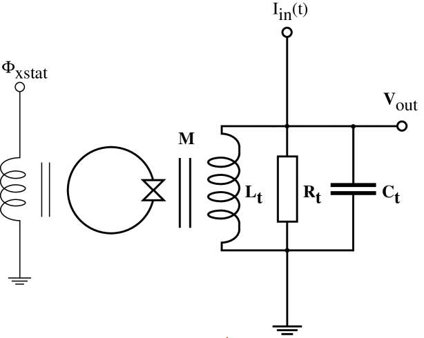
Figure 1: Schematic of the inductively coupled SQUID ring-tank circuit system.

In the most commonly used experimental scheme the dynamical behaviour of the ring is followed in the time domain through the so-termed SQUID magnetometer characteristics. In these, the rf voltage $\left(V_{\text{out}}\right)$ developed across the tank circuit is plotted as a function of the rf current $\left(I_{\text{in}}\right)$ used to excite it, where $I_{\text{in}}$ is linearly amplitude modulated in time (figure 1). This current generates an rf flux (peak amplitude $\varphi$) in the tank circuit inductor (coil), a fraction of which ($\mu=M/L_{\text{t}}$ for a coil-ring mutual inductance of $M$) then couples to the SQUID ring. The supercurrent response in the ring then back-reacts on the tank circuit, and so on. Any additional static or quasi-static magnetic flux $\left(\Phi_{\text{xstat}}\right)$ that is required is usually supplied via a second coil coupled to the SQUID ring, again as depicted in figure 1. For small $\beta$-values (i.e. from $<1$ to a few) the $V_{\text{out}}$ versus $I_{\text{in}}$ dynamics contain as their main element a set of voltage features repeated periodically in $I_{\text{in}}$ at intervals $\varpropto\Phi_{\text{o}}/\Lambda$. The precise form of the SQUID magnetometer characteristics depends both on the type of rf detection employed (e.g. phase sensitive or diode) and the value of $\Phi_{\text{xstat}}$.

The non-linear screening current response can also be made manifest in the frequency domain. This can be accomplished at a fixed level of (peak amplitude) rf flux $\mu\varphi$ at the SQUID ring, without the need for amplitude modulation. For example, in the inductive regime, with $\beta$ very close to one from below, we have demonstrated that, at sufficiently large values of $\mu\varphi$, fold bifurcations develop in the resonance lineshape of a SQUID ring-tank circuit system. Indeed, using a bidirectional sweep (up and down in frequency), and at certain values of $\mu\varphi$ and $\Phi_{\text{xstat}}$, the system can even display opposed (hammerhead) fold bifurcations in this lineshape, one on each side of the resonance 7 . Opposed bifurcations are not only most unusual but, to our knowledge, the possibility of their existence is scarcely mentioned in the literature on non-linear dynamics 8 . In the case of the inductive SQUID ring, with $\beta$ very close to one, we have found that these bifurcations are always well separated in frequency. However, in this work we will show that in the weakly hysteretic regime of SQUID behaviour $\left(\beta\approx few\right)$ this separation can become extremely, perhaps vanishingly, small. Throughout this work we shall term this a pinch resonance.

The one sided (above or below resonance) weak fold bifurcation 9 is taken as the text book example of the onset of non-linear behaviour in a strongly driven oscillator. The development of opposed fold bifurcations (on both sides of the resonance) in any non-linear system is another matter altogether. As far as we are aware, opposed fold bifurcations had not be seen experimentally prior to our report of hammerhead resonances in the frequency domain of coupled inductive SQUID ring-tank circuit systems 7 , and only once in the theoretical literature 8 . In itself, we consider that this constitutes a significant contribution to the body of knowledge concerning non-linear dynamical systems. That the cosine non-linearity of the SQUID ring can also generate, in part of its parameter space, something as exotic a a pinch resonance is simply remarkable, particularly since such resonances appear as solutions to the established equations of motion for the ring-tank system in the weakly hysteretic regime. What this result, and others, point to is that the non-linear dynamics of SQUID rings coupled to other, linear, circuits is likely to prove very rich indeed 10 , the more so since the parameter space that has so far been explored is still very limited. As such, these coupled systems are likely to continue to be a focus of attention by the non-linear community, both in theory and experiment.

With the SQUID ring treated, as in this paper, quasi-classically, there would appear to be many potential applications of its intrinsic non-linear nature when coupled to external circuits, for example, in logic and memory (single 11 or multi-level 12 ), stochastic resonance 13 and in safe communication systems based on chaotic transmission/reception 14 . However, in the last few years there has been a burgeoning interest in exploring the properties of SQUID rings in the quantum regime for use in quantum technologies, particularly for the purposes of quantum computing and quantum encryption 15 ; 16 ; 17 ; 18 . This interest has been boosted by recent experimental work on quantum superposition of states in weak link circuits 19 ; 20 ; 21 ; 22 and very strongly in the last year by reports in the literature of experimental investigations of superposition states in SQUID rings 23 ; 24 . Quantum technologies will, of necessity, involve time dependent superpositions for their operation. Where quantum circuits such as SQUID rings are involved, this means the interaction with external electromagnetic (em) fields or oscillator circuit modes. Correspondingly, the effect of applied em fields (classical or quantum) of high enough frequency and amplitude is to generate quantum transition regions where energy is exchanged between the ring energy levels. Given the cosine term in the SQUID ring Hamiltonian 6 , these energy exchanges in general involve (non-perurbatively) coherent multiphoton absorption or emission processes 25 ; 26 . These exchange regions extend over very small ranges in the static magnetic flux $\Phi_{\text{xstat}}$ applied to the ring (typically over $10^{-3}$ to $10^{-4}\Phi_{\text{o}}$), comparable to the width of the anticrossing regions reported in the recent experiments on superposition of states in SQUID rings 23 ; 24 . Such narrow flux widths imply the concomitant existence of extremely strong non-linearities in the screening supercurrents flowing in the ring. In general these current non-linearities generate non-linear dynamical behaviour in external (classical) circuits used to probe the superposition state of the ring. As we have emphasized in previous publications 27 ; 28 ; 29 , following these non-linear dynamics is one way of extracting information concerning the quantum state of a SQUID ring, or any other quantum circuit based of weak link devices. From our perspective, therefore, it is of clear importance to the future development of quantum technologies based on SQUID rings and related devices that these non-linear dynamics be studied in great detail. Given the results presented in this paper, the non-linear dynamics of coupled SQUID ring-probe circuit systems can display rich and yet unanticipated behaviour. With these rings operating in the quantum regime this is even more likely to be the case.

II Experimental Pinch Resonances

Although sometimes unappreciated, probing the non-linear dynamical behaviour of SQUID ring-tank circuit systems makes strong demands on the high frequency electronics used. In order to open up new non-linear phenomena in these systems we required rf electronics which combined ultra low noise performance, large dynamic range and high slew rate capability. In practice we achieved this by using a liquid helium cooled (4.2 Kelvin), GaAsFET-based, rf amplifier (noise temperature $\lessapprox$ 10 Kelvin, gain close to 20dB) followed by a state of the art, low noise, room temperature rf receiver. With these electronics we could choose diode or phase sensitive detection of $V_{\text{out}}$. Since phase sensitive detection generally provides better signal to noise, this was always our chosen mode of operation for acquiring SQUID magnetometer characteristics.

In the work reported in this paper the SQUID rings used were of the Zimmerman two hole type 30 . These were fabricated in niobium with a niobium weak link of the point contact kind. This weak link was formed by mechanical adjustment between a point and a post screw, the latter having a plane machined end face which had been preoxidized prior to its insertion in the SQUID block. The weak link was made in situ at 4.2 Kelvin via a room temperature adjustment mechanism. As we have shown in previous publications 7 , the control we can exert using this mechanism is very good, sufficient in fact to make reproducible point contact SQUID rings with any desired $\beta$ value from inductive 7 to highly hysteretic 12 .

In figure 2

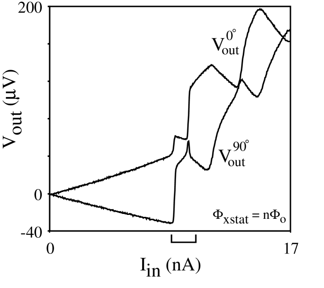
Figure 2: Experimental equal amplitude (phase sensitive detected and $90^{\text{o}}$ apart in phase) rf SQUID magnetometer characteristics ($V_{out}$ versus $I_{\text{in}}$) of a weakly hysteretic $\left(\beta=2.26\right)$ niobium point contact SQUID ring at a static flux bias of $\Phi_{\text{xstat }}=n\Phi_{\text{o}}$. Here, $\Lambda=6\times 10^{-10}H$, $\omega_{\text{in }}/2\pi=20.122MHz$, $L_{\text{t}}=6.3\times 10^{-8}H$, $Q=1058$, $K^{2}=4\times 10^{-3}$ and T = 4.2 Kelvin.

we show what we term the equal amplitude magnetometer characteristics for a weakly hysteretic ($\beta$ close to $2$) niobium point contact SQUID ring coupled to an rf tank circuit. In these characteristics, taken at 4.2 Kelvin with a static bias flux of $n\Phi_{\text{o}}$, the frequency of the drive current was set to the coupled SQUID block-tank circuit resonant frequency before a weak link contact was made $\left(\text{i.e. }\omega_{\text{in}}/2\pi\right)$ and the voltage components ($V_{\text{out}}^{0^{\text{o}}}$ and $V_{\text{out }}^{90^{\text{o}}}$) were maintained exactly $90^{\text{o}}$ out of phase. However, their relative phases with respect to $I_{\text{in }}$ were rotated electronically until the average slopes of the two characteristics are essentially equal. This approach was adopted for convenience - it presented the periodic features in $I_{\text{in}}$ of the orthogonal phase components of $V_{\text{out}}$ at essentially the same amplitude. Here, the (measured) ring inductance $\Lambda=6\times 10^{-10}H$, the measured ring-tank circuit coupling coefficient $K^{2}\left(=\frac{M^{2}}{\Lambda L_{\text{t}}}\right)=0.004$, $L_{\text{t}}=6.3\times 10^{-8}H$, $Q$ $=1058$ and the drive (excitation) frequency for $I_{\text{in}}$, $\omega_{\text{in}}/2\pi=20.122MHz$. It is apparent from figure 2 that even in this weakly hysteretic regime the observed SQUID magnetometer characteristics are highly non-linear and contain a wealth of detail.

Some of the time domain information of figure 2 can be recast in a quite dramatic form in the frequency domain. To extract this experimentally requires the use of a high performance spectrum analyzer with a tracking generator output 7 . This output provides a voltage signal of constant peak to peak amplitude over the frequency range of interest. Feeding this through a series high impedance generates an rf current in the tank circuit which, in turn, creates an rf flux ( peak amplitude $\mu\varphi$) at the SQUID ring. As with our previous work on SQUID ring-tank circuit dynamics in the inductive regime 5 ; 7 , the details of this behaviour depend crucially on the value of the static bias flux $\Phi_{\text{xstat}}$.

In figure 3

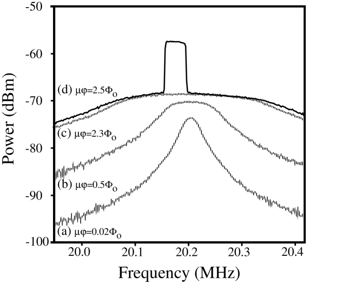
Figure 3: (a) to (d) T = 4.2 Kelvin, $\Phi_{\text{stat}}=\left(n+1/2\right)\Phi_{\text{o}}$ plots of the unidirectional frequency sweeps (from low to high) for the weakly hysteretic $\left(\beta=2.26\right)$ ring-tank circuit system of figure 2 for different peak rf flux amplitudes at the SQUID ring (i.e. $\mu\varphi=0.02,0.5,2.3$ and $2.5\Phi_{\text{o}}$ ) showing the punch through at higher amplitude (e.g. $\mu\varphi\gtrapprox 2\Phi_{\text{o}}$).

we show four frequency responses for unidirectional sweeps, from low to high frequency, for the SQUID ring-tank circuit system of figure 2 (at T = 4.2 Kelvin). The data were taken at rf flux amplitudes $\mu\varphi$ ranging from $0.02$ to $2.5\Phi_{\text{o}}$, with $\Phi_{\text{xstat}}=\left(n+1/2\right)\Phi_{\text{o}}$. These frequency responses were recorded using a high performance, but conventional, commercial spectrum analyzer (a Rohde and Schwarz FSAS system) which could only scan in this unidirectionally manner. What is clear from figure 3 is that as $\mu\varphi$ becomes a significant fraction of a flux quantum the lineshape of the frequency response curves changes dramatically. In particular, for $\mu\varphi\gtrapprox 2\Phi_{\text{o}}$ there is a punch through effect which leads to the creation of fold bifurcation cuts. If we refer back to figure 2, this value of peak rf flux $\mu\varphi$ equates to a drive current corresponding to the feature shown bracketed in figure 2, but for the case of static bias flux $\Phi_{\text{xstat}}=\left(n+1/2\right)\Phi_{\text{o}}$. The significance of this was revealed when bidirectional frequency sweeps (from low to high and then high to low) were taken using a spectrum analyzer of our own design. This spectrum analyzer is shown in block form in figure 4

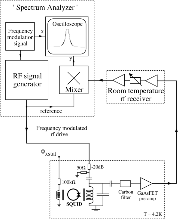
Figure 4: Block diagram of the spectrum analyzer used to record the bidirectional frequency response curves of figure 5.

. As an illustration of its utility, we show in figure 5

Figure 5: Expanded, bidirectional, frequency sweeps (low to high and then high to low) for the response (d) in the data of figure 3, again with $\mu\varphi=2.5\Phi_{\text{o}}$ and T = 4.2 Kelvin. This value of peak $\mu\varphi$ equates to a drive current, at static bias flux $\Phi_{\text{xstat }}=\left(n+1/2\right)\Phi_{\text{o}}$, corresponding to the feature shown bracketed in figure 2.

the result of this bidirectional sweep for the curve (d) of figure 3 ($\mu\varphi=2.5\Phi_{\text{o}}$), again at $\Phi_{\text{xstat}}=\left(n+1/2\right)\Phi_{\text{o}}$. As can be seen in figure 5, there are four fold bifurcation cuts, one each at the lowest and highest frequency excursions in the response, and two inner cuts, one on the sweep up and the other on the sweep down. Within the experimental resolution, as reflected in the data points, these inner cuts appear to overlay exactly. To our knowledge, this has not been observed before. For this bidirectional response it seems reasonable to adopt the description pinch resonance.

The frequency response curve of figure 5 and those plotted in figure 3 as a function of coupled rf amplitude, are perfectly typical of the low $\beta$ value ($\approx$ few) hysteretic SQUID ring-tank circuit systems that we have studied. To aid in interpretation we have provided in figure 6

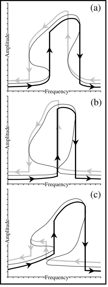
Figure 6: A schematic of three different bidirectional frequency response curves: (a) where the inner pair of opposed fold bifurcation cuts are well separated in frequency (b) where these cuts superimpose in frequency (a pinch resonance) and (c) where the fold bifurcations have moved beyond one another.

a schematic of three different bidirectional frequency response curves: (a) where the inner pair of opposed fold bifurcation cuts are well separated in frequency (b) where these cuts superimpose in frequency (i.e. in our terminology, a pinch resonance) and (c) where the fold bifurcations have moved beyond one another. It seems clear that the data of figure 5 correspond to the bidirectional response of figure 6(b) since this response can obviously be differentiated from those of figures 6(a) and 6(c). It is interesting to note that the existence of any one of the bidirectional response curves shown schematically in figure 6 could not be revealed using standard commercial spectrum analyzers since these always sweep the frequency unidirectionally, i.e. from low to high. For completeness, we show in figure 7

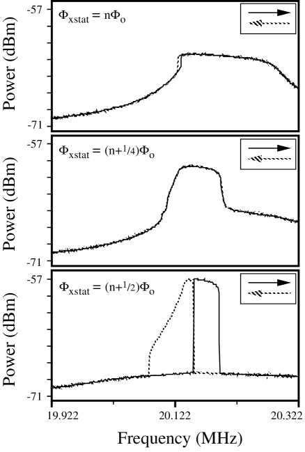
Figure 7: Experimental bidirectional frequency response curves for the SQUID ring-tank circuit system of figures 3(d) and 5 (T = 4.2Kelvin, $\mu\varphi=2.5\Phi_{\text{o}}$) at three values of static bias flux at the ring $\Phi_{\text{xstat}}=n\Phi_{\text{o}}$, $\left(n+1/4\right)\Phi_{\text{o}}$ and $\left(n+1/2\right)\Phi_{\text{o}}$.

the bidirectional frequency responses (with both up and down sweeps) for the ring-tank circuit system of figures 3(d) and 5 $\left(\text{T = 4.2 Kelvin},\mu\varphi=2.5\Phi_{\text{o}}\right)$ at the static bias flux values $\Phi_{\text{xstat}}=n\Phi_{\text{o}}$, $\left(n+1/4\right)\Phi_{\text{o}}$ and $\left(n+1/2\right)\Phi_{\text{o}}$. As is apparent, the pinch resonance can only be seen in one of these responses, i.e. at $\Phi_{\text{xstat}}=\left(n+1/2\right)\Phi_{\text{o}}$.

III Theoretical Model

III.1 RSJ+C description

In the standard dynamical description of a SQUID ring it is customary to invoke the well known (quasi-classical) resistively shunted junction plus capacitance (RSJ+C) model 4 of the weak link in the ring. Here, a pair (Josephson) current channel is in parallel with an effective weak link capacitance $C$ and a normal current channel of resistance $R$. For an applied current $I>I_{\text{c}}$, the normal channel opens up with a value of $R$ which is characteristic of the particular weak link in the ring. In this (and other) models the SQUID ring moves in the space of total included magnetic flux $\Phi=\Phi_{\text{x}}+\Lambda I_{\text{s}}$ with an effective mass given by the weak link capacitance $\left(C\right)$. Within the RSJ+C model it is always assumed that the SQUID ring can be treated as a quasi-classical object, such that $C$ is relatively large, typically $\approx 10^{-13}$ to $10^{-14}F$.

In the RSJ+C description the SQUID ring and tank circuit constitute a system of coupled oscillators with equations of motion which can be written in the form

tank circuit

$$C_{\text{t}}\ddot{\varphi}+\frac{\dot{\varphi}}{R_{\text{t}}}+\frac{\varphi}{L_{\text{t}}}=I_{\text{in}}+\frac{K^{2}\Phi}{M\left(1-K^{2}\right)}$$ (1)

where $R_{\text{t}}$ is the tank circuit resistance on parallel resonance of the coupled system and $I_{\text{in}}$ is the drive current (figure 1), which may contain both coherent and noise contributions.

SQUID ring

$$C\ddot{\Phi}+\frac{\dot{\Phi}}{R}+\frac{\Phi}{\Lambda\left(1-K^{2}\right)}+I_{\text{c}}\sin\left(\frac{2\pi\Phi}{\Phi_{\text{o}}}\right)=\frac{K^{2}\varphi}{M\left(1-K^{2}\right)}$$ (2)

where $I=I_{\text{c}}\sin\left(\frac{2\pi\Phi}{\Phi_{\text{o}}}\right)$ is the phase dependent Josephson current for the weak link in the ring.

Until recently little effort appears to have been directed to solving the coupled equations in their full non-linear form, understandably given the level of computational power required to deal with them. Instead it has often been assumed that it is sufficiently accurate to linearize the SQUID ring equation of motion. This is equivalent to invoking the adiabatic condition that the ring stays at, or very close to, the minimum in its potential

$$U\left(\Phi,\Phi_{\text{x}}\right)=\frac{\left(\Phi-\Phi_{\text{x}}\right)^{2}}{2\Lambda}-\frac{I_{\text{c}}\Phi_{\text{o}}}{2\pi}\cos\left(\frac{2\pi\Phi}{\Phi_{\text{o}}}\right)$$ (3)

as this varies with time. The SQUID equation (2) then reduces to

$$I_{\text{c}}\sin\left(\frac{2\pi\Phi}{\Phi_{\text{o}}}\right)+\frac{\Phi}{\Lambda\left(1-K^{2}\right)}=\frac{K^{2}\varphi}{M\left(1-K^{2}\right)}$$ (4)

However, as we have shown in recent work 12 , this approximation should be treated with great care, particularly in the hysteretic regime of behaviour. In order to avoid this problem we have chosen to solve the full coupled equations of motion [(1) and (2)] for the system using values of $C$ and $R$ considered typical of a weakly hysteretic SQUID ring. We shall demonstrate that pinch resonances, such as we have presented in figure 5, and which match with the experimentally determined circuit parameters, show up as solutions of these equations.

III.1.1 Pinch resonances

With a knowledge of the system parameters, and an estimate of $I_{\text{c}}$ , we can solve the coupled equations of motion (1) and (2) numerically to find the value, at a given $\Phi_{\text{xstat}}$, of the rf tank circuit voltage $\dot{\varphi}$ as a function of the frequency of the fixed amplitude sinusoidal drive current $I_{\text{in }}$. This voltage response can then be used to compute the bidirectional frequency responses of the ring-tank circuit system. To do this we considered an interval $\left[\omega_{\text{min}}/2\pi\text{ to }\omega_{\text{max}}/2\pi\right]$ in the drive frequency which contained the (peak amplitude) resonant frequency of the system. This interval was divided into $N$ bins which gave us a resolution of $\delta\omega=\left(\omega_{\text{ max}}-\omega_{\text{min}}\right)/N$ in the frequency domain. We then drove the tank circuit at $\omega_{\text{in}}$ (for $I_{\text{in}}$)$=\omega_{\text{min}}+n\delta\omega$ for $n=0,1,.....,N$ increments in frequency (this being done without changing the initial conditions of the system), thus obtaining the power in the tank circuit at each of these frequencies via 5 ; 7

$$P\left(\omega_{\text{in}}\right)=\frac{2}{\left(2\pi m/\omega_{\text{in}}\right)}\left|\int_{\text{o}}^{2\pi m/\omega_{\text{in}}}\dot{\varphi}\exp\left(i\omega_{\text{in}}t\right)dt\right|^{2}$$ (5)

for a given integer $m$. We note that $m$ is taken so that the power is integrated over a few $Q$ cycles of the tank circuit oscillation to reduce the effects of transients. In the situation where the non-linearities in the coupled ring-tank circuit system are strong, and where, typically, the rf drive amplitudes are large, we have already shown 5 ; 7 that fold bifurcation regions (i.e. regions where more than one stable solution exists) can develop in the resonance curves of the system.

To make a comparison with the experimental data of figure 5 we estimated the value of the $\beta$-parameter from the $0^{\text{o}}$ SQUID magnetometer characteristic of figure 2 using the ratio (on the current axis $I_{\text{in}}$) of the initial riser to the interval between the periodic features in this characteristic. This yielded a $\beta$ value of $2.26$, which, for a ring inductance of $6\times 10^{-10}H$, set $I_{\text{c}}=1.23\mu A$. In a recent publication we described a quantum electrodynamic model 31 of a SQUID ring which has allowed us to derive an expression for the effective ring capacitance $\left(C\right)$, knowing the superconducting material from which it is constructed and the value of the weak link critical current. With niobium as the material, and $I_{\text{c}}\cong 1$ to a few $\mu A$, this yields $C\lessapprox 10^{-14}F$. An alternative model 32 , using a different approach, gives rise to similar size capacitances. From the literature 32 ; 33 , a corresponding effective dissipative resistance in the ring $\approx 100\Omega$ appears perfectly reasonable, setting a ring $CR$ time constant of $10^{-12}$secs.

The theoretical bidirectional frequency response curves corresponding to the experimental data (and circuit parameters) of figure 5 are shown in

figure 8

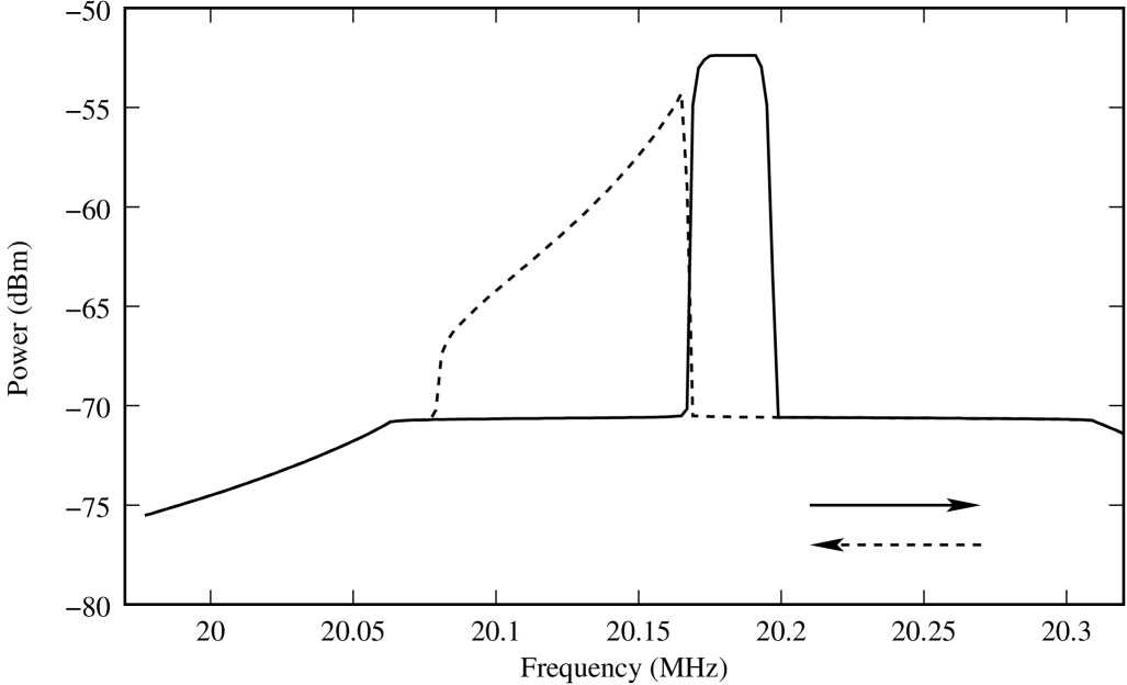
Figure 8: Computed (RSJ+C model) bidirectional, frequency response curves (low to high and then high to low) using the ring and tank circuit parameters of figures 2 and 5 with $I_{\text{c}}=1.23\mu A$, $C=10^{-14}F$ and $R=100\Omega$ ($CR=10^{-12}\sec$).

, with $I_{\text{c}}$ and $CR$ taken to be $1.23\mu A$ and $10^{-12}$ secs, respectively. These were computed, sweeping forwards and backwards across the defined frequency window, using a 4${}^{\text{th}}$ order Runge-Kutta-Merson routine with adaptive step size error control. The SQUID ring-tank circuit coupling $\left(K^{2}\right)$ and $Q$ parameters were set as for figures 3(d) and 5 together with $\mu\varphi=2.5\Phi_{\text{o}}$ and $\Phi_{\text{xstat}}=\left(n+1/2\right)\Phi_{\text{o}}$. From numerous computations we have found that the shape of the bidirectional response in this RSJ+C approach is determined principally by the $CR$ product and is only weakly dependent on the particular values of $C$ and $R$ chosen, at least in the ranges $10^{-12}$ to $10^{-14}F$ and $1$ to $100\Omega$. With the circuit parameters detailed above, we found that the best fit to figure 5 (the pinch off resonance) is made with $CR=10^{-12}$ secs. As for the experimental data displayed in figure 5, the theoretical inner fold bifurcation cuts superimpose very well, at least to the limits of our computational accuracy. This is reflected in the computed data points in the region of these inner cuts.

Clearly, the correspondence between the theoretically calculated response curves of figure 8 and the experimental bidirectional responses of figure 5 is good, both in frequency range and lineshape. For example, at $\Phi_{\text{xstat}}=\left(n+1/2\right)\Phi_{\text{o}}$ the experimental and theoretical responses appear to meet exactly at one point in the frequency domain. However, we must caution that due to the numerical nature of the calculation it is not possible theoretically to prove that this single frequency meeting point is exact. Nevertheless, by trying different amplitudes for $I_{\text{in}}$ we have found that we can narrow the separation between the solutions down to an arbitrarily small level. This reflects the situation found experimentally. We note that we have been unable to generate this theoretical fit to our experimental bidirectional reponse curves using the linearized SQUID equation (4).

With regard to the alternative frequency response curves of figure 6, and the experimental data of figures 5 and 7, we note that it may be appropriate to treat this weakly hysteretic SQUID ring-tank circuit system as an extremely sensitive finite state machine 34 . If so, we may be able to compare the transition state diagram for the different cycles shown in figure 6 [(a), (b) and (c)]. As an example, we may ask whether it is possible in the pinch resonance (b) to go between the lower left and lower right branches without jumping up to the loop. This could happen occasionally but still be beyond the sensitivity limits of our present experimental apparatus. If it does occur there will be a sharp transition between the full pinch loop resonance [fine black line in figure 6(b)] and the resonance displaying sets of bifurcation cuts., i.e. in the one case the resonance loop is not accessed, in the other (the latter) it is. In principle, the two processes could be distinguished since the pathways around the loop involve very much larger voltages than the crossing between the lower branches of the resonance. Such contrasting processes would, of course, be of scientific interest but could also have potential in device applications.

IV Conclusions

In this paper we have shown that a single weak link SQUID ring, weakly hysteretic and coupled to a simple parallel resonance tank circuit, can display quite remarkable, and previously unexpected, non-linear behaviour in the frequency domain. Thus, we have demonstrated that this system exhibits opposed fold bifurcation cuts in its bidirectional frequency response curves which, at specific values of rf and static bias flux, and within our experimental resolution, superimpose exactly. Since single fold bifurcations in the upper or lower branches of a strongly driven resonant system are usually taken as one of the standard examples of the onset of non-linear dynamics 9 , the onset of opposed fold bifurcations is of special note. That this can result, as a limiting case, in the creation of a pinch resonance would appear to be exceptional and, in our opininion, of very considerable interest to the non-linear community. Nevertheless, as we have also shown, such pinch off resonances can be modelled well within the full, non-linear RSJ+C description of the ring-tank circuit system. Together with other recent published work 12 , these results would appear to suggest that there is still a great deal to be explored in the non-linear dynamics of SQUID ring-resonator systems in the quasi-classical regime. It is also apparent that the new non-linear dynamical results obtained in this regime point to future research needed to implement quantum technologies based on SQUID rings (and related weak link devices) interacting with classical probe circuits 5 ; 7 ; 30 . From both perspectives it is clear that the SQUID ring which, through the cosine term in its Hamiltonian, is non-linear to all orders, is set to continue to reveal new and interesting non-linear phenomena of importance in the field of non-linear dynamics and in the general area of the quantum-classical interface as related to the measurement problem in quantum mechanics. It is also apparent that in both the classical and quantum regimes the non-linear dynamics generated in coupled circuit systems involving SQUID rings could form the basis for new electronic technologies.

V Acknowledgements

We would like to thank the Engineering and Physical Sciences Research Council for its generous funding of this research.

References

- (1) W.C.Schieve, A.R.Bulsara, and E.W.Jacobs, Phys. Rev. A 37, 3541 (1988).
- (2) A.R.Bulsara, J. Appl. Phys. 60, 2462 (1986).
- (3) M.P.Soerensen, M.Barchelli, P.L.Christiansen, and A.R.Bishop, Phys. Lett. 109A, 347 (1985).
- (4) K.K.Likharev, “Dynamics of Josephson Junctions and Circuits” (Gordon and Breach, Sidney, 1986).
- (5) T.D.Clark, J.F.Ralph, R.J.Prance, H.Prance, J.Diggins, and R.Whiteman, Phys. Rev. E 57, 4035 (1998).
- (6) T.P.Spiller, T.D.Clark, R.J.Prance and A.Widom, Prog. in Low Temp. Phys., Vol. XIII, edited by D.F.Brewer (North Holland, Amsterdam, 1992), p.219.
- (7) R.Whiteman, J.Diggins, V.Schöllmann, T.D.Clark, R.J.Prance, H.Prance, and J.F.Ralph, Phys. Lett. A 234, 205 (1997).
- (8) A.H.Nayfeh, S.A.Nayfeh, and M.Pakdemirli, in “Non-linear Dynamics and Stochastic Mechanics”, edited by W.Kleinmann and N.Sri Namachchivaya (CRC, Boca Raton, FL, 1995), p. 190.
- (9) L.D.Landau and E.M.Lifshitz, “Mechanics - Course in Theoretical Physics, Vol. 1 ” (Pergamon Press, Oxford, 1987), p.89.
- (10) See, for discussions of bifurcations, etc. in non-linear systems, D.Zwillinger, “Handbook of Differential Equations” (Academic Press, Boston, 1992), p.16 and S.H.Strogatz, “Non-linear Dynamics and Chaos” (Perseus Books, Reading, Massachusetts, 1994), p.44.
- (11) See V.P.Koshelets, K.K.Likharev and V.V. Migulin, IEEE T MAGN 23 : (2) 755 (Mar. 1987); H.Miyake, N. Fukaya and Y. Okabe, IEEE T MAGN 21: (2) 578 (1985).
- (12) R.J.Prance, R.Whiteman, T.D.Clark, H.Prance, V.Schöllmann, J.F.Ralph, S. Al-Khawaja, and M. Everitt, Phys. Rev. Letts. 82, 5401 (1999).
- (13) See, for example A.R.Bulsara and L.Gammaitoni, Phys. Today 49: (3) 39 (1996); L.Gammaitoni, P.Hänggi, P.Jung and F.Marchesoni, Rev. Mod. Phys. 70, 1 (1998)
- (14) See, for example, M.Hasler, International Journal of Bifurcation and Chaos 8, 647 (1998).
- (15) See, for example,“Introduction to Quantum Computation and Information”, eds. H.K. Lo, S. Popescu and T.P. Spiller (World Scientific, New Jersey, 1998).
- (16) T.P. Orlando, J.E. Mooij, L. Tian, C.H. van der Wal, L.S. Levitov, S. Lloyd and J.J. Mazo, Phys. Rev. B. 60, 15398 (1999).
- (17) Y. Makhlin, G. Schön and A. Shnirman, Nature 398, 305 (1999).
- (18) D. Averin Nature 398, 748 (1999).
- (19) R. Rouse, S. Han, J.E. Lukens, Phys. Rev. Lett. 75, 1614 (1995).
- (20) P.Silvestrini, B.B. Ruggierio, C. Granata, E. Esposito, Phys. Lett. A 267, 45 (2000).
- (21) Y. Nakamura, C.D. Chen, J.S. Tsai, Phys. Rev. Lett 79, 2328 (1997).
- (22) Y. Nakamura, Y.A. Pashkin, J.S. Tsai, Nature 398, 786 (1999).
- (23) J.R. Friedman, V. Patel, W. Chen, S.K. Tolpygo, J.E. Lukens, Nature 406, 43 (2000).
- (24) C.H. van der Wal, A.C.J. ter Haar, F.K. Wilhem, R.N. Schouten, C.J.P.M. Harmans, T.P. Orlando, S. Lloyd, J.E. Mooij, Science 290, 773 (2000).
- (25) T.D. Clark, J. Diggins, J.F. Ralph, M.J. Everitt, R.J. Prance, H. Prance, R. Whiteman, A. Widom, and Y.N. Srivastava, Annals Phys. 268 , 1 (1998).
- (26) M.J.Everitt, P.Stiffell, T.D.Clark, A.Vourdas, J.F.Ralph, H.Prance and R.J.Prance, “A Fully Quantum Mechanical Model of a SQUID Ring Coupled to an Electromagnetic Field”, to be published in Phys. Rev. B, April 1, 2001.
- (27) R.Whiteman, V.Schöllmann, M.Everitt, T.D.Clark, R.J.Prance, H.Prance, J.Diggins, G.Buckling and J.F.Ralph, J.Phys.: Condens. Matter 10, 9951 (1998).
- (28) T.D.Clark, J.F.Ralph, R.J.Prance, H.Prance, J.Diggins and R.Whiteman, Phys. Rev. E 57, 4035 (1998).
- (29) R.Whiteman, T.D.Clark, R.J.Prance, H.Prance, H.Prance, V.Schöllmann, J.F.Ralph, M.Everitt and J.Diggins, Journal of Mod. Optics 45, 1175 (1998).
- (30) J.E.Zimmerman, P.Thiene, and J.T.Harding, J. Appl. Phys. 41, 1572 (1970).
- (31) J.F.Ralph, T.D.Clark, J.Diggins, R.J.Prance, H.Prance, and A.Widom, J.Phys. Condens. Matter 9, 8275 (1997).
- (32) K.Gloss, and F.Anders, J. Low Temp. Phys. 116, 21 (1999).
- (33) J.E.Zimmerman, Proc. 1972 Applied Superconductivity Conference, Annapolis, 544-561 (IEEE Publications, New York, 1972).
- (34) R.P.Feynman, “Feynman Lectures on Computation”, eds. A.J.G.Hey and R.W.Allen (Penguin, London, 1999), p.55.