Modelling of Quantum Electromechanical Systems

Modelling of Quantum Electromechanical Systems

ANTTI-PEKKA JAUHO, TOMÁŠ NOVOTNÝ, ANDREA DONARINI, and CHRISTIAN FLINDT

MIC – Department of Micro and Nanotechnology, Technical University of Denmark, Bldg. 345East
DK-2800 Lyngby, Denmark

antti@mic.dtu.dk

Abstract. We discuss methods for numerically solving the generalized Master equation GME which governs the time-evolution of the reduced density matrix $\hat{\rho}$ of a mechanically movable mesoscopic device in a dissipative environment. As a specific example, we consider the quantum shuttle – a generic quantum nanoelectromechanical system (NEMS). When expressed in the oscillator basis, the static limit of the GME becomes a large linear non-sparse matrix problem (characteristic size larger than $10^{4}\times 10^{4}$) which however, as we show, can be treated using the Arnoldi iteration scheme. The numerical results are interpreted with the help of Wigner functions, and we compute the current and the noise in a few representative cases.

Keywords: SET, Coulomb blockade, Nanoelectromechanics, Noise

1. Introduction

Microelectromechanical systems (MEMS) are approaching the nanoscale, which ultimately implies that the mechanical motion needs to be treated quantum mechanically. An example is the experiment by Park et al. [1], where the break junction technique was used to create a single-electron transistor with a C₆₀-molecule as the active part. The measured IV-curves display features that can be related to the mechanical vibrations of the molecule. Already earlier it was suggested theoretically [2] that a nanoscopic movable metallic grain, when operated in the Coulomb blockade regime, can move charges one-by-one between source and drain contacts. This orderly transport was coined the shuttle regime. In recent years our group has developed theoretical methods to analyze the shuttle transition in the quantum regime [3, 4, 5, 6], focusing not only on the IV-curve, but also considering noise and full counting statistics, which are important diagnostic tools in unravelling the microscopic transport mechanisms. In this paper we present examples of our numerical results and discuss pertinent computational issues.

2. The generalized Master Equation (GME)

The Hamiltonian for the system includes terms describing (i) the electronic part of the movable quantum dot (QD for short), (ii) its mechanical motion (which is quantized), (iii) the position dependent coupling of the QD and the leads, (iv) the leads (treated as noninteracting fermions), and (v) coupling to environment, which damps the mechanical motion [3, 4, 5, 6]. Using methods familiar from quantum optics, we integrate out the environmental degrees of freedom (the lead electrons, and a generic heat bath) to obtain a generalized Master equation for the “system” (= QD + quantized oscillator) density operator:

$$\dot{\rho}(t)={\mathcal{L}}\rho(t)=(\mathcal{L}_{\rm coh}+\mathcal{L}_{\rm driv}+\mathcal{L}_{\rm damp})\rho(t).$$ (1)

Here $\mathcal{L}_{\rm coh},\mathcal{L}_{\rm driv}$ and $\mathcal{L}_{\rm damp}$ are superoperators corresponding to the coherent evolution, coupling to leads, and damping of the QD. It is sufficient to consider the diagonal electronic components (i.e., an empty and an occupied QD, respectively), which satisfy [3, 8]

$$\dot{\rho}_{00}(t) = \frac{1}{i\hbar}[H_{\rm osc},\rho_{00}(t)]-\frac{\Gamma_{L}}{2}(e^{-\frac{2x}{\lambda}}\rho_{00}(t)$$

$$+\rho_{00}(t)e^{-\frac{2x}{\lambda}})+\Gamma_{R}e^{\frac{x}{\lambda}}\rho_{11}(t)e^{\frac{x}{\lambda}}$$

$$+\mathcal{L}_{\rm damp}\,\rho_{00}(t)\ ,$$

$$\dot{\rho}_{11}(t) = \frac{1}{i\hbar}[H_{\rm osc}-eEx,\rho_{11}(t)]+\Gamma_{L}e^{-\frac{x}{\lambda}}\rho_{00}(t)e^{-\frac{x}{\lambda}}$$ (2)

$$-\frac{\Gamma_{R}}{2}(e^{\frac{2x}{\lambda}}\rho_{11}(t)+\rho_{11}(t)e^{\frac{2x}{\lambda}})$$

$$+\mathcal{L}_{\rm damp}\,\rho_{11}(t).$$

where

$$\mathcal{L}_{\rm damp}\rho=-\frac{i\gamma}{2\hbar}[x,\{p,\rho\}]-\frac{\gamma m\omega}{\hbar}(\bar{N}+1/2)[x,[x,\rho]]\ .$$

The physical parameters defining the quantum shuttle are thus the couplings to leads $\Gamma_{L/R}$, the oscillator frequency $\omega$, the damping rate of the oscillator $\gamma$, the temperature $T$, and the tunnelling length $\lambda$.

3. The numerical solution

We seek the steady state, $\dot{\rho}_{00}=\dot{\rho}_{11}=0$, i.e., the null vector of the Liouvillean, $\mathcal{L}\rho=0$. Suppose we keep $N$ lowest energy states of the oscillator. Since $\hat{\rho}_{00/11}$ are full matrices in the oscillator basis, they both have $N^{2}$ elements. The matrix representation of the Liouville superoperator has thus $2N^{2}\times 2N^{2}$ elements. (The situation is even more demanding if one considers a shuttle with more than just two electronic states, see [5, 7].) We attempted the solution of these equations with standard Matlab routines, such as the singular value decomposition, by gradually increasing the cut-off $N$. As illustrated in Fig. 3., the Liouville matrices are not sparse. Unfortunately, reliable convergence could not be achieved once $N$ approached few tens, which was quite inadequate for physical reasons, which indicated the necessity of using $N\simeq 100\cdots 200$. Figure 1: The nonzero matrix elements of the Liouville superoperator for a three QD device studied in [7, 5] for three values of the cut-off $N=2,5,10$. $nz$ is the number of non-zero elements. Clearly, more powerful numerical schemes are required. One such method is the Arnoldi iteration [9], which has clear advantages compared to singular value decomposition both in terms of computational speed and memory requirements. First, it is not necessary to store the full Liouvillean matrix, and, second, when one seeks the best approximation to the null vector it is possible to work in spaces which are much smaller than the full Liouville space. The central concept in the Arnoldi scheme is the Krylov space, defined as

$$\mathcal{K}_{j}={\rm span}({\mathbf{x}}_{0},{\mathbf{L}}{\mathbf{x}}_{0},...,{\mathbf{L}}^{j-1}{\mathbf{x}}_{0}),$$ (3)

where $j$ is a small integer. The vector ${\mathbf{x}}_{0}$ is a vectorization of some arbitrary state represented by the two matrices $\hat{\rho}_{00/11}$, i.e. a vector of length $2N^{2}$. Note that the calculation of the vectors ${\mathbf{L}}^{i}{\mathbf{x}}_{0},i=1..(j-1)$ can be done directly from the GME, without storing the full Liouvillean matrix. The next step consists of finding an orthonormal basis in the Krylov space, let us denote this by $\{{\mathbf{q}}_{i}\},i=1,...,j$. The method proceeds now by finding an approximate null vector in the Krylov space, spanned by the vectors $\{{\mathbf{q}}_{i}\}$ thus involving matrices of size $j\times j$. In practice, we have found that $j=20$ is sufficient, which makes the calculations very fast, and no supercomputing is necessary. Once the optimal vector in the Krylov space has been found, we can use the coordinates of this vector to construct the estimate ${\mathbf{x}}_{1}$ (which is a vector of length $2N^{2}$) from which the matrices $\rho_{00/11}$ can be reassembled. If the result is not sufficiently close to the null vector of the Liouvillean, one repeats the procedure by constructing the next Krylov space, now using ${\mathbf{x}}_{1}$ as the seed.

The Arnoldi scheme is iterative in its nature, and one must address the issue of convergence. For example, it is not a priori clear how many iterations are needed, and indeed convergence is not always achieved. This problem is solved by the use of a preconditioner. The basic idea is to find an invertible operator $\mathcal{M}$ in the Liouville space, such that the original problem $\mathcal{L}\rho^{\rm stat}=0$ is cast in the form $\mathcal{M}[\mathcal{L}[\rho^{\rm stat}]]=0$, and that the truncated version of the operator $\mathcal{M}\mathcal{L}$ gives rise to a rapidly converging iteration scheme. The Arnoldi scheme is particularly efficient in finding good approximations to eigenvalues (and corresponding eigenvectors) that are separated from the rest of the spectrum. Thus, in our case, the preconditioner should move the eigenvalues with a non-vanishing real part away from the origin of the complex plane. A good candidate for the preconditioner is to use the Sylvester part [10] of $\mathcal{L}$:

$$\mathcal{L}[\rho]=\mathcal{L}_{\rm Sylv}[\rho]+\mathcal{L}_{\rm rest}[\rho],$$ (4)

where the Sylvester part has the structure

$$\mathcal{L}_{\rm Sylv}[\rho] = {\mathbf{A}}\rho+\rho{\mathbf{A}}^{\dagger}$$

$$= \begin{pmatrix}A_{00}\rho_{00}+\rho_{00}A_{00}^{\dagger}&0\\ 0&A_{11}\rho_{11}+\rho_{11}A_{11}^{\dagger}\end{pmatrix},$$

where the elements $A_{00/11}$ can be gleaned off from the GME. The Sylvester part is rapidly invertible, and we thus chose $\mathcal{M}=\mathcal{L}_{\rm Sylv}^{-1}$. In general, it was essential to use the preconditioner, however we stress that the choice is somewhat subtle and there is no unique algorithm for this. We have encountered special situations where the Sylvester preconditioner did not work satisfactorily, and more work is required in refining the numerics in this case.

Once the static density matrix is solved, the current is readily calculable from

$$I^{\rm stat} = e{\rm Tr}_{\rm osc}\{\Gamma_{R}e^{2x/\lambda}\rho^{\rm stat}_{11}\}$$ (5)

$$= e{\rm Tr}_{\rm osc}\{\Gamma_{L}e^{-2x/\lambda}\rho^{\rm stat}_{00}\}.$$

We have recently shown [4] that also the noise, and even the higher cumulants [6], can be calculated with similar methods. In particular, we find that the Fano factor $F=S(0)/2eI$ (here $S(0)$ is the zero-frequency component of the noise spectrum) can be expressed as

$$F = 1-\frac{2e\Gamma_{R}}{I}\mathrm{Tr_{osc}}\left\{e^{\frac{2x}{\lambda}}\left[\mathcal{Q}\mathcal{L}^{-1}\mathcal{Q}\right.\right.$$ (6)

$$\times\left.\left.\begin{pmatrix}\Gamma_{R}e^{\frac{x}{\lambda}}\rho_{11}^{\rm stat}e^{\frac{x}{\lambda}}\\ 0\end{pmatrix}\right]_{11}\right\}\ .$$

Here $\mathcal{Q}$ is a projection operator that projects away from the stationary state. Very importantly, the pseudoinverse $\mathcal{R}$ of the Liouvillean, defined as $\mathcal{Q}\mathcal{L}^{-1}\mathcal{Q}\equiv\mathcal{R}$ is tractable by similar numerical methods as used in the evaluation of the current (we use the generalized minimum residual method (GMRes) [11]). Before showing results for the current and noise, we discuss an important visualization tool.

4. Wigner functions

We have found that Wigner functions are an excellent interpretative tool for the numerical results obtained for the stationary density matrix. The intuitive picture comes from the well-known results in the classical limit: the Wigner representation (or, equivalently, the phase-space representation) of a regularly moving harmonic oscillator is a circle. On the other hand, irregular motion under the influence of external noise gives rise to a Gaussian probability distribution centered at the origin. Since the QD can be either empty or occupied, it is advantageous to introduce charge resolved Wigner functions ($n=0$ corresponds to an empty dot, while $n=1$ represents the occupied dot), defined as

$$W_{nn}(X,P)=\int_{-\infty}^{\infty}\frac{dy}{2\pi\hbar}\,\bigl{\langle}X-\frac{y}{2}\,|\rho_{nn}^{\rm stat}|X+\frac{y}{2}\bigr{\rangle}\exp\bigl{(}i\frac{Py}{\hbar}\bigr{)}.$$ (7)

An example of the empty dot Wigner function is given in Fig. 4.. The shape is consistent with physical intuition. Consider, for example, positive $x$ and positive $p$ (the shuttle is approaching the drain contact). Then the probability of an empty dot is large, because the extra charge is very likely to leave the shuttle as the drain contact is approached. Analogously, at negative $x$ and positive $p$ the probability of an empty dot is very small, because the dot has been recharged in the vicinity of the left (source) contact, and the charge cannot have left the QD because of the exponentially small coupling to the right (drain) contact. Very interestingly, in Fig. 2 we also see an enhanced probability located at the origin of the phase space. The interpretation is that at these values of parameters there are two co-existing transport regimes: (i) the charge shuttling regime (represented by the ring), and (ii) an incoherent tunnelling regime in which charges tunnel into and out from the QD uncorrelated to its position. Figure 2: The Wigner representation of the empty-dot density matrix in the co-existence regime.

5. Numerical results

Figure 3 shows the computed stationary current as a function of the damping rate. Noteworthy features are: (i) One observes a shuttling transition (or, perhaps more appropriately, a cross-over) from a low value of current (tunnelling regime) to a high value of current (shuttling regime) even in the quantum regime (small $\lambda$); (ii) in the low damping limit the current saturates to a universal value of $1/2\pi$ corresponding to precisely one electron transmitted per cycle.

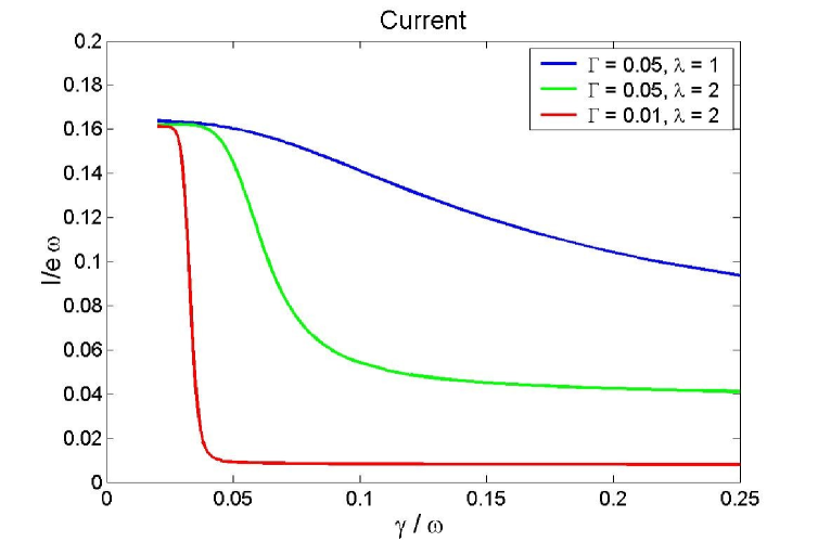
Figure 3: Stationary current as a function of damping rate.

More dramatic effects are observed in the Fano factor, given in Fig. 4. Again, we just list the essential features: (i) For high values of damping, the noise has its Poissonian value ($\simeq 1$); (ii) At low values of damping, the noise is very low (reflecting the orderly nature of the shuttling regime); (iii) At the shuttling cross-over there occurs a large enhancement of the noise.

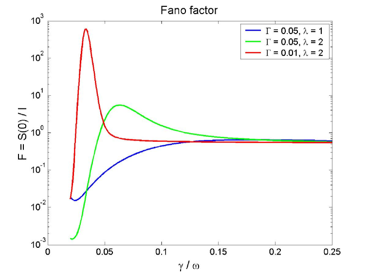
Figure 4: The Fano factor as a function of the damping.

The extraordinarily large values of the Fano factor of the order of 600 can be explained as being a consequence of a slow switching process between two competing current channels (shuttling and tunnelling), and in Ref. [6] we give a detailed analysis of this phenomenon, also supported by semianalytic considerations.

In conclusion, we have presented a numerical technique for solving the generalized Master equation governing a generic quantum nanoelectromechanical device. The obtained numerical results are interpreted with the help of phase space representations. We believe that the methods discussed here are also applicable to many other quantum transport situations, where the matrix representations of the relevant operators are very large, but where only certain extremal eigenvalues are important.

References

- [1] H. Park, J. Park, A. K. L. Lim, E. H. Anderson, A. P. Alivisatos, and P. L. McEuen, Nature 407, 57 (2000).
- [2] L. Y. Gorelik, A. Isacsson, M. V. Voinova, B. Kasemo, R. I. Shekhter, and M. Jonson, Phys. Rev. Lett. 80, 4526 (1998).
- [3] T. Novotný, A. Donarini, and A. P. Jauho, Phys. Rev. Lett. 90, 256801 (2003).
- [4] T. Novotný, A. Donarini, C. Flindt, and A. P. Jauho, Phys. Rev. Lett. 92, 248302 (2004).
- [5] C. Flindt, T. Novotný, and A. P. Jauho, to appear in Phys. Rev. B (2004); cond-mat/0405512.
- [6] C. Flindt, T. Novotný, and A. P. Jauho, to appear in Europhys. Lett. (2004); cond-mat/0410322.
- [7] A. D. Armour and A. MacKinnon, Phys. Rev. B 66, 035333 (2002).
- [8] We show in [3, 4, 5] that the off-diagonal elements decouple from , and are not needed in the evaluation of the stationary limit.
- [9] A good introduction to the Arnoldi scheme can be found in G. H. Golub and C.F. Loan, Matrix Computations, The Johns Hopkins University Press, 3rd Edition (1996).
- [10] Prof. T. Eirola, Private communication.
- [11] C. Flindt, Master’s Thesis, MIC, Technical University of Denmark, URL http://www.mic.dtu.dk/research /TheoreticalNano /publications/ Theses.htm