Oscillations of a Bose-Einstein condensate rotating in a harmonic plus quartic trap

Abstract

We study the normal modes of a two-dimensional rotating Bose-Einstein condensate confined in a quadratic plus quartic trap. Hydrodynamic theory and sum rules are used to derive analytical predictions for the collective frequencies in the limit of high angular velocities, $\Omega$, where the vortex lattice produced by the rotation exhibits an annular structure. We predict a class of excitations with frequency $\sqrt{6}\Omega$ in the rotating frame, irrespective of the mode multipolarity $m$, as well as a class of low energy modes with frequency proportional to $|m|/\Omega$. The predictions are in good agreement with results of numerical simulations based on the 2D Gross-Pitaevskii equation. The same analysis is also carried out at even higher angular velocities, where the system enters the giant vortex regime.

The availability of traps with stronger than harmonic confinement opens up new scenarios in rotating ultracold gases. In principle such traps permit the realization of configurations rotating with arbitrarily high angular velocities, since the confining potential is always stronger than the repulsive centrifugal term. The first experiments in this direction are reported in Ref. ENS .

The stationary configurations of rotating Bose-Einstein condensates in the presence of a harmonic plus quartic trap have already been the subject of several theoretical papers quartic theory ; equilibrium . These calculations predict novel vortex structures reflecting the interplay between the centrifugal and confining forces. In particular, if the angular velocity, $\Omega$, exceeds a critical value, the centrifugal force overcomes the harmonic confinement giving rise to a hole in the center of the condensate. For large angular velocities the radius of the resulting annulus increases linearly with $\Omega$, while the width of the annulus decreases like $1/\Omega$. For such geometries the dynamical behavior of the gas exhibits new features, whose investigation is the main purpose of this work. In particular, along with excitations involving radial deformations of the density, one expects the occurrence of low frequency sound waves propagating around the annulus.

In this work we will calculate the frequencies of the lowest modes by developing an analytical description using hydrodynamic theory and sum rules, as well as carrying out simulations based upon the numerical solution of the Gross-Pitaevskii equation. For simplicity we will restrict our discussion to 2D configurations, valid for fast rotating condensates strongly confined in the axial direction.

The expression for the trapping potential is given by the sum of quadratic and quartic components

$$V_{\text{ext}}=\frac{\hbar\omega_{\perp}}{2}\left(\frac{r^{2}}{d_{\perp}^{2}}+\lambda\,\frac{r^{4}}{d_{\perp}^{4}}\right)\ .$$ (1)

Here $\omega_{\perp}$ is the harmonic oscillator frequency, $d_{\perp}=\sqrt{\hbar/M\omega_{\perp}}$ is the characteristic harmonic oscillator length where $M$ is the atomic mass, $r=\sqrt{x^{2}+y^{2}}$ is the two-dimensional radial coordinate and $\lambda$ is the dimensionless parameter characterizing the strength of the quartic term. In the following, we use dimensionless harmonic oscillator units, where $\omega_{\perp}$ and $d_{\perp}$ are the units of frequency and length respectively.

When the angular velocity $\Omega$ is sufficiently high, a lattice of quantized vortices is formed. If $\lambda>0$, then for $\Omega$ exceeding a critical value, $\Omega_{h}>1$, the equilibrium configuration in the rotating frame corresponds to a vortex lattice with a hole in the center quartic theory ; equilibrium . At even larger angular velocities the system is expected to undergo a transition to a giant vortex where all the vorticity is confined to the center of the annular condensate. In the following we will mainly restrict the discussion to the former regime which is more accessible experimentally, although we briefly discuss the giant vortex at the end.

For a vortex lattice the dynamics can be described by introducing the concept of diffused vorticity within a hydrodynamic picture. This approach has already successfully described the dynamics of rotating configurations in harmonic traps stripes . Such an approximation is valid provided that the Thomas-Fermi condition $\xi\ll d$ is satisfied, where $\xi$ is the healing length and $d$ is the width of the annulus equilibrium . In addition, the healing length should be small compared to the distance $l=1/\sqrt{\Omega}$ between vortices, $\xi\ll l$.

In the rotating frame the linearized rotational hydrodynamic equations take the form

$$\frac{\partial}{\partial t}\,\delta{n}+\bm{\nabla}\cdot({n}_{0}\,\delta\bm{v})\,\ =\,\ 0\ ,$$ (2)

$$\frac{\partial}{\partial t}\,\delta\bm{v}+g\,\bm{\nabla}\,\delta{n}+2\,\bm{\Omega}\wedge\delta\bm{v}\,\ =\,\ 0\ ,$$ (3)

where ${n}_{0}$ is the equilibrium density, $g$ is the coupling constant, and $\delta{n}$ and $\delta\bm{v}$ are the density and velocity variations respectively. For an effectively 2D system, uniform in the axial direction over a length $Z$, the coupling constant can be written as $g=4\pi Na/Z$ where $N$ is the number of particles and $a$ is the 3D $s$-wave scattering length. The integrated density is normalized to unity.

For $\Omega>\Omega_{h}$ the equilibrium density in the presence of the potential (1) is given by equilibrium

$${n}_{0}=\frac{\lambda}{2g}\,(R_{2}^{2}-r^{2})(r^{2}-R_{1}^{2})\ ,$$ (4)

where $R_{1,2}$ are the inner and the outer radius of the annulus, respectively. The mean square radius is hence $\langle{r^{2}}\rangle=\int r^{2}n_{0}\,\text{d}\bm{r}=(R_{1}^{2}+R_{2}^{2})/2$. It is useful to introduce the variable $\zeta=(r^{2}-R_{+}^{2}/2)/(R_{-}^{2}/2)$, where $R_{\pm}^{2}=R_{2}^{2}\pm R_{1}^{2}$. Hence $\zeta$ varies from $-1$ to $1$ and is zero at the mean square radius of the cloud. We also recall that $R_{+}^{2}=(\Omega^{2}-1)/\lambda$ and $R_{-}^{2}=(\Omega_{h}^{2}-1)/\lambda$, where the angular velocity for the formation of the hole, related to the healing length $\xi$, is given by $\Omega_{h}=(1+2\sqrt{\lambda}/\xi)^{1/2}=\sqrt{1+(12\lambda^{2}g/\pi)^{1/3}}$ equilibrium . For large angular velocities, $R_{+}^{2}$ increases quadratically with $\Omega$ while $R_{-}^{2}$ (proportional to the area) remains constant. Hence the radius of the annulus $R_{+}/\sqrt{2}$ increases linearly with $\Omega$ whereas the width of the annulus, $d=R_{2}-R_{1}$, decreases like $1/\Omega$.

The hydrodynamic equations (2) and (3) can be solved by expressing the radial and azimuthal components of the velocity field $\delta\bm{v}$ in terms of $\delta{n}$, and looking for solutions of the form $\delta{n}=\delta{n}(\zeta)e^{im\phi}e^{-i\omega t}$, where $m$ is the azimuthal quantum number, $\phi$ is the azimuthal angle and $\omega$ is the excitation frequency in the rotating frame. For $\Omega>\Omega_{h}$, the equation for the density becomes

$$\displaystyle\omega\left[\omega^{2}-4\Omega^{2}-\frac{m^{2}\lambda R_{-}^{4}(1-\zeta^{2})}{4(R_{+}^{2}+R_{-}^{2}\zeta)}\right]\delta{n}+2m\Omega\lambda R_{-}^{2}\zeta\delta{n}+$$

$$\displaystyle+\omega\lambda\,\frac{\partial}{\partial\zeta}\left[\left(R_{+}^{2}+R_{-}^{2}\zeta\right)(1-\zeta^{2})\,\frac{\partial}{\partial\zeta}\,\delta{n}\right]=0\ .$$ (5)

Eq. (5) can be significantly simplified in the large angular velocity limit $\Omega^{2}\gg 1$ where $R^{2}_{+}\sim\Omega^{2}/\lambda$, by neglecting the terms of order of $R_{-}^{2}/R_{+}^{2}\propto 1/\Omega^{2}$. This case leads to a class of solutions with $\omega\propto\Omega$, obeying the equation

$$(\omega^{2}-4\Omega^{2})\delta{n}+\Omega^{2}\,\frac{\partial}{\partial\zeta}\left[(1-\zeta^{2})\,\frac{\partial}{\partial\zeta}\,\delta{n}\right]=0\ ,$$ (6)

and having the form of Legendre polynomials $P_{j}(\zeta)$, with $j=1,2,\dots$ spurious . The corresponding eigenfrequencies are

$$\omega^{2}=[4+j(j+1)]\Omega^{2}\,,$$ (7)

yielding, for the most relevant $j=1$ mode, the prediction $\omega=\sqrt{6}\Omega$. Remarkably, result (7) is independent of both the oscillator frequency $\omega_{\perp}$ and the strength $\lambda$ of the quartic potential. Furthermore, it is independent of the value and the sign of $m$. The linear dependence of $\omega$ on $\Omega$ can be simply understood using the macroscopic result $\omega=cq$ for the sound wave dispersion. The sound velocity is given by the dilute gas expression $Mc^{2}=gn$ with $gn\propto\lambda R^{4}_{-}$ independent of $\Omega$ while $q\propto 1/d\propto(R^{2}_{-}/R_{+})^{-1}$. Recalling that $R^{2}_{+}\sim\Omega^{2}/\lambda$ one immediately finds $\omega\propto\Omega$.

Result (7) has been derived in the large $\Omega$ limit. Solutions of Eq. (5) holding for all $\Omega>\Omega_{h}$ can be found for $\lambda\to 0$, where $\Omega_{h}\sim 1$ and the terms in $R_{-}^{2}/R_{+}^{2}\propto\lambda^{2/3}$ are negligible. For the $j=1$ mode we find the result $\omega^{2}=6\Omega^{2}-2$. When $\Omega<1$ the solutions for $\lambda\rightarrow 0$ tend to those obtained in Ref. stripes by solving the problem with a rotating harmonic potential.

The collective oscillations can also be investigated using a more microscopic approach based on sum rules. Let us introduce the $p$-energy weighted moments

$$m_{p}(F)=\sum_{n}|\langle{n|F|0}\rangle|^{2}E_{n0}^{p}\,,$$ (8)

relative to a generic excitation operator $F=\sum_{k=1}^{N}f(\bm{r})_{k}$, where $E_{n0}$ is the energy difference between the excited state $|n\rangle$ and the ground state $|0\rangle$.

A useful estimate of the frequency of the monopole compression mode ($\mathcal{M}$), excited by the operator $f(r)=r^{2}$, can be obtained using the ratio between the energy weighted ($m_{1}$) and inverse energy weighted ($m_{-1}$) moments. The former can be expressed in terms of commutators as $m_{1}(F)=\langle{[F,[H,F]]}\rangle/2=2N\langle r^{2}\rangle$, where $H=H_{\text{kin}}+H_{\text{ext}}+H_{\text{int}}-\Omega L_{z}$ is the many-body Hamiltonian in the rotating frame with interaction term $H_{\text{int}}=g\sum_{i<j}\delta(\bm{r}_{i}-\bm{r}_{j})$. In contrast, the inverse energy weighted moment can be calculated in terms of the monopole static polarizability to be $m_{-1}=-(N/M)\partial\langle r^{2}\rangle/\partial\omega_{\perp}^{2}$ (in dimensional units), where the derivative should be calculated at constant angular momentum. In the Thomas-Fermi approximation one finds

$$\omega^{2}=\frac{m_{1}(\mathcal{M})}{m_{-1}(\mathcal{M})}=6\lambda R_{+}^{2}+4\,.$$ (9)

For $\Omega<\Omega_{h}$, $R_{+}$ is the Thomas-Fermi radius, which can be found by solving the cubic equation $R_{+}^{4}(4\lambda R_{+}^{2}-3\Omega^{2}+3)=12g/\pi$. For $\Omega>\Omega_{h}$, since $R_{+}^{2}=(R_{1}^{2}+R_{2}^{2})=(\Omega^{2}-1)/\lambda$, one finds the simple result $\omega=\sqrt{6\Omega^{2}-2}$, which is consistent with the hydrodynamic prediction for $\Omega\gg\Omega_{h}$ footnote:HD pert .

The result of estimate (9), as a function of $\Omega$, is reported in Fig. 1. We compare to the numerical results obtained by solving the 2D time dependent Gross-Pitaevskii equation, where the numerical methods are detailed in Ref. equilibrium . Starting from the stationary solution, the mode is excited by a sudden change in the confining $r^{2}$ potential, which, after some short time, is reset to its original form. The subsequent changes in the radius are then analyzed to extract the frequencies of oscillation. We have performed simulations at $g=1000$ for $\lambda=0.5$ and $\lambda=10^{-3}$. The latter value of $\lambda$ is similar to that used in the experiments of Ref. ENS , where the numerical solution of the linearized hydrodynamic equations for the lowest monopole oscillation at $\Omega<\Omega_{h}$ is also presented. Fig. 1 shows that the sum rule approach provides an excellent estimate of the monopole frequency. Fig. 1 also reveals a cusp in the mode frequency at $\Omega=\Omega_{h}$. This behavior results from the use of the Thomas-Fermi approximation for $R_{+}^{2}$ in Eq. (9) and is smoothed out by quantum effects included in the full GP solution.

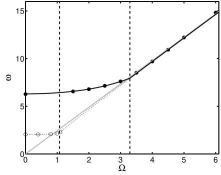
Figure 1: Frequency of the lowest $m=0$ mode as a function of the angular velocity $\Omega$ (in units of the trap frequency) for $g=1000$. The sum rule estimates (9) for $\lambda=0.5$ and $\lambda=10^{-3}$ are plotted as solid black and dotted lines respectively, while the results of solving the GP equation numerically are plotted as solid and open circles. The gray line is the asymptotic prediction $\omega=\sqrt{6}\Omega$ and the dashed lines represent the critical frequencies for hole formation, $\Omega_{h}$, for both values of $\lambda$.

Sum rules can also be applied to excitations of the form $f=r^{|m|}e^{im\phi}$, which carry multipolarities different from zero. We consider the moments $m_{1}^{+}(F)=m_{1}(F)+m_{1}(F^{\dagger})$ and $m_{3}^{+}(F)=m_{3}(F)+m_{3}(F^{\dagger})$. These can be easily expressed in terms of commutators as $m_{1}^{+}(F)=\langle{[F^{\dagger},[H,F]]}\rangle$ and $m_{3}^{+}(F)=\langle{[[F^{\dagger},H],[H,[H,F]]]}\rangle$. From the previous expressions for the dipole ($m=1$) and quadrupole ($m=2$) operators $\mathcal{D}$ and $\mathcal{Q}$, and using the Thomas-Fermi approximation footnote:TF for $\Omega\geq\Omega_{h}$ one predicts the following results for the ratio between the cubic and energy weighted sum rules

$$\frac{m_{3}^{+}(\mathcal{D})}{m_{1}^{+}(\mathcal{D})} = 5\Omega^{2}-1\ ,$$ (10)

$$\frac{m_{3}^{+}(\mathcal{Q})}{m_{1}^{+}(\mathcal{Q})} = 5\Omega^{2}-1+\frac{3}{5}\frac{\lambda^{2}R_{-}^{4}}{\Omega^{2}-1}\ .$$ (11)

In the large $\Omega$ limit Eqs. (10) and (11) both yield $\sqrt{5}\Omega$ for the excitation frequency, which does not coincide with the prediction of Eq. (7). This result, which is inconsistent with a one-mode assumption, reveals the existence of additional modes not described by Eq. (6). Indeed, assuming that $m_{3}^{+}$ is exhausted by the $j=1$ modes, the fact that the ratio $m_{3}^{+}/m_{1}^{+}$ is smaller than the corresponding frequency $\sqrt{6}\Omega$ implies that $m_{1}^{+}$ includes contributions from lower frequency modes. In particular one concludes that the latter account for $1/6$ of the total $m_{1}^{+}$ moment.

The $\Omega$ dependence of these lowest frequency modes can be simply inferred from Eq. (5) where, neglecting higher order corrections, one finds that the frequency should be proportional to $|m|\lambda R^{2}_{-}/\Omega$. These modes can be interpreted as describing a sound wave directed along the azimuthal direction, in contrast to the high-lying modes which correspond to a radial shape oscillation of the annulus. The coefficient of proportionality can be estimated from the ratio between the energy and inverse energy weighted sum rules. The low-lying modes contribute only $1/6$ of the $m_{1}^{+}$ moment; the $m_{-1}^{+}$ sum rule, which is expected to be exhausted by the low lying modes, is given by the static response $\chi$. In the large $\Omega$ limit, the linearized hydrodynamic equations with a multipole perturbation give $m_{-1}^{+}=-\chi=(N\pi/g)R_{-}^{2}(\Omega^{2}/2\lambda)^{|m|}$. Since $m_{1}^{+}\sim 2Nm^{2}(\Omega^{2}/2\lambda)^{|m|-1}$ in the same limit, we find the frequency $\omega=(m_{1}^{+}/6m_{-1}^{+})^{1/2}=(\sqrt{2}/6)|m|\lambda R^{2}_{-}/\Omega$. The same result can also be derived using a variational analysis of Eq. (5). It is also worth noticing that $\omega\propto\lambda^{2/3}$ tends to zero in the $\lambda\to 0$ limit.

Fig. 2 shows a comparison between the analytical and numerical results for the high-lying and low-lying dipole and quadrupole modes. One sees good agreement between the two datasets at high $\Omega$, validating the sum rule approach used here. In the numerical simulations, the high-lying modes depart from the $\sqrt{6}\Omega$ dependence for $\Omega<\Omega_{h}$. The behavior at small $\Omega$ is qualitatively similar to the one exhibited in a rotating harmonic trap, where only one mode per branch is present. In particular for $\lambda\ll 1$ and $\Omega<1$ the equations of rotational hydrodynamics in the rotating frame give the result stripes ; JILA quadrupole $\omega(m=\pm 2)=\sqrt{2-\Omega^{2}}\mp\Omega$ for the two quadrupole frequencies, while for the dipole one has $\omega(m=\pm 1)=1\mp\Omega$. At large $\Omega$, the numerical results also show that the low-lying quadrupole mode frequency is larger than that of the dipole mode by a factor of two, in agreement with the arguments presented above.

The excitation energies in the laboratory frame are related to those in the rotating frame by $E_{\text{lab}}=E_{\text{rot}}+m\Omega$. For a proper identification of the modes in the lab frame, it is crucial to consider the sign of the azimuthal quantum number $m$ associated with each excitation. For this purpose it is useful to evaluate the strengths $\sigma^{+}=|\langle{n|F|0}\rangle|^{2}$ and $\sigma^{-}=|\langle{n|F^{\dagger}|0}\rangle|^{2}$, relative to the operators $F$ and $F^{\dagger}$ exciting states with angular momentum $\pm m$. A careful analysis of the response function reveals that the upper quadrupole level corresponds to an $m=-2$ mode, the $m=+2$ strength relative to this level being extremely small. A different situation takes place for the low-lying level. When $\Omega<1$ this level has mainly an $m=+2$ character, as in the case of Ref. stripes . For $\Omega>\Omega_{h}$, instead, both the $m=\pm 2$ strengths significantly differ from zero. For example, at $\Omega=5$ and for the parameters of Fig. 2, the numerical simulation shows that $\sigma_{\text{H}}^{+}\simeq 0$, $\sigma_{\text{H}}^{-}=12.0N$, $\sigma_{\text{L}}^{+}=19.9N$, $\sigma_{\text{L}}^{-}=7.8N$, where $\sigma_{\text{H,L}}^{\pm}$ are the strengths associated with the high and low-lying $m=\pm 2$ modes. In conclusion, we predict that in the lab frame for $\Omega>\Omega_{h}$ one should observe two $m=-2$ modes with frequencies $\omega_{\text{H}}-2\Omega$ and $|\omega_{\text{L}}-2\Omega|$, and one $m=+2$ mode with frequency $\omega_{\text{L}}+2\Omega$, where $\omega_{\text{H,L}}$ are the high and low-lying frequencies in the rotating frame modes . We also notice that at high angular velocity the $m=-2$ mode with frequency $|\omega_{\text{L}}-2\Omega|$ is energetically unstable in the lab frame. Similar results are found for the dipole modes.

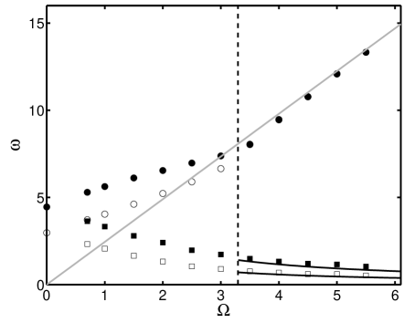
Figure 2: Numerical results for the high-lying (circles) and low-lying (squares) $|m|=1$ (open) and $|m|=2$ (closed) mode frequencies as a function of the angular velocity $\Omega$ (in units of the trap frequency), for $g=1000$ and $\lambda=0.5$. These are compared to the analytical results, where solid lines show the sum rule estimates for the low-lying modes while the gray line is the asymptotic prediction $\omega_{\text{H}}=\sqrt{6}\Omega$ expected to hold at large $\Omega$. The vertical dashed line denotes the value of $\Omega_{h}$.

We finally discuss the case of the giant vortex equilibrium configuration, where the velocity field of the condensate is irrotational. In this case, linearizing the Gross-Pitaevskii equation in the rotating frame gives two coupled equations for the density and the phase variations $\delta{n}$ and $\delta{S}$

$$\!\!\!\!\!\!\!\!\!\frac{\partial}{\partial t}\,\delta{n}+\left(\frac{v_{\rm irr}}{r}-\Omega\right)\frac{\partial\delta n}{\partial\phi}+\bm{\nabla}\cdot({n}_{0}\,\bm{\nabla}\delta S)=0\,,$$ (12)

$$\!\!\!\!\!\!\!\!\!\frac{\partial}{\partial t}\,\delta S+\left(\frac{v_{\rm irr}}{r}-\Omega\right)\frac{\partial\delta S}{\partial\phi}+g\delta n=0\,,$$ (13)

where $v_{\rm irr}=\nu/r$ for a giant vortex with circulation $\nu$ equilibrium . From these equations one can derive an equation similar to Eq. (5), but for the phase rather than the density. For large $\Omega$, the solutions are again Legendre polynomials, but with eigenfrequencies $\omega^{2}=3j(j+1)\Omega^{2}$ where $j\geq 1$. Hence the $j=1$ mode has the same frequency for both the irrotational and solid body cases, but the frequencies for the $j>1$ modes are different. In the case of the low-lying modes for $m\neq 0$, using the sum rule or hydrodynamic methods discussed earlier, we find a frequency that has the same $1/\Omega$ dependence as in the vortex lattice case, but is larger by a factor $3^{1/6}$.

In summary, we have studied normal modes of a Bose condensate in a harmonic plus quartic potential using analytic methods (hydrodynamic equations and sum rule) and numerical solution of the Gross-Pitaevskii equation. At large angular velocities $\Omega$ we find a radial mode with a frequency $\sqrt{6}\Omega$ independent of the mode multipolarity and value of $\lambda$, as well as low-lying modes corresponding to waves around the annular condensate.

This research was supported by the Ministero dell’Istruzione, dell’Università e della Ricerca. Some of the work was performed at the Kavli Institute for Theoretical Physics, supported in part by the National Science Foundation under Grant No. PHY99-0794.

References

- (1) V. Bretin, S. Stock, Y. Seurin, and J. Dalibard, Phys. Rev. Lett. 92, 050403 (2004); S. Stock, V. Bretin, F. Chevy, and J. Dalibard, Europhys. Lett. 65, 594 (2004).
- (2) A.L. Fetter, Phys. Rev. A 64, 063608 (2001); U.R. Fischer and G. Baym, Phys. Rev. Lett. 90, 140402 (2003); G.M. Kavoulakis and G. Baym, New J. Phys. 5, 51.1 (2003); E. Lundh, Phys. Rev. A 65, 043604 (2002); A.D. Jackson, G.M. Kavoulakis, and E. Lundh, Phys. Rev. A 69, 053619 (2004); A.D. Jackson and G.M. Kavoulakis, Phys. Rev. A 70, 023601 (2004).
- (3) A.L. Fetter, B. Jackson, and S. Stringari, cond-mat/0407119.
- (4) M. Cozzini and S. Stringari, Phys. Rev. A 67, 041602(R) (2003).
- (5) The solution is rejected due to its unphysical nature. Indeed, for the case this solution does not conserve the particle number, while for it gives rise to a divergent velocity field at the condensate boundaries.
- (6) The result can also be found within the hydrodynamic formalism by solving Eq. (5) perturbatively with respect to .
- (7) For the dipole operator one finds and , while for the quadrupole one instead has and , where and . In the Thomas-Fermi diffused vorticity approach the equilibrium velocity is , so that and .
- (8) The result for the quadrupole frequencies has been confirmed in the experiment of P.C. Haljan, I. Coddington, P. Engels, and E.A. Cornell, Phys. Rev. Lett. 87, 210403 (2001), where a harmonic trap was employed.
- (9) This scenario is based on the assumption that in the rotating frame only two levels (high and low-lying) are excited by the operators and . Numerical integration of Eq. (5) actually shows the occurrence of a very small splitting between the low-lying modes, which however barely affects the main results of the present analysis.