Also at ]the Jawaharlal Nehru Centre for Advanced Scientific Research, Bangalore, India.

Drag Reduction by Polymer Additives in Decaying Turbulence

Abstract

We present results from a systematic numerical study of decaying turbulence in a dilute polymer solution by using a shell-model version of the FENE-P equations. Our study leads to an appealing definition of drag reduction for the case of decaying turbulence. We exhibit several new results, such as the potential-energy spectrum of the polymer, hitherto unobserved features in the temporal evolution of the kinetic-energy spectrum, and characterize intermittency in such systems. We compare our results with the GOY shell model for fluid turbulence.

The phenomenon of drag reduction by polymer additivesLumley , whereby dilute solutions of linear, flexible, high-molecular-weight polymers exhibit frictional resistance to flow much lower than that of the pure solvent, has almost exclusively been studied within the context of statistically steady turbulent flows since the pioneering work of TomsToms . By contrast, there is an extreme scarcity of results concerning the effects of polymer additives on decaying turbulenceNadolink . Experimental studies of decaying, homogeneous turbulence behind a grid indicate, for such dilute polymer solutions, a turbulent energy spectrum similar to that found without polymersFriehe ; Mccomb . However, flow visualization via die-injection tracersMccomb and particle image velocimetryDoorn show an inhibition of small-scale structures in the presence of polymer additives. To the best of our knowledge decaying turbulence in such polymer solutions has not been studied numerically. We initiate such a study here by using a shell model that is well suited to examining the effects of polymer additives in turbulent flows that are homogeneous and in which bounding walls have no direct role. We obtain several interesting results including a natural definition of the percentage drag-reduction $DR$, which has been lacking for the case of decaying turbulence. We show that the dependence of $DR$ on the polymer concentration $c$ is in qualitative accord with experimentsLumley as is the suppression of small-scale structures which we quantify by obtaining the filtered-wavenumber-dependence of the flatness of the velocity field.
We will use a shell-model version of the FENE-P (Finitely Extensible Nonlinear Elastic - Peterlin)Warner ; Bird model for dilute polymer solutions that has often been used for studying viscoelastic effects since it contains the basic characteristics of molecular stretching, orientation and finite extensibility seen in polymer molecules. A direct numerical simulation of the FENE-P equations is computationally prohibitive. This motivates the use of a shell model that captures the essential features of the FENE-P equations. Recent studiesBenzi have exploited a formal analogyFouxon of the FENE-P equations with those of magnetohydrodynamics (MHD) to construct such a shell model. We investigate decaying turbulence in a dilute polymer solution by developing a similar shell model for the FENE-P equations. The unforced FENE-P equationsWarner ; Bird are

$$\frac{\partial{\bf v}}{\partial{t}}+({\bf v\cdot\bigtriangledown}){\bf v}=-\frac{\bigtriangledown p}{\rho_{s}}+\nu_{s}{\bigtriangledown^{2}\bf v}+\bigtriangledown\cdot{\cal T},$$ (1)

$$\begin{split}\frac{\partial{\cal R}_{\alpha\beta}}{\partial t}+({\bf v\cdot\bigtriangledown}){\cal R}_{\alpha\beta}=&\frac{\partial v_{\alpha}}{\partial x_{\gamma}}{\cal R}_{\gamma\beta}+\\ &{\cal R}_{\alpha\gamma}\frac{\partial v_{\beta}}{\partial x_{\gamma}}-\frac{1}{\nu_{p}}{\cal T}_{\alpha\beta},\end{split}$$

where $p$ is the pressure, $\nu_{s}$ the kinematic viscosity of the solvent, $\nu_{p}$ a ‘viscosity’ parameter, $\rho_{s}$ the density of the solvent, incompressibility is enforced via $\bigtriangledown\cdot{\textbf{v}}=0$, and the polymer conformation tensor is ${\cal R}_{\alpha\beta}\equiv\langle R_{\alpha}R_{\beta}\rangle/R_{0}^{2}$, with the angular brackets indicating an average over polymer configurations, of the dyadic product of the end-to-end vector R(x,t) of the polymer molecules. The maximal extension of the polymer molecules is restricted by the condition $\langle R_{\gamma}^{2}\rangle<R_{0}^{2}$. The contribution to the stress tensor because of the polymer is ${\cal T}_{\alpha\beta}=\nu_{p}[P({\bf x},t){\cal R}_{\alpha\beta}-\delta_{\alpha\beta}]/\tau_{p}$, with $\delta_{\alpha\beta}$ the Kronecker delta, $\tau_{p}$ the time constant of the FENE-P model, and $P({\bf x},t)\equiv 1/(1-{\cal R}_{\gamma\gamma})$ (with repeated indices indicating a trace). The concentration of the polymer is parametrized here by $c\equiv\nu_{p}/\nu_{s}$.
Our shell-model version of the unforced FENE-P equations, obtained by generalising a shell model originally proposed for three-dimensional MHDFrick , is

$$\frac{dv_{n}}{dt} = \Phi_{n,vv}-\nu_{s}k^{2}_{n}v_{n}+\frac{\nu_{p}}{\tau_{p}}P(b)\Phi_{n,bb},$$

$$\frac{db_{n}}{dt} = \Phi_{n,vb}-\Phi_{n,bv}-\frac{1}{\tau_{p}}P(b)b_{n},$$ (2)

where $P(b)\equiv 1/(1-\sum_{n}|b_{n}|^{2})$, $v_{n}$ and $b_{n}$ are complex, scalar variables representing the velocity and the (normalized) polymer end-to-end vector fields, respectively, with the discrete wavenumbers $k_{n}=k_{0}2^{n}$ ($k_{0}$ sets the scale for wave-numbers), for shell index $n$ ($n=1\ldots N$, for $N$ shells), with $\Phi_{n,vv}=i(a_{1}k_{n}v_{n+1}v_{n+2}+a_{2}k_{n-1}v_{n+1}v_{n-1}+a_{3}k_{n-2}v_{n-1}v_{n-2})$, $\Phi_{n,bb}=-i(a_{1}k_{n}b_{n+1}b_{n+2}+a_{2}k_{n-1}b_{n+1}b_{n-1}+a_{3}k_{n-2}b_{n-1}b_{n-2})$, $\Phi_{n,vb}=i(a_{4}k_{n}v_{n+1}b_{n+2}+a_{5}k_{n-1}v_{n-1}b_{n+1}+a_{6}k_{n-2}v_{n-1}b_{n-2})$, and $\Phi_{n,bv}=-i(a_{4}k_{n}b_{n+1}v_{n+2}+a_{5}k_{n-1}b_{n-1}v_{n+1}+a_{6}k_{n-2}b_{n-1}v_{n-2})$. As in Ref. Frick we choose $a_{1}=1$, $a_{2}=a_{3}=-1/2$, $a_{4}=1/6$, $a_{5}=1/3$, and $a_{6}=-2/3$. We solve Eqs. (2) numerically by using an Adams-Bashforth schemePisarenko and double-precision arithmetic, with a step size $\delta t=10^{-2}$ and $N=22$ shells, with $k_{0}=1/16$ and $\nu_{s}=10^{-3}$. For all our runs (except those in FIGs. 3 and 4) we set $c=100$. For numerical stability we add a nominal viscous term $-\nu_{b}k_{n}^{2}b_{n}$ to the shell-model equations for $b_{n}$ and set $\nu_{b}/\nu_{s}=10^{-13}$. With these parameter values, our code is stable for $1.0<\tau_{p}<7.8$, and we observe that the corresponding percentage drag reduction $DR$ (see below) lies in the range $63\%<DR<98\%$. For specificity we use $\tau_{p}=2.1$ for the data presented here. The initial velocity field is taken to be $v_{n}^{0}=k_{n}^{1/2}e^{i\theta_{n}}$ (for $n=1,2$), $v_{n}^{0}=k_{n}^{1/2}e^{-k_{n}^{2}}e^{i\theta_{n}}$ (for $3\leq n\leq N$) and the initial polymer field to be $b_{n}^{0}={k_{n}}^{1/2}e^{i\phi_{n}},$ with $\theta_{n}$ and $\phi_{n}$ independent random phases distributed uniformly between $0$ and $2\pi$. In decaying turbulence, it is convenient to measure time in units of the initial large eddy-turnover time. For our shell model this is $\tau_{0}\equiv 1/(v_{rms}^{0}k_{1})$ with $v_{rms}^{0}\equiv[\langle\sum_{n}|v_{n}^{0}|^{2}\rangle]^{1/2}$, the root-mean-square value of the initial velocity (we find $\tau_{0}=5.2$). We use the dimensionless time $\tau\equiv t/\tau_{0}$ ($t$ is the product of the number of steps and $\delta t$). Our runs are ensemble averaged over $10^{4}$ independent initial conditions with different realizations of phases. We define $Re_{v}^{0}\equiv v^{0}_{rms}/(k_{1}\nu_{s})$ to be the value of the initial Reynolds number (here $Re_{v}^{0}$ equals $12309$). Shell-model energy densities are defined as $E_{a}(k_{n})\equiv\langle|a_{n}|^{2}/k_{n}\rangle$, with $a=v$ for the velocity fieldFrick ; GOY and $a=b$ for the polymer field. Equations (2) reduce to those for the Gledzer-Ohkitani-Yamada (GOY) shell modelGOY when the polymer-field terms are suppressed. For our GOY shell model runs, we use initial parameter values as for the FENE-P shell model to facilitate comparisons between the two.

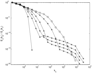
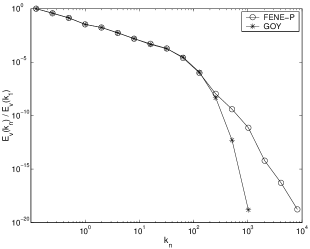
Figure 1: (a) Log-log plots of the temporal evolution of the normalized kinetic energy spectra $E_{v}(k_{n})/E_{v}(k_{1})$ of the FENE-P shell model as a function of the wavenumber $k_{n}$. The plot with open circles is calculated at cascade completion.
(b) Log-log plots of the normalized kinetic energy spectra $E_{v}(k_{n})/E_{v}(k_{1})$ as a function of the wavenumber $k_{n}$ for the FENE-P and the GOY shell models at cascade completion. The observed slope is $-1.67\pm 0.01$ for the range $0.25<k_{n}<64$.

Figure 1(a) shows the time evolution of the normalized kinetic energy spectrum $E_{v}(k_{n})/E_{v}(k_{1})$ (successive curves separated by time intervals of $0.2\tau$). We see a cascade of the energy to large wavenumbers after which the shape of the spectrum does not change appreciably but the energy decays. We observe the evolution of a flat portion in the spectrum that vanishes upon cascade completion (plot with open circles). Figure 1(b) compares kinetic-energy spectra at cascade completion for our model (Eqs. (2)) and for the GOY shell model. In the inertial range, both spectra are indistinguishable and show a Kolmogorov-type $k^{-5/3}$ behavior with an observed slope of $-1.67\pm 0.01$ (with errors from least-square fits), a result consistent with experimentsFriehe ; Mccomb of decaying, homogeneous turbulence behind a grid for a dilute polymer solution. However, significant differences show up in the dissipation range: the spectrum for the FENE-P shell model falls much more slowly than its GOY-model counterpart indicating greatly reduced dissipation at large wavenumbers. ExperimentalFriehe ; Mccomb energy spectra do not cover as large a range of spatial scales as we can cover in our shell-model study, and thus, to the best of our knowledge, these dissipation-range discrepancies of the energy spectra, with and without polymer additives, have not been noticed earlier. We note that our results in FIG. 1(b) distinctly differ from corresponding resultsBenzi for statistically steady turbulence, where a tilt in the spectrum has been observed at low wavenumbers in the FENE-P shell model relative to that obtained from the GOY shell model.

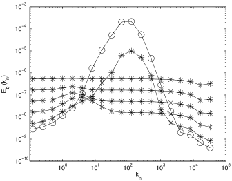
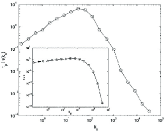
Figure 2: (a) Log-log plots of the temporal evolution of the potential energy spectrum $E_{b}(k_{n})$ of the polymer field as a function of the wavenumber $k_{n}$. The plot with open circles is calculated at cascade completion.
(b) Log-log plot of the ratio of the time constant $\tau_{p}$ of the FENE-P shell model and the turbulence time-scale $\tau(k_{n})$ as a function of the wavenumber $k_{n}$ at cascade completion. The inset shows the inverse of the turbulence time-scale $\tau(k_{n})$ as a function of the wavenumber $k_{n}$ for the GOY shell model at cascade completion.

In FIG. 2(a), we display the time evolution of the potential-energy spectrum of the polymer $E_{b}(k_{n})$ (with a temporal separation of $0.2\tau$). Starting from an initially flat spectrum, we observe the appearance and subsequent growth of a protuberance that bulges out maximally on cascade completion (plot with open circles) at a wavenumber corresponding to the value, of order unity, of the ratio of the polymer time constant $\tau_{p}$ and the turbulence time scale $\tau(k_{n})\equiv 1/(k_{n}|v(k_{n})|)$ (FIG. 2(b)). The result is in agreement with a hypothesis (for statistically steady turbulence) in Ref. Degennes wherein a polymer molecule, immersed in an eddy with a turbulent time-scale comparable to the polymer relaxation time, undergoes a ‘coil-stretch’ transition with an increment in the potential-energy spectrum at the wavenumber corresponding to the inverse of the eddy size. The inset in FIG. 2(b) is a plot of the inverse of the turbulence time-scale $\tau(k_{n})$ as a function of the wavenumber $k_{n}$ for the GOY shell model. In both plots, within the inertial range, $\tau(k_{n})\sim k_{n}^{-2/3}$, a result consistent with the $-5/3$ power-law in the kinetic energy spectrum.
A log-log plot of the normalized kinetic energy dissipation rate ${\mathcal{E}}_{f}/{\mathcal{E}}_{f,0}$ of the FENE-P shell model versus dimensionless time $\tau$ for different values of $c$ is shown in FIG. 3 (with ${\cal E}_{f}/{\cal E}_{f,0}\equiv\langle\sum_{n}k_{n}^{2}|v_{n}|^{2}\rangle/\langle\sum_{n}k_{n}^{2}|v_{n}^{0}|^{2}\rangle$, the additional index $0$ indicating values calculated at initial times). The reduction in the peak value with respect to the value at initial times, with increasing concentration, is indicative of an enhanced value of the stored elastic potential energy in the polymer molecules due to their extension. The analogous plot for the GOY shell model is identical to the plot for $c=10$ in FIG. 3. We are therefore led to the following natural definition of the percentage drag reduction $DR$ for decaying turbulence:

$$DR\equiv\Big{(}\frac{{\cal E}_{g,m}/{\cal E}_{g,0}-{\cal E}_{f,m}/{\cal E}_{f,0}}{{\cal E}_{g,m}/{\cal E}_{g,0}}\Big{)}\times 100,$$ (3)

where the kinetic energy dissipation rates ${\cal E}_{a}\equiv\langle\sum_{n}k_{n}^{2}|v_{n}|^{2}\rangle$ (the subscript $a=f$ for the FENE-P shell model and $a=g$ for the GOY shell model) are calculated upon cascade completion when the dissipation rate is a maximum (indicated by an additional subscript $m$) and normalized by their values at initial times (indicated by an additional subscript $0$). With the choice of initial parameter values as specified above, ${\mathcal{E}}_{g,m}/{\cal E}_{g,0}$ equals $234.96\pm 0.01$.

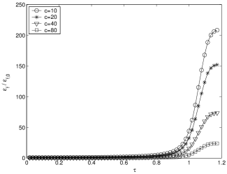
Figure 3: The normalized kinetic energy dissipation rate ${\mathcal{E}}_{f}/{\mathcal{E}}_{f,0}$ of the FENE-P shell model as a function of the dimensionless time $\tau$ for different values of concentration $c$, as specified in the legend.

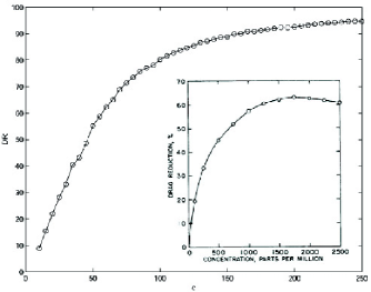
Figure 4: Plot of the percentage drag reduction $DR$ (Eq. (3)) as a function of the concentration $c$. The inset shows a plot for the same quantities taken from Ref. Hoyt (see the text for definitions).

In FIG. 4, we use Eq. (3) to plot $DR$ as a function of $c$. The inset figure from Ref. Hoyt is a similar plot for a dilute solution of Carrageenanfn (a seaweed derivative) in a pipe-flow Reynolds number of $14000$. The qualitative agreement with a laboratory experiment (for statistically steady turbulence) supports our definition of drag reduction for decaying turbulence.

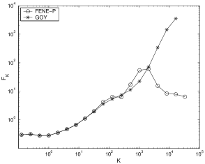
Figure 5: Plot of the flatness $F_{K}$ as a function of the filtered wavenumber $K$ (see the text for definitions) at cascade completion for the FENE-P and the GOY shell models.

Laboratory experiments in both statistically steadyDam and decayingMccomb ; Doorn turbulent flows of dilute polymer solutions show an inhibition of small-scale structures and narrower probability distribution functions of velocity differencesDam . We plot in FIG. 5, the flatness $F_{K}\equiv\langle|v^{>}_{K}|^{4}\rangle/\langle|v^{>}_{K}|^{2}\rangle^{2}$ ($\langle|v^{>}_{K}|^{4}\rangle\equiv\langle\sum_{n}|v_{n}|^{4}\rangle$, $\langle|v^{>}_{K}|^{2}\rangle\equiv\langle\sum_{n}|v_{n}|^{2}\rangle$, with $n=K...N$), $K=1...N$, as a function of the ‘filtered’Frisch wavenumber $K$ for the FENE-P and the GOY shell models at cascade completion. We observe that, in the GOY shell model, the flatness $F_{K}$ exhibits unbounded growth for large wavenumbers, an indication of strong intermittency in the dissipation scales. However, for the FENE-P shell model, we observe that the flatness is greatly reduced relative to that for GOY and, in fact, decreases in the dissipation scales. Our results are consistent, therefore, with laboratory experiments which show a suppression of small structures that would imply reduced intermittency in the dissipation range of our shell model.
Laboratory experimentsMccomb ; Doorn of decaying turbulence behind grids indicate a reduced decay rate of the kinetic energy in a dilute polymer solution, relative to the pure solvent. In the initial period of decay, before the integral scale of turbulence becomes of the order of the size of the system (the minimum wavenumber, in the case of shell models), we observe a decay rate of $-1.80\pm 0.01$ for the FENE-P shell model and a decay rate of $-2.01\pm 0.02$ for the GOY shell model (a result consistent with Ref. Lohse ).
In conclusion, then, we have presented results from a systematic numerical study of decaying turbulence in a dilute polymer solution by employing a shell-model for the FENE-P equations. This leads to a natural definition of drag reduction for such a system and new results on the potential- and kinetic energy spectra which are in qualitative agreement with experimental findings.

- (1) J. Lumley, J. Polym. Sci.:Macromolecular Reviews, 7, 263 (1973); P. Virk, AIChE J., 21, 4, 625 (1975).
- (2) B. Toms, Proceedings of First International Congress on Rheology, Section II, 135 (North-Holland, Amsterdam, 1949).
- (3) R. Nadolink and W. Haigh, ASME Appl. Mech. Revs., 48, 351 (1995).
- (4) C. Friehe and W. Schwarz, J. Fluid Mech., 44, 1, 173 (1970).
- (5) W. McComb, J. Allan, and C. Greated, Phys. Fluids, 20, 6, 873 (1977).
- (6) E. van Doorn, C. White, and K. Sreenivasan, Phys. Fluids, 11, 8, 2387 (1999).
- (7) H. Warner, Ind. Eng. Chem. Fundamentals, 11, 3, 379 (1972); R. Armstrong, J. Chem. Phys., 60, 3, 724 (1974); A. Peterlin, J. Polym. Sci., Polym. Lett., 4, 4, 287 (1966).
- (8) R. Bird, C. Curtiss, R. Armstrong and O. Hassager, Dynamics of Polymeric Liquids, 2 (Wiley, New York, 1987).
- (9) R. Benzi, E. Angelis, R. Govindarajan, and I. Procaccia, Phys. Rev. E, 68, 016308 (2003); R. Benzi, E. Ching, N. Horesh, and I. Proccacia, Phys. Rev. Lett., 92, 078302 (2004).
- (10) A. Fouxon and V. Lebedev, Phys. Fluids, 15, 7, 2060 (2003).
- (11) P. Frick and D. Sokoloff, Phys. Rev. E, 57, 4155 (1998); A. Basu, A. Sain, S. Dhar, and R. Pandit, Phys. Rev. Lett., 81, 2687 (1998). For illustrative decay studies see C. Kalelkar and R. Pandit, Phys. Rev. E, 69, 046304 (2004).
- (12) E. Gledzer, Sov. Phys. Dokl., 18, 216 (1973); K. Ohkitani and M. Yamada, Prog. Theor. Phys., 81, 329 (1989); L. Kadanoff, D. Lohse, J. Wang, and R. Benzi, Phys. Fluids, 7, 517 (1995).
- (13) D. Pisarenko, L. Biferale, D. Courvoisier, U. Frisch, and M. Vergassola, Phys. Fluids A, 56, 10, 2533 (1993).
- (14) P. De Gennes, J. Chem. Phys., 60, 12, 5030 (1974).
- (15) J. Hoyt, Progress in Astronautics and Aeronautics, 123, 418 (American Institute of Astronautics and Aeronautics, Washington, D.C., 1990), reprinted with permission. Here, , where is the pressure drop in a given length of the pipe, the subscript for the pure solvent and for the dilute polymer solution, with the same flow rate of the liquid.
- (16) Our choice of polymer is merely representative and not meant to characterise any specific polymer.
- (17) P. van Dam, G. Wegdam, and J. van der Elsken, J. Non-Newtonian Fluid Mech., 53, 215 (1994).
- (18) U. Frisch, Turbulence: The Legacy of A. N. Kolmogorov, (Cambridge University Press, Cambridge, 1996).
- (19) J. Hooghoudt, D. Lohse, and F. Toschi, Phys. Fluids, 13, 7, 2013 (2001).