Long range frustration in finite connectivity spin glasses: A mean field theory and its application to the random $K$-satisfiability problem

Abstract

A mean field theory of long range frustration is constructed for spin glass systems with quenched randomness of vertex–vertex connections and of spin–spin coupling strengths. This theory is applied to a spin glass model of the random $K$-satisfiability problem ($K=2$ or $K=3$).

The satisfiability transition in a random $2$-SAT formula occurs when the clauses-to-variables ratio $\alpha$ approaches $\alpha_{c}(2)=1$. However, long range frustration among unfrozen variable nodes builds up only when $\alpha>\alpha_{R}(2)=4.4588$. For the random $3$-SAT problem, we find a long–range frustrated mean field solution when $\alpha>\alpha_{R}(3)=4.1897$. The long range frustration order parameter $R$ of this solution jumps from zero to a finite positive value at $\alpha_{R}(3)$, while the energy density increases only gradually from zero as a function of $\alpha$. The SAT–UNSAT transition point of this solution is lower than the value of $\alpha_{c}(3)=4.267$ obtained by the survey propagation algorithm. Two possible reasons for this discrepancy are suggested.

The zero–temperature phase diagram of the $\pm J$ Viana–Bray model is also determined, which is identical to that of the random $2$-SAT problem. The predicted phase transition between a non-frustrated and a long–range frustrated spin glass phase might also be observable in real materials at a finite temperature.

[published in New Journal of Physics 7 (2005) 123; freely available at http://www.njp.org/]

I Introduction

An attempt was made in a recent paper Zhou (2004) to study the vertex cover problem from the viewpoint of long range frustration. The vertex cover problem, sometimes also referred to as the hard–core gas condensation problem in the physics literature, can be mapped to a spin glass model with quenched randomness coming from the underlying random vertex–vertex connection patterns. In the present paper, we extend the basic idea and the method of Ref. Zhou (2004) to spin glass systems with an additional kind of quenched randomness due to the random couplings among interacting vertices. We demonstrate our calculations by working on a spin glass model of the random $K$-satisfiability ($K$-SAT) problem. Our results will be compared with known algorithmic and analytical conclusions.

The $K$-SAT is at the root of computational complexity Garey and Johnson (1979). A $K$-SAT formula involves $N$ Boolean variables and $M=\alpha N$ constraints or clauses, each of which is a disjunction of $K$ Boolean variables or their negations. The parameter $\alpha$ is called the clauses-to-variables ratio. A $K$-SAT formula is satisfiable (SAT) if there exists at least one assignment of the Boolean variables (a solution) such that all clauses are satisfied; otherwise it is unsatisfiable (UNSAT). For example, the $2$-SAT formula

$$(x_{1}\lor\bar{x_{2}})\land(x_{1}\lor x_{2})\land(\bar{x_{1}}\lor x_{3})\land(x_{2}\lor\bar{x_{3}})$$

with $N=3$ and $M=4$ has a SAT solution of $x_{1}=x_{2}=x_{3}={\tt TRUE}$. Given a $K$-SAT formula, the objective is to judge whether it is satisfiable or not, and if it is, to find a satisfying solution. The satisfiability of a $2$-SAT formula can be determined in a run time that scales linearly with the number $N$ of Boolean variables Aspvall et al. (1979). However, to determine the satisfiability of a $K$-SAT formula with $K\geq 3$ is NP-complete, with a computation time that scales exponentially with $N$ in the worst case. The reason for this qualitative difference in computational complexity is still not completely clear.

When a $K$-SAT formula of $N$ variables and $M$ clauses is chosen randomly from the ensemble of all such formulas, it was observed Cheeseman et al. (1991); Kirkpatrick and Selman (1994); Crawford and Auton (1996) that its probability $p$ of being satisfiable drops from $p\approx 1$ to $p\approx 0$ over a small range of the parameter $\alpha$ around certain $\alpha_{c}$ (for $K=3$, $\alpha_{c}\approx 4.2$ Kirkpatrick and Selman (1994); Crawford and Auton (1996); Achlioptas (2001)). Furthermore, although the $K$-SAT problem ($K\geq 3$) in general is NP-complete, the satisfiability of a randomly chosen formula can often be easily determined by a heuristic algorithm, provided that its parameter $\alpha$ is not at the vicinity of the SAT-UNSAT transition point $\alpha_{c}$. The really difficult instances of random $K$-SAT ($K\geq 3$) are located at the parameter regime of $\alpha\approx\alpha_{c}$ Cheeseman et al. (1991).

The above mentioned threshold phenomena are reminiscent of what is usually observed in a physical system around its phase transition or critical point. Concepts of spin glass physics, such as replica symmetry breaking and proliferation of metastable states, were applied to the random $K$-SAT problem in some recent articles Monasson and Zecchina (1996, 1997); Monasson et al. (1999); Mézard et al. (2002); Mézard and Zecchina (2002). For the random $3$-SAT problem, Mézard and co-authors Mézard et al. (2002); Mézard and Zecchina (2002) found that in the parameter regime of $3.921<\alpha<4.267$, there exists a hard-SAT phase with positive structural entropy (complexity). A random $3$-SAT formula in this phase is satisfiable by exponentially many Boolean configurations, which are clustered into different macroscopic domains. There are also exponentially many metastable domains of configurations which satisfy most but not all the clauses (a local search algorithm is likely to be trapped in one of these metastable configurational domains). This physical insight is implemented in an efficient heuristic survey propagation algorithm Braunstein et al. (2002) to find a solution for a random $3$-SAT formula.

Trying to understand more deeply the qualitative difference between the $2$-SAT and the general $K$-SAT problem ($K\geq 3$), in this paper we re-examine the random $2$-SAT and $3$-SAT problem by focusing on the issue of long range frustration among unfrozen Boolean variables. A long range frustration order parameter $R$ is calculated. We find that, while the SAT–UNSAT transition occurs at $\alpha_{c}(2)=1$ for the random $2$-SAT problem, long range frustration only gradually builds up when $\alpha\geq\alpha_{R}(2)=4.4588$, where the non-frustrated mean field solution becomes unstable. For the random $3$-SAT problem, we find a self-consistent long–range frustrated solution when $\alpha\geq\alpha_{R}(3)=4.189724$. The long range frustration order parameter $R$ of this solution jumps from zero to a finite positive value at $\alpha_{R}(3)$, while the energy density increases only gradually from zero as a function of $\alpha$. This solution predicts that the SAT-UNSAT transition occurs at $\alpha=\alpha_{R}(3)$. However, for the random $3$-SAT problem, the non-frustrated trivial mean field solution is stable even when $\alpha>\alpha_{R}(3)$; and furthermore, in the range of $3.921<\alpha<4.267$ there is a non-frustrated replica symmetry breaking solution of zero energy Mézard and Zecchina (2002). It is likely that the true SAT-UNSAT transition point is at $\alpha=\alpha_{c}(3)=4.267$. Two possible reasons for this discrepancy between our mean field solution and the solution of Ref. Mézard and Zecchina (2002) are discussed in this paper. It appears that, when the replica symmetry breaking occurs before the onset of long range frustration, the method outlined in this paper needs to be improved, and competitions among different macroscopic states should be considered in the mean field theory. More work is certainly needed to overcome this discrepancy.

This paper is organized as follows. We first define the random $K$-SAT problem in Sec. II. The random $2$-SAT problem and the $\pm J$ Viana–Bray spin glass model are then studied in Sec. III. The method developed in this section is then applied to the more difficult random $3$-SAT problem in Sec. IV. We summarize and discuss our main results in Sec. V.

II Spin glass model of the random $K$-satisfiability problem

We follow Ref. Mézard et al. (2002) and represent a random $K$-SAT formula by a random factor graph of $N$ variable nodes and $M=\alpha N$ function nodes. Each variable node $i$ represents a Boolean variable, with a spin value $\sigma_{i}=\pm 1$. It is connected to $k$ function nodes, where $k$ is a random integer governed by the Poisson distribution $f(k,c)$ of mean $c=K\alpha$. The Poisson distribution is defined as

$$f(k,c)={e^{-c}c^{k}\over k!}\ .$$ (1)

Each function node $a$ represents a clause (constraint); it is linked to $K$ randomly chosen variable nodes $i_{1},\ldots,i_{K}$. Function node $a$ has an energy $E_{a}$ which is either $0$ (clause satisfied) or $1$ (clause violated):

$$E_{a}=\prod\limits_{r=1}^{K}{1-J_{a}^{i_{r}}\sigma_{i_{r}}\over 2}\ ,$$ (2)

where $J_{a}^{i_{r}}$ is the edge strength between $a$ and $i_{r}$: $J_{a}^{i_{r}}=-1$ or $1$ depending on whether Boolean variable $i_{r}$ in clause $a$ is negated or not. In a given random $K$-SAT formula, $J_{a}^{i_{r}}$ is a quenched random variable with value equally distributed over $\pm 1$. The total energy of the system for each of the $2^{N}$ possible spin configurations is expressed as

$$E[\{\sigma_{i}\}]=\sum\limits_{a=1}^{M}E_{a}\ .$$ (3)

As we are interested in the ground–state energy landscape of model Eq. (3), only those configurations which have the global minimum energy are considered in later discussions.

III The random $2$-satisfiability problem and the $\pm J$ Viana–Bray spin glass model

We begin with the random $2$-SAT problem. Experience gained in this section will help us to understand the more difficult random $3$-SAT problem in the next section. We discuss the random $2$-SAT problem first from the viewpoint of long range frustration (Sec. III.1). Then we study it in Sec. III.2 through the cavity method of Mézard and Parisi Mézard and Parisi (2001, 2003) by setting the long range frustration order parameter to $R=0$. The later treatment causes an annoying divergence in the population dynamics, suggesting the necessity of taking into account the effect of long range frustration. In Sec. III.3 we briefly discuss the finite connectivity $\pm J$ Viana–Bray spin glass model.

III.1 Long range frustration in a single macroscopic state

The ground–state configurations of a random $2$-SAT formula may be classified into different macroscopic states Mézard and Parisi (2003) (hereafter, a macroscopic state is simply referred to as a state). Two microscopic configurations in the same state are mutually reachable by flipping a finite number of spins of one configuration and then letting the system relax. According to this definition of states, two configurations of the same state may differ from each other in the spin values of $O(N)$ variable nodes (this is due to the formation of a percolation cluster of unfrozen variable nodes discussed later). We focus on a randomly chosen macroscopic state $\beta$. In state $\beta$, the spin value of a randomly chosen variable node $i$ may be fixed to $\sigma_{i}\equiv+1$ (positively frozen), or to $\sigma_{i}\equiv-1$ (negatively frozen), or fluctuate over $\pm 1$ (unfrozen). The fraction of positively frozen, negatively frozen, and unfrozen variable nodes in state $\beta$ is, respectively, $q_{+}$, $q_{-}$, and $q_{0}$, with $q_{+}+q_{-}+q_{0}=1$. Our approach at the present stage is essentially replica symmetric because of the following reasons: (a) although many macroscopic states may coexist, our system is assumed to stay always in the same state,(b) a state is characterized by just two mean field parameters, $q_{0}$ and $R$ (to be defined later).

Since the spin values of the unfrozen variable nodes fluctuate among different configurations of state $\beta$, the possibility of correlation among these fluctuations must be taken into account. Consider an unfrozen variable node $i$. If its spin value is externally fixed to a prescribed value $\sigma_{i}=\sigma_{i}^{*}$ ($\sigma_{i}^{*}=\pm 1$ with equal probability), how many other unfrozen variable nodes must eventually fix their spins as a consequence?

For a random factor graph with size $N\to\infty$, the total number $s$ of affected variable nodes may scale linearly with $N$ and therefore also approaches infinity. If this happens, $\sigma_{i}^{*}$ is referred to as a canalizing value for variable node $i$, and variable node $i$ is referred to as type-I unfrozen with respect to spin value $\sigma_{i}^{*}$. This happens with probability $R$, with $R$ being our long range frustration order parameter. The total number of affected variable nodes may also be finite, $s\sim O(1)$. In this case, variable node $i$ is type-II unfrozen with respect to spin value $\sigma_{i}^{*}$. We emphasize that, if an unfrozen variable node $i$ is type-I unfrozen with respect to spin value say $\sigma_{i}=+1$, it is not necessarily also type-I unfrozen with respect to spin value $\sigma_{i}=-1$; in other words, the fact that $\sigma_{i}^{*}$ is a canalyzing value for variable node $i$ does not mean that $-\sigma_{i}^{*}$ is also a canalyzing value for the same node. In the remaining part of this article, to simplify the notation, we will frequently use phrases such as $``$variable node $i$ is type-I unfrozen” and $``$a type-II unfrozen variable node $i$”. It should be understood that, whenever we mention that a variable node $i$ is type-I or type-II unfrozen, we mean that it is type-I or type-II unfrozen with respect to a prescribed spin value $\sigma_{i}^{*}$.

Based on the bond percolation theory on random graphs Bollobás (1985), we know that the percolation clusters evoked by two type-I unfrozen variable nodes have a nonzero intersection of size proportional to $N$. Therefore, the spin values of all type-I unfrozen variable nodes must be strongly correlated. If we randomly choose two type-I unfrozen variable nodes $i$ and $j$, then with probability one half $\sigma_{i}^{*}$ and $\sigma_{j}^{*}$ can not be realized simultaneously in any configuration of state $\beta$: if $\sigma_{i}=\sigma_{i}^{*}$, then $\sigma_{j}$ must take the value $\sigma_{j}=-\sigma_{j}^{*}$; if $\sigma_{j}=\sigma_{j}^{*}$, then $\sigma_{i}$ must take the value $\sigma_{i}=-\sigma_{i}^{*}$. The probability one half comes from the fact that both $\sigma_{i}^{*}$ and $\sigma_{j}^{*}$ are random variables equally distributed over $\pm 1$ (due to the quenched randomness in the edge strengths, as will become clear later). On the other hand, two randomly chosen type-II unfrozen variable nodes are mutually independent, since each of them can only influence the spin values of $s\sim O(1)$ other variable nodes while the shortest path length between them scales as $\ln N$ Bollobás (1985). For later convenience, we denote $F(s)$ as the probability that a randomly chosen unfrozen variable node $i$ will eventually fix a total number $s$ of other unfrozen variable nodes when it is flipped to a prescribed value $\sigma_{i}=\sigma_{i}^{*}$, where $s$ is under the constraint that $s\sim O(1)$ and therefore $\lim_{N\to\infty}s/N=0$.

We follow the cavity field approach to calculate the parameters $q_{+}$, $q_{-}$, and $q_{0}$. We first generate a random factor graph $G$ of $N$ variable nodes and (on average) $\alpha N$ function nodes. Then we create a new variable node $i$ and connect it to $G$ by a set $V_{i}$ of new function nodes, the size $k$ of this set following the Poisson distribution $f(k,2\alpha)$. Each of these newly constructed function nodes is connected to a randomly chosen variable node of $G$ at its other end. The enlarged factor graph is denoted as $G^{\prime}$. It has $N+1$ variable nodes and on average $\alpha N+2\alpha$ function nodes.

We look at the local environment of a newly added function node $a$, which is connected to the new variable node $i$ and a randomly chosen variable node $j$ of factor graph $G$. Let us denote $\sigma_{j}^{*}=J_{a}^{j}$. In factor graph $G$ variable node $j$ may be frozen to the spin value $\sigma_{j}^{*}$ or to $-\sigma_{j}^{*}$, it may also be unfrozen. Now we ask the question: Can function node $a$ be satisfied by variable node $j$ alone? There are the following possibilities:

(i).

Node $j$ is frozen in factor graph $G$ to $\sigma_{j}\equiv\sigma_{j}^{*}$. This happens with probability $(q_{+}+q_{-})/2=(1-q_{0})/2$. In this situation, function node $a$ is satisfied.

(ii).

Node $j$ is unfrozen and $\sigma_{j}^{*}$ is not a canalizing value of node $j$ (type-II unfrozen). This happens with probability $q_{0}(1-R)$. In this situation, function node $a$ is also satisfiable by flipping $\sigma_{j}$ to the value $\sigma_{j}^{*}$.

(iii).

Node $j$ is unfrozen and $\sigma_{j}^{*}$ is a canalizing value of node $j$ (type-I unfrozen). This happens with probability $q_{0}R$. In this situation, function node $a$ is also satisfiable by flipping $\sigma_{j}$ to the value $\sigma_{j}^{*}$. However, this spin flip will evoke a percolation cluster (with size scaling linearly with $N$) of unfrozen variable nodes, namely, the spin values of these unfrozen variable nodes all have to be fixed.

(iv).

Node $j$ is frozen to $\sigma_{j}=-\sigma_{j}^{*}$. This happens with probability $(q_{+}+q_{-})/2=(1-q_{0})/2$. In this situation, function node $a$ is unsatisfiable by node $j$. To satisfy $a$, variable node $i$ must be fixed to the value $\sigma_{i}=J_{a}^{i}$.

In the set $V_{i}$, a number $k_{iii}^{+}$ of function nodes, each connected to variable node $i$ by a positive bond, are facing the local environment described by the above–mentioned situation (iii). The random integer $k_{iii}^{+}$ is governed by the Poisson distribution $f(k_{iii}^{+},\lambda_{1})$, where $\lambda_{1}=\alpha q_{0}R$. When $\sigma_{i}$ is set to $\sigma_{i}=-1$, these function nodes are not satisfied by node $i$. To satisfy them, the $k_{iii}^{+}$ unfrozen variable nodes attached to the other ends of these function nodes must all be flipped to the appropriate spin values. However, since each such spin flips will lead to a percolation cluster of size approaching infinity, these function nodes may not all be simultaneously satisfiable due to the possibility of long range frustration among the type-I unfrozen variable nodes. These $k_{iii}^{+}$ type-I unfrozen variable nodes can be divided into two subgroups (say $S_{A}$ and $S_{B}$); variable nodes of the same subgroup can take their canalyzing spin values simultaneously in state $\beta$, while variable nodes from different subgroups will never take their corresponding canalyzing spin values simultaneously in state $\beta$. Because all these $k_{iii}^{+}$ variable nodes are unfrozen, their spin values for sure will fluctuate among different miscroscopic configurations. Therefore, in some microscopic configurations, variable nodes in $S_{A}$ will take their canalyzing spin values; and in some other microscopic configruations, variable nodes in $S_{B}$ will take their canalyzing spin values. When the spin value of variable node $i$ is set to $\sigma_{i}=-1$, the probability $P_{\rm f}(n)$ that at least $n$ function nodes will be unsatisfied due to this type of long range frustration can be expressed as

$$P_{\rm f}(n)=f(2n,\lambda_{1})\ C_{2n}^{n}\ 2^{-2n}+\sum\limits_{n^{\prime}=2n+1}^{\infty}f(n^{\prime},\lambda_{1})\ C_{n^{\prime}}^{n}\ 2^{1-n^{\prime}}\ ,$$ (4)

where $C_{n^{\prime}}^{n}=n^{\prime}!/(n!(n^{\prime}-n)!)$ is the binomial coefficient. The first term on the right hand side of Eq. (4) corresponds to the case that the above-mentioned two subgroups have the same size $n$ ($k_{iii}^{+}=2n$); the second term corresponds to the case that these two subgroups are not equal in size, one containing $n$ variable nodes and the other containing more than $n$ variable nodes ($k_{iii}^{+}\geq 2n+1$).

In the set $V_{i}$ of function nodes, $k_{iv}^{+}$ of them are connected to $i$ by a positive bond and are facing the local environment (iv). The random value $k_{iv}^{+}$ is governed by the Poisson distribution $f(k_{iv}^{+},\lambda_{2})$, with $\lambda_{2}=\alpha(1-q_{0})/2$. These function nodes are definitely unsatisfied when $\sigma_{i}=-1$. Therefore, the probability $P_{\rm v}(m_{-})$ that $m_{-}$ function nodes will be unsatisfied when $\sigma_{i}=-1$ is

$$P_{\rm v}(m_{-})=\sum\limits_{n=0}^{m_{-}}f\bigl{(}n,\lambda_{2}\bigr{)}\ P_{\rm f}(m_{-}-n)\ .$$ (5)

When $\sigma_{i}$ is set to $\sigma_{i}=+1$, $m_{+}$ function nodes in the set $V_{i}$ may be unsatisfied. It is easy to verify that $m_{+}$ follows the same probability distribution as $m_{-}$. Since the probability distributions for $m_{+}$ and $m_{-}$ are known, the probability $q_{0}(i)$ for variable node $i$ to be unfrozen in the corresponding state $\beta^{\prime}$ of the enlarged graph $G^{\prime}$ can be calculated. In the large $N$ limit, we assume the following convergence condition that

$$\lim\limits_{N\to\infty}q_{0}(i)=q_{0}\ .$$ (6)

With this assumption, we can therefore write down the following self-consistent equation for the parameter $q_{0}$:

$$q_{0}=\sum\limits_{m_{+}=0}^{\infty}\sum\limits_{m_{-}=0}^{\infty}P_{\rm v}(m_{+})\ P_{\rm v}(m_{-})\ \delta_{m_{+}}^{m_{-}}\ ,$$ (7)

where $\delta$ is the Kronecker symbol. It is easy to verify that $q_{+}=q_{-}=(1-q_{0})/2$.

We make an important remark here. At the present stage of the mean field theory, we focus only on one state $\beta$ of factor graph $G$, and assume that Eq. (6) holds in this state $\beta$. When the system has more than one state, there may be competitions among these different states. As an example of such competitions, consider two states $\beta_{1}$ and $\beta_{2}$ of factor graph $G$. We assume $\beta_{1}$ is a ground state and $\beta_{2}$ is a ground state or metastable state, therefore $E_{1}\leq E_{2}$, where $E_{1}$ ($E_{2}$) is the energy of factor graph $G$ in state $\beta_{1}$ $(\beta_{2})$. When the new variable node $i$ is added, $n_{1}$ and $n_{2}$ of the nearest-neighbor function nodes of $i$ may be violated in the two corresponding states $\beta_{1}^{\prime}$ and $\beta_{2}^{\prime}$ of factor graph $G^{\prime}$. Therefore, $G^{\prime}$ have energy $E_{1}^{\prime}=E_{1}+n_{1}$ and $E_{2}^{\prime}=E_{2}+n_{2}$, respectively, in state $\beta_{1}^{\prime}$ and $\beta_{2}^{\prime}$. We see that, although $E_{1}\leq E_{2}$, in the enlarged system state $\beta_{2}^{\prime}$ may have lower energy than state $\beta_{1}^{\prime}$ if $n_{1}-n_{2}>E_{2}-E_{1}$. To correctly predict the ground state energy of the enlarged system $G^{\prime}$, we may need the information on all the low energy states of the original system $G$. We hope to return to this point in a future work. In the present paper, we stick to one state $\beta$ of factor graph $G$.

Now we calculate the order parameter $R$. Suppose in state $\beta$ variable node $i$ is unfrozen, and it is type-II unfrozen with respect to the spin value, say, $\sigma_{i}=-1$. That is, flipping the spin value of node $i$ to $\sigma_{i}=-1$ will cause the fixation of the spin values of $s\sim O(1)$ other unfrozen variable nodes. Then all the function nodes that are connected to $i$ by a positive bond should not face the above–mentioned local environment (iii) but may face the local environment (ii). Consider such a function node $a$, and suppose its other end is connected to a type-II unfrozen variable node $j$ by a positive bond (the discussion is the same if the bond is negative). When the spin value of variable node $i$ is set to $\sigma_{i}=-1$, the spin value of node $j$ must be flipped to $\sigma_{j}=+1$ to satisfy function node $a$. On the other hand, variable node $j$ may be connected to other function nodes besides node $a$; and therefore when $\sigma_{j}$ is set to $\sigma_{j}=+1$, some other type-II unfrozen variable nodes will be affected, $\ldots$ (a $``$chain reaction”). Based on this observation, the probability distribution $F(s)$ defined earlier in this subsection can be determined by the following iterative equation:

$$F(s)=f\bigl{(}0,\lambda_{3}\bigr{)}\ \delta_{s}^{0}\ +\sum\limits_{k=1}^{\infty}f\bigl{(}k,\lambda_{3}\bigr{)}\sum\limits_{\{s_{l}\}}\delta_{s_{1}+\ldots+s_{k}}^{s}\prod\limits_{l=1}^{k}F(s_{l})\ ,$$ (8)

where $\lambda_{3}=\alpha q_{0}(1-R)$ is the average number of function nodes that are attached to variable node $i$ by a positive bond and are facing the above mentioned local environment (ii). Equation (8) holds true as long as the cluster of affected variable nodes forms a tree, i.e., there is no loops. This constraint is satisfied in a random factor graph of size $N\to\infty$, since the shortest loop length between two variable nodes scales as $\ln N$ Bollobás (1985) while the cluster size $s$ scales as $O(1)$.

Since $R=1-\sum_{s=0}^{\infty}F(s)$, from Eq. (8) we realize that

$$R=1-\exp\bigl{(}-\lambda_{3}R\bigr{)}\ .$$ (9)

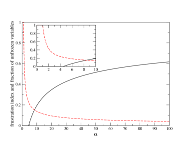
Figure 1: The long range frustration order parameter $R$ (solid lines) and the unfrozen probability $q_{0}$ (dashed lines) as a function of $\alpha$ for the random $2$-SAT problem. The inset is an amplification of the region of $\alpha\in[0,10]$.

The unfrozen probability $q_{0}$ and the long range frustration order parameter $R$, as calculated by Eqs. (7) and (9), are shown in Fig. 1 as a function of the clauses-to-variables ratio $\alpha$. Onset of spin freeze occurs at $\alpha=\alpha_{c}(2)=1$. This point, as shown later, is also the point of SAT–UNSAT transition, in agreement with the rigorous mathematical proof Fernandez de la Vega (2001). A typical random $2$-SAT formula of $\alpha<1$ is satisfiable while a typical random $2$-SAT formula of $\alpha>1$ is unsatisfiable. However, onset of long range frustration is delayed to $\alpha=\alpha_{R}(2)=4.4588$. For $\alpha_{c}(2)<\alpha<\alpha_{R}(2)$ a typical random $2$-SAT formula, although being unsatisfiable, is not long–range frustrated. We know that to determine the satisfiability of a $2$-SAT formula is computationally easy. It is interesting to point out that, long range frustration is absent at both sides of the SAT-UNSAT transition $\alpha_{c}(2)$ for the random $2$-SAT problem.

Based on our calculation that a randomly constructed $2$-SAT formula in the parameter regime of $\alpha_{c}(2)<\alpha<\alpha_{R}(2)$ is not long–range frustrated ($R=0$), we hope that a Boolean assignment that satisfies the largest possible number of its clauses might be easily found in practice, despite the fact that the MAX-$2$-SAT problem is in general NP-hard Fernandez de la Vega (2001). We will check this point by computer simulations in a later work.

When $\alpha\geq\alpha_{R}(2)$, long range frustrations exist among a fraction of the unfrozen variable nodes. Interestingly, the point $\alpha=\alpha_{R}(2)$ also marks the beginning of divergence of the population dynamics of the next subsection.

Now we turn to the ground–state energy density $\epsilon$. The energy increase $\epsilon_{1}$ due to the addition of variable node $i$ is

$$\epsilon_{1}(\alpha)=\sum\limits_{m_{+}=0}^{\infty}\sum\limits_{m_{-}=0}^{\infty}P_{\rm v}(m_{+})\ P_{\rm v}(m_{-})\ \min(m_{+},m_{-})\ .$$ (10)

After the addition of variable node $i$, the factor graph $G^{\prime}$ has $N+1$ variable nodes and on average $\alpha N+K\alpha$ function nodes ($K=2$). Its clauses-to-variables ratio is therefore $\alpha^{\prime}=\alpha+(K-1)\alpha/(N+1)$. Suppose the energy density $\epsilon$ of the system is a function only of $\alpha$. Then from the identity

$$(N+1)\epsilon(\alpha^{\prime})=N\epsilon(\alpha)+\epsilon_{1}\ ,$$

we obtain the following differential equation

$$\epsilon(\alpha)+(K-1)\alpha{{\rm d}\epsilon\over{\rm d}\alpha}=\epsilon_{1}$$

in the limit of large $N$. By solving this differential equation, we obtain that

$$\epsilon(\alpha)={1\over(K-1)\alpha^{1/(K-1)}}\int_{0}^{\alpha}\tilde{\alpha}^{{2-K\over K-1}}\epsilon_{1}(\tilde{\alpha}){\rm d}\tilde{\alpha}\ ,$$ (11)

where $K=2$. According to the author’s unpublished calculations, in the vertex cover problem, the energy density derived through this way is the exact ground–state energy density when there is no long range frustration; however, when $R>0$, this energy density is lower than the actual ground–state energy density obtained by Weigt and Hartmann by numerical means Weigt and Hartmann (2000) (the reason, however, is still unknown). We expect the same situation will occur here in the random $K$-SAT problem.

When long range frustration exists ($R>0$), an upper bound for the ground–state energy density $\epsilon$ can also be derived. For the enlarged factor graph $G^{\prime}$ to have clauses-to-variables ratio $\alpha$, on average $(K-1)\alpha$ function nodes must be removed Mézard and Parisi (2003). The energetic contribution of these function nodes must also be removed. This contribution comes from two parts: (i) the energy sum of these individual function nodes, $\Delta E=(K-1)\alpha[(1-q_{0})/2]^{K}$ and, (ii) additional energy $\Delta E^{\prime}$ caused by possible long range frustration among these function nodes. Therefore,

$$\epsilon(\alpha)=\epsilon_{1}-\Delta E-\Delta E^{\prime}.$$ (12)

If we set $\Delta E^{\prime}=0$, Eq. (12) then gives an upper bound.

The energy densities calculated based on Eqs. (11) and (12) are shown in Fig. 2. When $\alpha>\alpha_{c}(2)$, the energy density becomes positive and the system is UNSAT. In the range of $\alpha_{c}(2)\leq\alpha<\alpha_{R}(2)$, both Eq. (11) and (12) give the identical results, indicating that when there is no long range frustration, these equations are exact. When $\alpha\geq\alpha_{R}(2)$, the energy density given by Eq. (12) is systematically higher than that given by Eq. (11). In this regime of long range frustration, at the moment the author is still unable to give an exact ground–state energy density expression. We hope to return to this point in a future work.

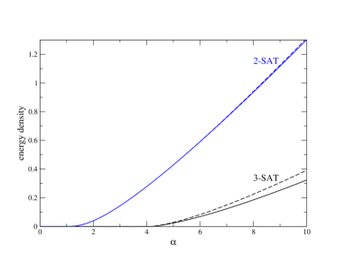
Figure 2: The energy density lower bound (solid lines) and upper bound (dashed lines) for the random $2$-SAT and $3$-SAT problem as a function of $\alpha$.

III.2 Random $2$-satisfiability studied by population dynamics

In this subsection, we study the random $2$-SAT problem following the zero–temperature cavity method treatment of Ref. Mézard and Zecchina (2002). Since in the parameter range of $0\leq\alpha<\alpha_{R}(2)$ there is no long range frustration, we expect this treatment to be exact in this range.

Suppose there are many macroscopic states of global minimum energy. Let us randomly choose a function node $a$ and follow one of its edges to a variable node $i$. Before the edge $(a,i)$ is connected, variable node $i$ may be positively frozen in some macroscopic states, and be negatively frozen in some other macroscopic states, and be unfrozen in the remaining macroscopic states. A positively (negatively) frozen variable node is said to feel a positive (negative) cavity field $h_{i}$, while an unfrozen variable node is said to feel a zero cavity field $h_{i}$ Mézard and Parisi (2003). The (modified) cavity field $J_{a}^{i}h_{i}$ distribution among all the macroscopic states (referred to as the cavity field survey) is denoted by $P(J_{a}^{i}h_{i})$, where $J_{a}^{i}$ is the bond strength between function node $a$ and variable node $i$. Besides function node $a$, node $i$ is connected by positive bonds to $p$ other function nodes $b_{1},\ldots,b_{p}$ and by negative bonds to $n$ other function nodes $c_{1},\ldots,c_{n}$.

Assuming there is no long range frustration among the unfrozen variable nodes ($R=0$), one can write down the following self-consistent equation for the cavity field distribution $P(J_{a}^{i}h_{i})$ Braunstein et al. (2002):

$$P(J_{a}^{i}h_{i}) \propto \int\bigl{[}\prod\limits_{r=1}^{p}P(J_{b_{r}}^{j_{r}}h_{j_{r}}){\rm d}h_{j_{r}}\bigr{]}\bigl{[}\prod\limits_{l=1}^{n}P(J_{c_{l}}^{k_{l}}h_{k_{l}}){\rm d}h_{k_{l}}\bigr{]}\times$$ (13)

$$\delta\bigl{(}J_{a}^{i}h_{i}-\sum\limits_{r=1}^{p}\theta(-J_{b_{r}}^{j_{r}}h_{j_{r}}\bigr{)}+\sum\limits_{l=1}^{n}\theta(-J_{c_{l}}^{k_{l}}h_{k_{l}}))\times$$

$$\exp(-y\Delta E_{1}/2)$$

where $\theta(x)$ is the Heaviside step function, $\theta(x)=1$ if $x>0$ and $\theta(x)=0$ otherwise; $y$ is a re-weighting parameter; and

$$\Delta E_{1} = \sum_{r=1}^{p}\theta(-J_{a_{r}}^{j_{r}}h_{j_{r}})+\sum_{l=1}^{n}\theta(-J_{b_{l}}^{k_{l}}h_{k_{l}})$$ (14)

$$-|\sum_{r=1}^{p}\theta(-J_{a_{r}}^{j_{r}}h_{j_{r}})-\sum_{l=1}^{n}\theta(-J_{b_{l}}^{k_{l}}h_{k_{l}})|$$

is twice the energy caused by the function nodes $b_{1},\ldots,b_{p},c_{1},\ldots,c_{n}$.

In the limit of $y\to+\infty$, the general form of the cavity field distribution is Braunstein et al. (2002)

$$P(J_{a}^{i}h_{i})=\left\{\begin{array}[]{ll}P_{+}(J_{a}^{i}h_{i})\ ,&p_{+}\\ P_{-}(J_{a}^{i}h_{i})\ ,&p_{-}\\ \begin{array}[]{r}\eta_{0}(i)\delta(J_{a}^{i}h_{i})+\eta_{+}(i)P_{+}(J_{a}^{i}h_{i})\\ +\eta_{-}(i)P_{-}(J_{a}^{i}h_{i})\ .\end{array}&p_{0}\end{array}\right.$$ (15)

In Eq. (15), $p_{+}$, $p_{-}$, and $p_{0}$ are the probabilities of occurrence for the three types of cavity field surveys. $P_{+}(k)$ is a probability distribution over positive integers $k$; and $P_{-}(k)$ is a probability distribution over negative integers $k$. The parameters $\eta_{0}(i)$, $\eta_{+}(i)$, and $\eta_{-}(i)$ are three random variables, $\eta_{0}(i)+\eta_{+}(i)+\eta_{-}(i)=1$.

Based on Eqs. (13) and (15), one finds that

$$p_{0}=\sum\limits_{m=0}^{\infty}{e^{-\alpha(1-p_{0})}\bigl{(}\alpha(1-p_{0})/2\bigr{)}^{2m}\over(m!)^{2}}\ ,$$ (16)

$$p_{+}=p_{-}=(1-p_{0})/2\ .$$ (17)

When $\alpha\leq\alpha_{R}(2)$, the probability $p_{0}$ satisfies $\alpha p_{0}\leq 1$. Consequently, the population dynamics at $y=\infty$ converges to the replica symmetric fix point of $\eta_{0}\equiv 1,\eta_{+}=\eta_{-}\equiv 0$. In other words, the system has only one macroscopic state. When $\alpha>\alpha_{R}(2)$, this replica symmetric fixed point is unstable, and if initially the random variables $\eta_{0}(i)$ are slightly less than unity, the population dynamics at $y=\infty$ becomes divergent. This divergence suggests that, at this parameter regime, the assumption of absence of long range frustration becomes invalid.

To get rid of this divergence, one can run population dynamics at a finite positive value of $y$. A conceptually better way is to directly take into account the effect of long range frustration in the population dynamics. Unfortunately, at the moment the author is unable to achieve this goal.

III.3 The $\pm J$ Viana–Bray spin glass model

We now briefly discuss the zero temperature phase diagram of the $\pm J$ Viana–Bray model Viana and Bray (1985). The model is characterized by the Hamiltonian

$$E[\{\sigma_{i}\}]=-\sum\limits_{(ij)}J_{ij}\sigma_{i}\sigma_{j}\ ,$$ (18)

where the summation is over all the edges $(ij)$ of a Poisson random graph of mean vertex degree $c$; the edge strength $J_{ij}=\pm 1$, with equal probability; and $\sigma_{i}=\pm 1$ is the spin value on vertex $i$. The zero temperature phase diagram of this model was first reported in Ref. Kanter and Sompolinsky (1987) through the replica approach. It was found that, when $c\leq 1$, the system is in the paramagnetic phase with no frozen vertices, i.e., $q_{0}=1$; when $c>1$, the system is in the spin glass phase, where some vertices are frozen to positive or negative spin values, and $q_{0}$ gradually decreases from unity.

The Hamiltonian Eq. (18) is similar to that of the random $2$-SAT and can be studied by the same method mentioned in subsection III.1. We find that the zero temperature phase diagram of model (18) is identical to Fig. 1 of the random $2$-SAT. The transition between the paramagnetic phase and the spin glass phase occurs at $c=1$, confirming the earlier result of Ref. Kanter and Sompolinsky (1987). (When the long range frustration order parameter is set to $R=0$, the order parameter $q_{0}$ has the same expression as Eq. (15) of Ref. Kanter and Sompolinsky (1987).) In the spin glass phase, long range frustration among unfrozen vertices only builds up ($R>0$) when the mean vertex degree $c\geq 4.4588$.

The $\pm J$ finite connectivity spin glass model therefore has two types of phase transitions as the mean connectivity is increased. First there is the frozen transition to the spin glass phase; and then there is the transition to a long–range frustrated spin glass phase. It is more experimentally relevant to discuss the phase transitions in terms of temperature. It is accepted that the spin glass phase will persist over a finite temperature range of $0\leq T<T_{g}$ Viana and Bray (1985). We expect that when the mean vertex degree $c>4.4588$, the long–range frustrated spin glass phase will also persist over a temperature range of $0\leq T<T_{R}$, with $T_{R}\leq T_{g}$. It will be of great interest to check the validity of this picture by computer simulations.

Real world spin glass materials are three–dimensional, and their spin–spin interactions may be more complex than that given by Eq. (18). It is not known whether or not long range frustrations exist among the unfrozen vertices of such systems, and if they do exist, how to detect them experimentally. It may be useful to re-interprete the already documented experimental observations in terms of the long range frustration order parameter $R$.

IV The random $3$-satisfiability problem

This section focuses on the random $3$-SAT problem. We study it using the method of Sec. III.1 and then compare the results with those obtained by population dynamics.

The probability of a randomly chosen variable node being positively frozen, negatively frozen, or unfrozen in a macroscopic state $\beta$ of global minimum energy is denoted respectively as $q_{+}$, $q_{-}$, and $q_{0}$ as in the case of the random $2$-SAT problem. $R$ is the probability that an unfrozen variable node is type-I unfrozen with respect to a prescribed spin value. The parameters $q_{0}$, $q_{+}$, $q_{-}$, and $R$ can be obtained following the same procedure as was outlined in Sec. III.1. We first generate a factor graph $G$ of $N$ variable nodes and $M=\alpha N$ function nodes; we then create a new variable node $i$ and connect this new node $i$ to $G$ through the formation of $k$ new function nodes, with $k$ following the Poisson distribution $f(k,3\alpha)$. The other ends of such a function node $a$ are connected to two randomly chosen variable nodes $j$ and $k$ of the factor graph $G$. For convenience of discussion, we denote $\sigma_{j}^{*}=J_{a}^{j}$ and $\sigma_{k}^{*}=J_{a}^{k}$; and in the remaining part of this section, when we mention that a variable node $j$ is type-I or type-II unfrozen, we mean that it is type-I or type-II unfrozen with respect to the spin value $\sigma_{j}^{*}$. In state $\beta$, the function node $a$ faces one of the following local environments:

(i).

Node $j$ is frozen in factor graph $G$ to $\sigma_{j}\equiv\sigma_{j}^{*}$ or node $k$ is frozen to $\sigma_{k}=\sigma_{k}^{*}$. This happens with probability $(3-2q_{0}-q_{0}^{2})/4$. In this situation, function node $a$ is satisfied by $j$ or $k$ (or both).

(ii).

Both node $j$ and node $k$ are type-II unfrozen. This happens with probability $q_{0}^{2}(1-R)^{2}$. In this situation, function node $a$ is satisfiable by $j$ and $k$.

(iii).

One of the two variable nodes, say $j$, is type-II unfrozen while the other, $k$, is type-I unfrozen. This happens with probability $2q_{0}^{2}R(1-R)$. In this situation, node $a$ is satisfiable by $j$. (It is also satisfiable by node $k$ through setting $\sigma_{k}=\sigma_{k}^{*}$, but this spin flipping will perturb the spin values of $O(N)$ other unfrozen variable nodes.)

(iv).

Both node $j$ and node $k$ are type-I unfrozen, but they can not take the spin value $\sigma_{j}=\sigma_{j}^{*}$ and $\sigma_{k}=\sigma_{k}^{*}$ simultaneously in state $\beta$. This happens with probability $q_{0}^{2}R^{2}/2$. In this situation, node $a$ is definitely satisfied by one of nodes $j$ and $k$ (in some configurations of $\beta$, node $j$ satisfies $a$ while $\sigma_{k}=-\sigma_{k}^{*}$, and in the remaining configurations node $k$ satisfies $a$ while $\sigma_{j}=-\sigma_{j}^{*}$).

(v)

Both node $j$ and node $k$ are type-I unfrozen and they can take the spin value $\sigma_{j}=\sigma_{j}^{*}$ and $\sigma_{k}=\sigma_{k}^{*}$ simultaneously. This happens with probability $q_{0}^{2}R^{2}/2$. In this situation, node $a$ is also satisfiable by $j$ and $k$. However, to satisfy $a$ by node $j$ or $k$ will cause an extensive perturbation to the spin configuration, whereby the spin values of $O(N)$ other unfrozen variable nodes will eventually be fixed.

(vi).

One of the variable nodes, say $j$, is type-I unfrozen while the other is frozen to $\sigma_{k}=-\sigma_{k}^{*}$. This happens with probability $2q_{0}q_{-}R$. In this situation, node $a$ is satisfiable by node $j$, with the same consequence as in situation (v).

(vii).

One of the variable nodes, say $j$, is type-II unfrozen while the other is frozen to $\sigma_{k}=-\sigma_{k}^{*}$. This happens with probability $2q_{0}q_{-}(1-R)$. In this situation, node $a$ is satisfiable by node $j$.

(viii).

Node $j$ is frozen to $\sigma_{j}=-\sigma_{j}^{*}$ and node $k$ is frozen to $\sigma_{k}=-\sigma_{k}^{*}$. This happens with probability $q_{-}^{2}$. In this situation, node $a$ is satisfiable only if the spin value of variable node $i$ is set to $\sigma_{i}=J_{a}^{i}$.

For the random $3$-SAT problem, the parameter $q_{0}$ is also determined self-consistently by Eq. (7), with the only difference that $\lambda_{1}=(3/2)\alpha[q_{0}^{2}R^{2}/2+2q_{0}q_{-}R]$ and $\lambda_{2}=(3/2)\alpha q_{-}^{2}$; and the parameter $R$ is determined by Eq. (9), with $\lambda_{3}=3\alpha q_{0}q_{-}(1-R)$. The lower and upper bound of the global minimum energy density can be obtained through Eqs. (11) and (12), with $K=3$. The values of the long range frustration order parameter $R$ and the fraction of unfrozen variable nodes $q_{0}$ are shown in Fig. 3 as a function of $\alpha$, and the energy density lower and upper bounds are shown in Fig. 2.

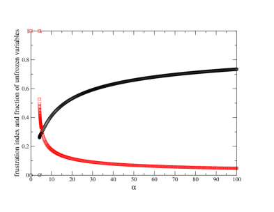
Figure 3: Long range frustration index $R$ (circles) and fraction of unfrozen variables $q_{0}$ (squares) as a function of clause-to-variable ratio $\alpha$ for the random $3$-SAT problem.

When $\alpha<\alpha_{R}(3)=4.189724$, Eqs. (7) and (9) permit only a trivial solution of $q_{0}\equiv 1$ and $R\equiv 0$, with zero energy density. When $\alpha\geq\alpha_{R}(3)$, this non-frustrated replica symmetric solution is still locally stable. However, at this parameter range, another stable self-consistent solution appears. This nontrivial solution is long–range frustrated, with its order parameter $R$ jumps from zero to $R=0.2605$ at $\alpha=\alpha_{R}(3)$, accompanied by a drop of $q_{0}$ from $q_{0}=1$ to $q_{0}=0.5270$. Interestingly, although there are jumps for the order parameters $R$ and $q_{0}$ at $\alpha_{R}(3)$, the energy density of this solution increases only gradually from zero as a function of $\alpha$ (see Fig. 2). This is an improvement over a previous mean field solution. If long range frustration was not taken into account, Eq. (7) predicts a nontrivial solution when $\alpha\geq 4.667$, which, however, has an unphysical negative energy density as long as $\alpha<5.18$ Monasson and Zecchina (1996, 1997).

The present mean field solution predicts that, in the parameter range of $\alpha\geq\alpha_{R}(3)$ a random $3$-SAT formula will be long–range frustrated and unsatisfiable. This predicted SAT-UNSAT transition point is located between the rigorously known lower and upper bounds Achlioptas (2001). However, through the zero temperature cavity method and population dynamics, it is found in Ref. Mézard and Zecchina (2002) that, when $3.921<\alpha<4.267$ the random $3$-SAT problem has another non-frustrated replica symmetry breaking solution with zero energy and positive structural entropy. The structural entropy of this non-frustrated solution becomes negative when $\alpha\geq 4.267$, and this point is regarded as the SAT-UNSAT transition point of the random $3$-SAT problem. Therefore, there is a clear discrepancy between the present work and the result of Ref. Mézard and Zecchina (2002). Two reasons are conceivable for this discrepancy:

First, the treatment in this paper is essentially replica symmetric, with only two order parameters $q_{0}$ and $R$. In the random $3$-SAT problem, it is clear that replica symmetry breaking occurs before the onset of long range frustration. This is different from what happens in the random $2$-SAT problem of Sec. III and the vertex cover problem of Ref. Zhou (2004). In those two systems, replica symmetry breaking occurs concomitantly with the onset of long range frustration. When replica symmetry is broken and there are many (macroscopic) states of global minimum energy, first, one needs more order parameters to characterize the system in the non-frustrated phase; and second, in the long–range frustrated phase, the group of type-I unfrozen variable nodes of one state as well as their spin value correlations may be quite different from those of another state. These two points make calculation quite difficult. It is hoped that the present work will stimulate future efforts on this line.

Second, the long–range frustrated mean field solution does not evolve from the instability of the non-frustrated solution. This is clear from the fact that, at $\alpha=\alpha_{R}(3)$, the long range frustration order parameter jumps to a positive value rather than gradually increases from zero. This is qualitatively different from what happens in the random $2$-SAT and the vertex cover problem, where long range frustration is caused by a propagation and percolation of frustration. Maybe the present frustrated solution correspond to a metastable macroscopic state rather than a state of global minimum energy. We believe that long range frustration will also exist in the ground–states of the random $3$-SAT problem when $\alpha$ is larger than some threshold value. If this onset of long range frustration is caused be a percolation of frustration as assumed in this paper, the order parameter $R$ should gradually increases from zero.

The author has also performed a stability analysis of the replica symmetry breaking solution of Ref. Mézard and Zecchina (2002), to investigate whether or not long range frustration will occur gradually when $\alpha\geq 4.267$. His preliminary simulation results indicate that this solution is also locally stable at $\alpha\sim 4.267$.

V Conclusion and discussion

In a random $K$-SAT problem, some of the variable nodes are unfrozen, their spin values change in different microscopic configurations of global minimum energy. However, these fluctuations of spin values among different unfrozen variable nodes may be highly correlated. In this paper, we have investigated the possibility of such kind of correlations based on the physical picture of percolation transition. For the random $2$-SAT problem, we found that long range frustration among unfrozen variable nodes gradually builds up as the clauses-to-variables ratio $\alpha$ exceeds $\alpha_{R}(2)=4.4588$. This value is larger than the SAT-UNSAT transition point of $\alpha_{c}(2)=1$. For the random $3$-SAT problem, we found a long–range frustrated mean field solution when $\alpha>\alpha_{R}(3)=4.1897$. The energy density of this solution increases gradually from zero as a function of $\alpha$, while there is a jump in the long range frustration order parameter $R$ at $\alpha_{R}(3)$. The SAT-UNSAT transition point of this nontrivial solution is lower than the value of $\alpha_{c}(3)=4.267$ as predicted by the work of Refs. Mézard et al. (2002); Mézard and Zecchina (2002); Braunstein et al. (2002). Two possible reasons for this discrepancy were mentioned. This discrepancy indicates that, when replica symmetry breaking occurs before the onset of long range frustration, the present mean field theory needs to be improved. We hope the present work will stimulate further efforts to overcome this difficulty.

The phase diagram of the finite connectivity $\pm J$ Viana–Bray spin glass model was also discussed. We suggested the possibility of a phase transition from a non-frustrated spin glass phase to a long–range frustrated spin glass phase as a finite temperature. This prediction might be checked by numerical simulations.

The method used in the present work may also be applicable to other finite connectivity spin glass models Viana and Bray (1985). We hope that an appropriate combination of long range frustration and the cavity method at the first order replica symmetry breaking level Mézard and Parisi (2001, 2003) will help to advance our understanding of spin glass statistical physics.

There exists a rigorously polynomial algorithm to solve the $2$-SAT decision problem; but the $3$-SAT decision problem is NP-complete. The proliferation of macroscopic domains in the solution spaces of the $3$-SAT problem and its absence in the $2$-SAT problem is unlikely to be the reason for this qualitative difference in computational complexity, since there exist class P (polynomial) combinatorial optimization problems which also have exponentially many macroscopic states in their solution spaces Mézard et al. (2003); Zhou and Ou-Yang (2003). In the author’s opinion, an instance of a combinatorial optimization problem may become intrinsically difficult if long range frustration of the type discussed in this paper exists in such a system. Long range frustration causes strong correlations among the fluctuations of the spin values of a finite fraction of the vertices of the system. This means that, if the spin on an unfrozen vertex is set to a given value, the spins on other $O(N)$ unfrozen vertices should also be set to the corresponding values. This spin value fixation process may be extremely difficult to achieve even for a global algorithm, since the algorithm needs to choose the right vertices and the right spin values to fix.

In the random $2$-SAT problem, there is no long range frustration at both sides of the SAT-UNSAT transition point. In the vertex cover problem, there is an onset of long range frustration in the computationally difficult case of mean vertex degree $c\geq 2.7183$ Zhou (2004). In the random $3$-SAT problem, we know there exists a non-trivial solution with a jump of the long range frustration order parameter $R$ at $\alpha_{R}(3)$. Although $\alpha_{R}(3)$ is unlikely to be true SAT-UNSAT phase transition point for this problem, we expect to observe that, in a correct replica symmetry breaking mean field solution long range frustration will builds up when the clauses-to-variables ratio $\alpha\geq\alpha_{c}(3)$. To construct such a mean field solution is still an open problem.

References

- Zhou (2004) H. Zhou, Long range frustration in a spin glass model of the vertex cover problem, e-print: cond-mat/0411077 (2004) [Phys. Rev. Lett. 94 (2005)].
- Garey and Johnson (1979) M. Garey and D. S. Johnson, Computers and Intractability: A Guide to the Theory of NP-Completeness (Freeman, San Francisco, 1979).
- Aspvall et al. (1979) B. Aspvall, M. F. Plass, and R. E. Tarjan, Inf. Process. Lett. 8, 121 (1979).
- Cheeseman et al. (1991) P. Cheeseman, B. Kanefsky, and W. Taylor, in Proc. 12th Int. Conf. on Artif. Intelligence, edited by R. Reiter and J. Mylopoulos (Morgan Kaufmann, San Mateo, CA, 1991), pp. 331–337.
- Kirkpatrick and Selman (1994) S. Kirkpatrick and B. Selman, Science 264, 1297 (1994).
- Crawford and Auton (1996) J. M. Crawford and L. D. Auton, Artif. Intell. 81, 31 (1996).
- Achlioptas (2001) D. Achlioptas, Theor. Comput. Sci. 265, 159 (2001).
- Monasson and Zecchina (1996) R. Monasson and R. Zecchina, Phys. Rev. Lett. 76, 3881 (1996).
- Monasson and Zecchina (1997) R. Monasson and R. Zecchina, Phys. Rev. E 56, 1357 (1997).
- Monasson et al. (1999) R. Monasson, R. Zecchina, S. Kirkpatrick, B. Selman, and L. Troyansky, Nature 400, 133 (1999).
- Mézard et al. (2002) M. Mézard, G. Parisi, and R. Zecchina, Science 297, 812 (2002).
- Mézard and Zecchina (2002) M. Mézard and R. Zecchina, Phys. Rev. E 66, 056126 (2002).
- Braunstein et al. (2002) A. Braunstein, M. Mézard, and R. Zecchina, Survey propagation: an algorithm for satisfiability, e-print: cs.CC/0212002 (2002).
- Mézard and Parisi (2003) M. Mézard and G. Parisi, J. Stat. Phys. 111, 1 (2003).
- Mézard and Parisi (2001) M. Mézard and G. Parisi, Eur. Phys. J. B 20, 217 (2001).
- Bollobás (1985) B. Bollobás, Random Graphs (Academic Press, Landon, 1985).
- Fernandez de la Vega (2001) W. Fernandez de la Vega, Theor. Comput. Sci. 265, 131 (2001).
- Weigt and Hartmann (2000) M. Weigt and A. K. Hartmann, Phys. Rev. Lett. 84, 6118 (2000).
- Viana and Bray (1985) L. Viana and A. J. Bray, J. Phys. C: Solid State Phys. 18, 3037 (1985).
- Kanter and Sompolinsky (1987) I. Kanter and H. Sompolinsky, Phys. Rev. Lett. 58, 164 (1987).
- Mézard et al. (2003) M. Mézard, F. Ricci-Tersenghi, and R. Zecchina, J. Stat. Phys. 111, 505 (2003).
- Zhou and Ou-Yang (2003) H. Zhou and Z.-C. Ou-Yang, Maximum matching on random graphs, e-print: cond-mat/0309348 (2003).