Critical scaling of thermal transport in model A dynamics for a superconductor

Abstract

We consider the scaling of thermal transport in the presence of electric and magnetic fields near the finite temperature transition from the metallic normal state to the superconductor. We do so with fully relaxational, model A, dynamics for the order parameter and particle-hole symmetry. This enables us to determine the exact scaling dimension of the heat current operator and hence critical exponents for all transport coefficients in terms of the (approximately) known values of the correlation length exponent and the dynamic scaling exponent. In particular, we determine the critical behavior for the Nernst coefficient.

I Introduction

The discovery of high-temperature superconductors has led to a renewed interest in superconducting fluctuations. In these materials, the effect of fluctuations may be strong, with a relatively large critical regime, due to their short coherence lengths, quasi-two-dimensionality and high transition temperatures Fisher-Fisher-Huse . Neglecting fluctuations of the gauge potential, the transition to the superconducting state is described by a complex order parameter and is of the XY universality class (in three dimensions, due to interlayer coupling). This description holds well in strongly type-II superconductors except extremely close to the critical temperature $T_{c}$ where one crosses over to the critical behavior of a charged superconductor invertedXY . The description of dynamic properties, such as transport, requires coupling this thermodynamic description to a dynamic equation, which for superconductors is usually assumed to be model A in the classification of Hohenberg and Halperin Hohenberg-Halperin .

Of particular interest in this context are the recent measurements of the Nernst coefficient in the cuprates Ong . The large Nernst signal observed in these experiments above $T_{c}$ is likely the contribution of superconducting fluctuations. This interpretation provides a quantitative agreement with experiment in overdoped samples in the regime where a Gaussian approximation is applicable Ussishkin-Sondhi-Huse , as well as in the vortex liquid regime Mukerjee . In underdoped samples it requires a stronger effect of fluctuations, which would have important implications for the physics of the pseudogap regime Ussishkin-Sondhi .

In this paper, we focus our attention on the scaling behavior of thermal transport in the XY critical regime. The transport coefficient of interest for the Nernst effect is the transverse thermoelectric response $\alpha_{xy}$ alpha-xy . For this, we consider the scaling of the heat current operator, which also allows us to treat the thermal conductivity on the same footing. As with the conductivity Fisher-Fisher-Huse ; Wickham-Dorsey , it is necessary to specify the dynamics associated with the order parameter for analyzing thermal transport. We then find the scaling dimension of the heat current operator, and obtain general scaling forms for thermal transport. The critical behavior of both the thermal and thermoelectric transport coefficients is then deduced.

We follow the usual assumption for a superconductor, and consider relaxational dynamics for a non-conserved order parameter, or model A dynamics Hohenberg-Halperin ; fn-model . We further assume that the model is particle-hole symmetric which allows much progress to be made. When needed, the order parameter may be coupled to an electromagnetic field, whose dynamics we ignore, keeping our calculation in the XY regime Lennart .

The main result of this paper is simply stated: the heat current operator in model A,

$$\mathbf{j}^{Q}=-\frac{\partial\psi^{*}}{\partial t}\nabla\psi+\text{c.c.},$$ (1)

does not acquire an anomalous dimension. This result is surprising on two counts: First, the heat current is not a conserved quantity in model A and second, the scaling dimension of the heat current does not involve the dynamic critical exponent $z$, despite its dynamic nature. Technically we will find that there is a “hidden” conservation law at play in the model. We note that a similar absence of an anomalous dimension is well known for the electric current Fisher-Fisher-Huse ,

$$\mathbf{j}\propto-i\psi^{*}\nabla\psi+\text{c.c.}.$$ (2)

In this case, however, there are conserved (solenoidal) supercurrents in the purely static theory and thus the result is less mysterious.

With this result, critical exponents of various thermal transport coefficients may now be deduced. In particular, we find that to linear order in magnetic field, the transverse thermoelectric response $\alpha_{xy}$ scales in three dimensions as $\alpha_{xy}/B\propto\xi^{z-1}$, where $\xi$ is the (temperature-dependent) correlation length of the superconductor. Whether this prediction may be observable in the critical 3D-XY regime of cuprates remains to be seen.

Below we present our calculations in detail: After defining the model in Sec. II, we obtain the anomalous dimension of the heat current operator (or rather, its absence thereof) in Sec. III. We briefly address the problem of introducing a temperature gradient in Sec. IV. The scaling relations for thermal transport and their consequences are discussed in Sec. V, which is followed by a brief summary.

II Model A

In this paper, we consider model A dynamics for a complex superconducting order parameter. The order parameter dynamics in this model is given by the stochastic equation

$$\frac{\partial\psi}{\partial t}=-\Gamma_{0}\frac{\delta F}{\delta\psi^{*}}+\zeta,$$ (3)

with the Landau-Ginzburg-Wilson free energy

$$F=\int d\mathbf{x}\left(r_{0}|\psi|^{2}+u_{0}|\psi|^{4}+|\nabla\psi|^{2}\right).$$ (4)

In Eq. (3), $\Gamma_{0}$ is the relaxation rate for the order parameter, which we assume in this paper to be real (making the model particle-hole symmetric). Thermal fluctuations are introduced with $\zeta$, which is a Gaussian white noise with correlator

$$\langle\zeta^{*}(\mathbf{x},t)\zeta(\mathbf{x^{\prime}},t^{\prime})\rangle=2\Gamma_{0}T\delta(\mathbf{x}-\mathbf{x^{\prime}})\delta(t-t^{\prime}).$$ (5)

Unlike the usual convention in critical dynamics, we have explicitly expressed the temperature $T$, which will be useful below. The correlation function of the noise ensures that the probability that an order parameter configuration $\psi$ will occur is $P\{\psi\}=Z^{-1}\exp[-F\{\psi\}/T]$ (where $Z=\int D\{\psi\}\exp[-F\{\psi\}/T])$.

The main object we consider within this model is the operator of heat current (1). This form may be understood in terms of the transport of free energy. In Sec. IV we note how it arises from considerations involving the application of a temperature gradient to the system. It also arises in derivations of time-dependent Ginzburg-Landau equations from microscopics. Note that the heat current operator is a dynamic object involving a time derivative (unlike the electric current); thus its properties are dependent on the choice of dynamics.

When particle-hole symmetry is broken, the relaxation rate $\Gamma_{0}$ becomes complex, and model A admits non-dissipative, or reactive, terms. While we expect such terms not to contribute to heat transport, the question of incorporating this expectation into the critical dynamics treatment of the heat current is not fully resolved. In this paper, we therefore proceed with the assumption particle-hole symmetry.

III Scaling dimension of $\mathbf{j}^{Q}$

In this section, we consider the scaling dimension $d_{Q}$ of the heat current operator. The dimension $d_{Q}$ will then allow us to write scaling forms for properties involving the heat current, as we do in Sec. V for thermal and thermoelectric transport. Naively, one may expect the emergence of an anomalous dimension for this operator (i.e., a deviation from its Gaussian value). In particular, because of the explicit time derivative in $\mathbf{j}^{Q}$ [Eq. (1)], one may expect the anomalous dimension to involve the dynamical critical exponent $z$. In this section we show that these expectations are false; we find $d_{Q}=d+1$ in $d$ dimensions, with no anomalous dimension. We do so first by an exact argument, then by sketching the calculation of $d_{Q}$ to second order in an $\epsilon$ expansion.

We begin by replacing the dynamic stochastic equation with an effective action for calculating dynamic correlators Zinn-Justin . Consider the Langevin equation given by Eq. (3) (in this section we set $T=1$). The noise term has a Gaussian distribution,

$$P\{\zeta(x,t)\}\propto\exp\left(-\int d^{d}x\,dt\,\frac{|\zeta(x,t)|^{2}}{2\Gamma_{0}}\right).$$ (6)

Enforcing Eq. (3) by a $\delta$ function, expectation values, when averaged over the noise distribution, take the form

$$\langle\cdots\rangle_{\zeta}\propto\int D\psi\,D\zeta\,\cdots\,\delta\left(\frac{\partial\psi}{\partial t}+\Gamma_{0}\frac{\delta F}{\delta\psi^{*}}-\zeta\right)P\{\zeta(x,t)\}.$$ (7)

The integral over the noise may now be performed, yielding an effective action for $\psi$,

$$\langle\cdots\rangle\propto\int D\psi\,\cdots\,e^{-S_{\text{eff}}\{\psi\}},$$ (8)

where

$$S_{\text{eff}}\{\psi\} = \frac{1}{2\Gamma_{0}}\int d^{d}x\,dt\,\left|\frac{\partial\psi}{\partial t}+\Gamma_{0}\frac{\delta F}{\delta\psi^{*}}\right|^{2}$$

$$= \frac{1}{2\Gamma_{0}}\int d^{d}x\,dt\,\left|\frac{\partial\psi}{\partial t}\right|^{2}+\left|\Gamma_{0}\frac{\delta F}{\delta\psi^{*}}\right|^{2}.$$

The last step uses the fact that the cross term in the action is a full derivative and hence vanishes upon integration. In the above, we have ignored the Jacobian term, which is irrelevant for the renormalization group analysis Zinn-Justin . The problem of calculating dynamical correlation function is thus expressed in terms of a new effective action $S_{\text{eff}}$, which may be viewed either as a quantum mechanical action (the view adopted here), or equivalently as a classical statistical mechanical action in $d+1$ dimensions.

The exact argument regarding the dimension of the heat current operator is based on the following observation: The heat current, Eq. (1), is proportional to the conserved momentum density of the effective Lagrangian,

$$T_{0i}=\frac{\partial\mathcal{L}_{\text{eff}}}{\partial(\partial_{0}\psi)}\partial_{i}\psi+\text{c.c.}=\frac{1}{\Gamma_{0}}\left(\frac{\partial\psi^{*}}{\partial t}\nabla_{i}\psi+\text{c.c.}\right).$$ (10)

This observation essentially sets the dimension of the heat current operator; it does not have an anomalous dimension because it is conserved. A similar argument, but in the purely static theory, fixes the dimension of the electric current operator as $d_{e}=d-1$.

A standard argument turns the conservation law into a Ward identity. Consider a time-ordered correlation function of $T_{0i}$ with a set of operators $\psi$ (whose dimension is known),

$$\left\langle\mathcal{T}T^{\mu i}(x)\psi(x_{1})\ldots\psi(x_{n})\right\rangle.$$ (11)

(Here, we use $x$ to denote both $x$ and $t$ in the arguments of the fields.) Using $\partial^{\mu}T_{\mu i}=0$ (as $T_{\mu i}$ is a conserved current for each of its components $i$), we only need to account for the time-derivative on the step functions due to time-ordering,

$$\partial^{\mu}\left\langle\mathcal{T}T_{\mu i}(x)\psi(x_{1})\ldots\psi(x_{n})\right\rangle$$

$$=\sum_{j=1}^{n}\delta(t-t_{i})\langle\psi(x_{1})\ldots[T_{0i}(x),\psi(x_{j})]\ldots\psi(x_{n})\rangle$$

$$=-i\sum_{j=1}^{n}\delta^{(d+1)}(x-x_{i})\langle\psi(x_{1})\ldots\partial_{i}\psi(x_{j})\ldots\psi(x_{n})\rangle.$$

The dimension of the heat current operator, $d_{Q}=d+1$, may be deduced from Eq. (III) by comparing the term with $\mu=0$ in the first line (involving the required heat current operator) with the last line of the equation (where all the dimensionalities are known). The dimensionality of the fields $\psi(x_{i})$ cancel between the two sides, as does the factor $z$ between the time derivative in the first line and the time component of the $\delta$ function in the last line. The spatial part of the $\delta$ function and the additional spatial derivative in the last line give the dimension of the heat current operator.

As the result above is not very transparent in terms of its physical content it is instructive to see how this works in an expansion about the Gaussian fixed point; indeed, this is how we came across this result in the first place. Specifically we consider the expansion in $\epsilon=4-d$ to second order (the first non-trivial order) for the dimension of the heat current. We find that the coefficients of this expansion vanish, thus corroborating the exact argument above.

The calculation proceeds by adapting the method for computing dimensions of composite operators outlined by Wilson and Kogut Wilson-Kogut to the dynamic theory. For convenience, the complex order parameter $\psi$ is represented in this calculation in terms of its real and imaginary components, $\psi=\phi_{1}+i\phi_{2}$, and the heat current operator is then

$$\mathbf{j}^{Q}\propto-\frac{\partial\phi_{1}}{\partial t}\,\nabla\phi_{1}-\frac{\partial\phi_{2}}{\partial t}\,\nabla\phi_{2}.$$ (13)

We consider the following correlation function involving the heat current operator

$$\mathbf{U}(\mathbf{q},\omega)=\int d\mathbf{x}\,d\mathbf{x^{\prime}}\,dt\,dt^{\prime}e^{i\mathbf{q}\cdot(\mathbf{x}-\mathbf{x^{\prime}})-i\omega(t-t^{\prime})}$$

$$\qquad\qquad\qquad\qquad\times\,\left\langle\phi_{i}(\mathbf{x},t)\phi_{i}(\mathbf{x^{\prime}},t^{\prime})\mathbf{j}^{Q}(0,0)\right\rangle.$$

Following Wilson and Kogut, the correlation function has been chosen both for its simplicity and because it avoids the mixing in of operators involving total derivatives.

By simple counting of dimensions, the correlation function may be expressed (in terms of an unknown scaling function $\mathbf{F}$) as

$$\mathbf{U}=\xi^{2d+2z-2d_{s}-d_{Q}}\mathbf{F}(\mathbf{q}\xi,\omega\xi^{z}),$$ (15)

Here, $\xi$ is the correlation length, $d_{Q}$ is the unknown dimension of the heat current operator, and $d_{s}=(d-2+\eta)/2$ is the dimension of the operator $\phi_{i}$. This result may be expressed in terms of the $\langle\phi_{i}\phi_{i}\rangle$ static correlator at $\mathbf{q}=0$, $r^{-1}\propto\xi^{2-\eta}$. Expanding to linear order in $\mathbf{q}$ and $\omega$, we thus have

$$\mathbf{U}\propto\mathbf{q}\,\omega\,r^{(d_{Q}+\eta-d-3-3z)/(2-\eta)}.$$ (16)

This result will be compared with a perturbative calculation of $\mathbf{U}$ to obtain the result for $d_{Q}$.

We briefly outline the calculation of $\mathbf{U}$. The perturbative method for the dynamic case (see, e.g., Ref. Ma ) begins by presenting the fields as

$$\phi_{i}(\mathbf{k},\omega)=\phi_{i}^{(0)}(\mathbf{k},\omega)-uG_{0}(\mathbf{k},\omega)\sum_{j}\int\frac{d\mathbf{k^{\prime}}\,d\mathbf{k^{\prime\prime}}\,d\omega^{\prime}\,d\omega^{\prime\prime}}{(2\pi)^{2(d+1)}}$$ (17)

$$\!\!\!\!\!\!\!\times\,\phi_{j}(\mathbf{k^{\prime}},\omega^{\prime})\phi_{j}(\mathbf{k^{\prime\prime}},\omega^{\prime\prime})\phi_{i}(\mathbf{k}-\mathbf{k^{\prime}}-\mathbf{k^{\prime\prime}},\omega-\omega^{\prime}-\omega^{\prime\prime}).\qquad\;$$

Here, $\phi_{i}^{(0)}=G_{0}(\mathbf{k},\omega)\zeta_{i}(\mathbf{k},\omega)/\Gamma$ is the free field, and

$$G_{0}(\mathbf{k},\omega)=\frac{1}{r+k^{2}-i\omega/\Gamma}$$ (18)

is the free propagator. Equation (17) is then used to generate the different diagrammatic contributions to the desired order in $u$. In contrast with the static perturbation theory, such diagrams contain lines corresponding to both the propagator $G_{0}$ and the correlator

$$\left\langle\phi_{i}^{(0)}(\mathbf{k},\omega)\phi_{j}^{(0)}(\mathbf{k^{\prime}},\omega^{\prime})\right\rangle=$$

$$\qquad\qquad(2\pi)^{d+1}\delta(\omega+\omega^{\prime})\delta(\mathbf{k}+\mathbf{k^{\prime}})\delta_{ij}C_{0}(\mathbf{k},\omega),$$

where $C_{0}(\mathbf{k},\omega)=(2/\omega)\text{Im}G_{0}(\mathbf{k,\omega})$. The diagrams which arise to second order in $u$ are presented in Fig. 1.

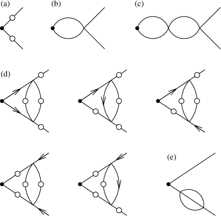
Figure 1: Diagrams appearing in the correlator $\mathbf{U}$ to second order in $u$. The heat current vertex $\mathbf{j}^{Q}$ is denoted by a black circle. A line with an arrow denotes the bare propagator $G_{0}$, and a line with an empty circle denotes the bare correlator $C_{0}$ [in (b), (c), and (e) the diagrams are shown without presenting all possible arrangements of propagator and correlator lines]. Diagram (a) is the bare (or zeroth order) contribution. Diagrams (b) and (c) are first and second order diagrams, respectively, which have a vanishing contribution. Diagrams which contribute to second order are given in (d) and (e).

At Gaussian order [see Fig. 1(a)] and to linear order in $\mathbf{q}$ and $\omega$, we have

$$\mathbf{U}_{0}=\frac{4\mathbf{q}\,\omega}{\Gamma^{2}r^{4}}.$$ (20)

To first order in $u$ we have the diagram in Fig. 1(b), but its contribution vanishes due to symmetry considerations [as does the second order diagram in Fig. 1(c)]. (Diagrams in which a closed loop appears on one of the propagators are included by the renormalization of $r$.) To second order in $u$, we have the diagrams in Fig. 1(c)–(e). Of these, we have illustrated in Fig. 1(d) the fact that each of these diagrams is in fact a set of diagrams with different placements of propagator and correlator lines. Note that the external legs in the different diagrams may be either propagator or correlator lines. For this reason, in contrast with the static case, we calculate all diagrams appearing to a given order, not only those which are irreducible with respect to the external legs.

In the calculation of the diagrams, we are interested in the infrared divergence when $r\rightarrow 0$. The diagrams are also ultraviolet divergent, which we regularize by dimensional regularization (see., e.g., Ref. Binney-etal ). The actual calculation of these diagrams is rather lengthy, and we will spare the reader the details. Very briefly, the various diagrams are evaluated using the value of $u$ at the fixed point, which to order $\epsilon$ is $u^{*}=\pi^{2}\epsilon/5$. It is convenient to express the result in terms of the exponent $\eta$ (to second order in $\epsilon$, $\eta=\epsilon^{2}/50$) and the coefficient $c=6\ln\frac{4}{3}-1$, which appears in the result for the dynamical critical exponent, $z=2+c\eta$ Halperin-Hohenberg-Ma . The result is

$$\mathbf{U}=\mathbf{U}_{0}\left(1-\frac{3}{2}(c+1)\eta\ln r\right)\propto r^{-4-3(c+1)\eta/2}.$$ (21)

A comparison of Eqs. (16) and (21) gives $d_{Q}=d+1$ to second order in $\epsilon$. We thus do not find an anomalous dimension for the heat current operator in the $\epsilon$ expansion, in agreement with the general argument given above.

IV Introducing a temperature gradient

In previous sections, the temperature $T$ was constant throughout the sample. A constant temperature may be simply absorbed by an appropriate rescaling of variables, so that it does not appear explicitly in the problem. Indeed, by rescaling the order parameter, free energy, and noise using $\psi\rightarrow\sqrt{T}\psi$, $F\rightarrow TF$, and $\zeta\rightarrow\zeta/\sqrt{T}$, Eqs. (4)–(5) may be rewritten without an explicit temperature (this also requires rescaling the coefficient of the quartic term in the free energy). This is the form traditionally used in the literature on critical dynamics Hohenberg-Halperin .

For thermal and thermoelectric transport, however, we should also consider the application of temperature gradients in the sample. For this purpose, we have retained the explicit temperature dependence of the noise correlator, Eq. (5). Other parameters of the problem may also have an implicit temperature dependence; however, at least for linear response to a temperature gradient, the dependence of parameters on temperature is not important for transport and is subsequently ignored. The reason for this is that if we ignore the temperature dependence in the noise, the system then has spatially-dependent local couplings (through their temperature dependence) but remains in isothermal equilibrium; thus it carries no transport currents.

Rescaling Eq. (3), as discussed above, leads to the following equation of motion, to linear order in the temperature gradient,

$$\frac{\partial\psi}{\partial t}=$$

$$-\,\Gamma_{0}\left[r_{0}\psi+2u_{0}|\psi|^{2}\psi-\nabla^{2}\psi-(\nabla\psi)\cdot(\nabla T)/T\right]+\zeta.$$

The dependence of the correlator (5) on temperature has been exchanged for a term proportional to $\nabla T$ in the stochastic equation. The equation may still be recast in the form (3), provided an additional term, of the form $-\mathbf{j}^{Q}\cdot\tilde{\mathbf{A}}$, is added to (the integrand of) the free energy, Eq. (4). Here, $\mathbf{j}^{Q}$ is the heat current, Eq. (1). It is coupled to a “gravitational” vector potential $\mathbf{\tilde{A}}$. The notion of a gravitational field was introduced by Luttinger Luttinger as a fictitious device for studying temperature gradients (see also Ref. Cooper-Halperin-Ruzin ). Here, we briefly discuss this point, noting the analogy between the treatment of electric and thermal currents. In particular, Einstein relations for thermal currents relate the response to $(\nabla T)/T$ with the response to a gravitational force $\tilde{\mathbf{E}}=-\nabla\tilde{\phi}$, where $\tilde{\phi}$ is Luttinger’s gravitational field. By performing a gravitational gauge transformation, the gravitational force is expressed in terms of a gravitational vector potential, $\tilde{\mathbf{E}}=-\partial\tilde{\mathbf{A}}/\partial t$. To linear order in the gravitational force, the gravitational vector potential $\tilde{\mathbf{A}}$ is then coupled to $\mathbf{j}^{Q}$ in the free energy of model A. The equation of motion (3), coupled with the Einstein relations, reproduces Eq. (IV).

This understanding of how a thermal gradient enters the free energy is useful on several fronts. First, it verifies the form of the heat current operator, Eq. (1). Second, it replaces temperature gradients with gravitational fields. Luttinger’s original motivation was to express thermal transport coefficients in terms of the corresponding correlation functions. In the next section, we follow a similar strategy for writing scaling forms for the thermal current.

V Thermal transport

In this section, we consider the critical behavior of thermal transport coefficients in model A dynamics. Using the result for the scaling dimension of the heat current from Sec. III, $d_{Q}=d+1$, we write the general scaling relations for the electric and heat currents, in presence of an electric, magnetic, and gravitational fields,

$$\mathbf{j}^{e} = \xi^{-d+1}\mathbf{f}^{e}\left[E\xi^{1+z},B\xi^{2},(\nabla\tilde{\phi})\xi^{-1+z}\right]$$ (23)

$$\mathbf{j}^{Q} = \xi^{-d-1}\mathbf{f}^{Q}\left[E\xi^{1+z},B\xi^{2},(\nabla\tilde{\phi})\xi^{-1+z}\right].$$ (24)

These equations are extensions of known results for electric transport (see, e.g., Ref. Fisher-Fisher-Huse ).

We will use these scaling relations here to deduce the critical behavior of various linear response coefficients. We note that the assumption of particle-hole symmetry implies that $\sigma_{xy}=\alpha_{xx}=\kappa_{xy}=0$ (it is necessary to break particle-hole symmetry to discuss the critical properties of these transport coefficients). For the conductivity, as well as for the magnetic susceptibility, the known results Fisher-Fisher-Huse may be confirmed,

$$\sigma_{xx}\propto\xi^{2+z-d},\qquad\chi\propto\xi^{4-d}.$$ (25)

Our result for the heat current operator now enables us to make analogous statements for transport coefficients involving the heat current operator, $\alpha_{xy}$ and $\kappa_{xx}$.

We begin with the transverse thermoelectric response $\alpha_{xy}$, which is the coefficient of interest in studying the Nernst effect. More precisely, we will consider the response to linear order in the magnetic field. This may be calculated either from the heat current response to an applied electric and magnetic field, or as the electric current response to the applied gravitational and magnetic fields. In both cases, the current which is obtained is the total current, from which magnetization contributions, which do not contribute to transport, must be subtracted Cooper-Halperin-Ruzin . For the total currents, we find

$$\frac{j_{\text{tot}}^{Q}}{EB}\propto\frac{j_{\text{tot}}^{e}}{(\nabla\tilde{\phi})B}\propto\xi^{2+z-d}.$$ (26)

The magnetization component of these total currents is given by Cooper-Halperin-Ruzin

$$j_{\text{mag}}^{Q}=\mathbf{M}\times\mathbf{E},\qquad j_{\text{mag}}^{e}=-\mathbf{M}\times\nabla\tilde{\phi}.$$ (27)

Using the result for the magnetic susceptibility above, we see that the situation is different dependent upon the value of the critical dynamical exponent.

For $d\geq 4$ mean-field exponents hold, and the dynamical critical exponent is $z=2$. In this case, the total and magnetization pieces of the current diverge with identical power laws (cf. Ref. Ussishkin-Sondhi-Huse ). The difference of two terms with identical singularities may be of the same singular behavior or a weaker one. Thus, the critical dynamics analysis presented here does not determine conclusively the power of $\alpha_{xy}$ when $z=2$. For Gaussian fluctuations, $\alpha_{xy}$ does have the same singularity as the total currents and magnetization contributions, $\alpha_{xy}/B\propto\xi^{4-d}$  Ussishkin-Sondhi-Huse . It is quite possible that the same occurs also in two dimension (where $z=2$ as well), suggesting that $\alpha_{xy}/B\propto\xi^{2}$ above the Kosterlitz-Thouless transition temperature. However, a separate analysis is required for this case which we defer to a future work.

For three dimensions, which corresponds to the actual transition in the cuprates due to interlayer coupling, the analysis of Ref. Halperin-Hohenberg-Ma gives $z=2+c\eta>2$. In this case, the magnetization currents are less singular than the total currents from which they are subtracted, and hence the result for $\alpha_{xy}$ to linear order in $B$,

$$\alpha_{xy}/B\propto\xi^{2+z-d},$$ (28)

becomes unproblematic fn-nonvanish . We note that the dimensionless ratio $T\alpha_{xy}/M$ (where $M=\chi B$ is the magnetization) diverges at the critical point as $\xi^{z-2}$.

Finally, we consider the thermal conductivity, for which we find

$$\kappa_{xx}\propto\xi^{-2+z-d}.$$ (29)

In particular, the thermal conductivity will have a singular, but non-diverging contribution in model A in three dimensions. In contrast, Vishveshwara and Fisher argued in a recent paper Vishveshwara that the thermal conductivity is analytic at the critical point using a model C formulation (which involves a conserved energy density in addition to a non-conserved order parameter). There are several things to note about this difference in the critical behavior obtained in the two works. First, the coupling of the energy variable to the order parameter is known to be irrelevant (as $\alpha<0$ with $n=2$ components of the order parameter), and we expect the critical behavior of model C to be equivalent to that of model A HHM . Second, we note that singular behavior is already obtained for the thermal conductivity for Gaussian fluctuations in model A Ussishkin-Sondhi-Huse , a result which may also be obtained from microscopics (which are energy conserving). Finally, it seems to us that in Ref. Vishveshwara , a treatment of the order parameter contribution to the heat current is absent.

VI Final comments

Our results for the critical behavior of the transverse thermoelectric response $\alpha_{xy}$ and the thermal conductivity $\kappa_{xx}$ are based on the observation that the heat current operator has no anomalous dimension. It is worth noting that both electric and heat currents share this property; in particular they are independent of the dynamical critical exponent $z$. Readers familiar with the lore of quantum critical phenomena should note that conserved currents do exhibit $z$ in their scaling dimensions at critical points; it is their corresponding densities which do not. Thus the meaning of the phrase “absence of anomalous dimension” is different in these two cases.

We briefly comment on the possibility of observing our results in experiment. In the moderately two dimensional cuprates, such as YBCO, there is evidence for a relatively large 3D-XY critical regime. In this regime our results for $\alpha_{xy}$, to linear order in the field, at temperatures approaching $T_{c}$ can be tested via measurements of the Nernst effect and the conductivity. Another possibility, instead of attempting to extract critical exponents, is to consider the dimensionless ratio $T\alpha_{xy}/M$. This ratio equals $1/2$ in the region of Gaussian fluctuations Ussishkin-Sondhi-Huse . As the temperature is decreased towards $T_{c}$, the value of this ratio increases, eventually diverging as $\xi^{z-2}$. In the highly two dimensional cuprates such as BSSCO the scaling theory is on somewhat weaker grounds due to the degeneracy between the dimensions of the total current and the magnetization. However, absent an exact cancellation, it should still correctly predict that $\alpha_{xy}$ to linear order in $B$ diverges with the same critical exponent (i.e. $\sim\xi^{2}$) as the magnetization as the Kosterlitz-Thouless transition is approached (except perhaps for a confluent logarithm at the lower critical dimension.)

In summary, we considered the critical scaling of thermal transport near the finite temperature transition to the superconducting state, within the framework of critical model A dynamics. This leads to specific predictions for the critical exponents of thermal transport coefficients, and in particular for the Nernst effect.