Ward identities for strongly coupled Eliashberg theories

Abstract

We discuss Ward identities for strongly interacting fermion systems described by Eliashberg-type theories. We show that Ward identities are not in conflict with Migdal theorem and derive diagrammatically Ward identity for a charge vertex both in a Fermi liquid, and when a Fermi liquid is destroyed at quantum criticality. We argue that Ward identity for the spin vertex cannot be obtained within Eliashberg theory.

I introduction

Conservation laws set powerful constraints on the forms of spin and charge response functions of interacting electron systems. The most useful constraints are associated with the conservation of the the total charge and the total spin of fermions, $e_{tot}$ and $S^{z}_{tot}$. The time independence of the total charge and spin implies that the charge and spin susceptibilities, $\chi_{c}(q,\omega)$ and $\chi_{s}(q,\Omega)$, respectively, should vanish at $q=0$ and any finite $\Omega$. This requirement imposes specific relations between self-energy and vertex corrections, known as Ward identities  ward ; ll ; mahan .

The subject of this paper are Ward identities for strongly interacting fermionic systems in which the self-energy is large, but is local – it depends on frequency, but not on momentum, i.e. $\Sigma(k,\omega)\approx\Sigma(\omega)$. These theories have recently been introduced, both phenomenologically and microscopically, in context of quantum criticality in high $T_{c}$ and heavy fermion materials NFL_at_QCP . Examples include marginal Fermi liquid theory mfl , gauge theories ioffe , and critical theories of CDW grilli and SDW  acs transitions with the dynamical exponent $z>1$  hertz . In the last two cases, the locality of the problem is not imposed by the original Hamiltonian, but emerges at criticality due to the fact that for $z>1$, collective spin or charge bosonic excitations are slow modes compared to electrons. The locality of the self-energy was first discovered by Eliashberg in the analysis of electron-phonon problem eliash , and low-energy electron-boson theories with $\Sigma(k,\omega)\approx\Sigma(\omega)$ bear his name. The frequency-only dependent self-energy also emerges in infinite $D$ theories of metal-insulator transition kotliar and in local theories of heavy-fermion quantum criticality piers . However in these cases, the interaction is not small compared to a fermionic bandwidth, and our analysis will not be applicable.

The issue of Ward identities for Eliashberg theories is somewhat non-trivial as these theories are justified by Migdal theorem that states that vertex corrections $\delta\Gamma/\Gamma$ should generally be small compared to $\Sigma(\omega)/\omega$. Meanwhile, Ward identities imply that $\Delta\Gamma$ and $\Sigma(\omega)$ scale with each other. We show, however, that Migdal theorem and Ward identities just probe different limiting forms of the full, momentum and frequency dependent vertex $\Gamma(q,\Omega)$. Migdal theorem states that for $v_{F}q>>\Omega$, $\delta\Gamma/\Gamma\ll\Sigma(\omega)/\omega$. Ward identity is applicable in the opposite limit of $v_{F}q\ll\Omega$, and implies that in this limit, $\delta\Gamma/\Gamma\sim\Sigma(\omega)/\omega$.

We derive in this paper the Ward identity for the charge vertex near QCP. We show that Ward identity holds both away from QCP, when the system is in the Fermi-liquid regime, and right at QCP, where the Fermi-liquid behavior may be destroyed by quantum fluctuations. We demonstrate that in the latter case, a derivation of Ward identity by explicit summation of diagrams is not straightforward and requires some care.

We also consider the $SU(2)$ Ward identity for the spin vertex. We argue that it holds near a CDW instability, but cannot be obtained within Eliashberg theory near a magnetic QCP. The argument is that the $SU(2)$ Ward identity is related to the conservation of the total electron spin. Meanwhile, Eliashberg theory near a SDW transition is based on the spin-fermion model in which a soft collective bosonic mode in the spin channel is treated as a separate spin degree of freedom which can flip an electron spin. We argue that this effective two-fluid model is justified only when the momenta of the collective bosonic mode is much larger than its frequency: $v_{F}q>>\Omega$. In this limit, Migdal theorem is valid. However, in the opposite limit $v_{F}q<<\Omega$, relevant to the $SU(2)$ Ward identity, the derivation of the two-fluid model near a magnetic QCP breaks down, i.e., spin-fermion model is just inapplicable.

The structure of the paper is the following. We first discuss in the Sec.II how Ward identities are related to the conservation laws. In Sec III we demonstrate that Ward identities are not in conflict with Migdal theorem. In Sec. IV we derive Ward identity for the charge vertex and discuss the difference between a Fermi liquid and a non-Fermi liquid. In Sec. V we discuss in some detail Ward identity for the spin vertex.

II Ward identities and the conservation laws

For $\Sigma(k,\omega)=\Sigma(\omega)$, the full fermion-boson vertex $\Gamma$ depends on incoming and outgoing fermionic frequencies $\omega$ and $\Omega+\omega$ ($\Omega$ is a bosonic frequency), and on a bosonic momentum $q$. Its dependence on fermionic momenta is small by Migdal condition and can be neglected. The relevant Ward identity relates the self-energy with $\Gamma(q,\omega,\Omega)$ at zero bosonic momentum $q$: $\Gamma(q=0,\omega,\Omega)=\Gamma(\omega,\Omega)$. The identity implies that ll ; mahan

$$\Gamma(\omega,\Omega)=\frac{{\tilde{\Sigma}}(\omega+\Omega)-{\tilde{\Sigma}}(\omega)}{\Omega}$$ (1)

where ${\tilde{\Sigma}}(\omega)=\omega+\Sigma(\omega)$ We use the normalization in which $\Gamma=1$ for non-interacting fermions. The role of (1) in enforcing the conservation laws becomes clear when one considers a fully renormalized particle-hole polarization bubble $\Pi(q,\Omega)$ at $q=0$. Both spin and charge susceptibilities scale with $\Pi(q,\Omega)$. In the RPA approximation, $\chi_{s}(q,\Omega)=2\Pi(q,\Omega)/(1-U\Pi(q,\Omega))$, while $\chi_{c}(q,\Omega)=2\Pi(q,\Omega)/(1+U\Pi(q,\Omega))$. Hence, if $\Pi(0,\Omega)$ vanishes, $\chi_{s}(0,\Omega)$ and $\chi_{c}(0,\Omega)$ also vanish.

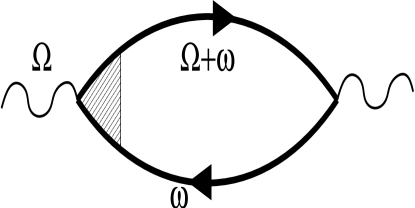
Figure 1: The full particle-hole polarization bubble. Solid lines – full Green’s functions, black triangle - the full vertex $\Gamma(\omega,\Omega)$.

The proof that $\Pi(0,\Omega_{m})$ vanishes for Eliashberg-type theories has not been presented in the literature, so we discuss the computation in some detail. The full polarization bubble in Matsubara frequencies is given by the diagram in Fig.1

$$\Pi(0,\Omega_{m}) = -\int\int\frac{d^{D}pd\omega_{m}}{(2\pi)^{D+1}}\times$$ (2)

$$\Gamma(\omega_{m},\Omega_{m})G(p,\omega_{m})G(p,\omega_{m}+\Omega_{m})$$

where the fermionic Green’s function $G(p,\omega_{m})$ is given by

$$G(p,\omega_{m})=\left(i{\tilde{\Sigma}}(\omega_{m})-\epsilon_{p}\right)^{-1}.$$ (3)

Linearizing, as usual, the dispersion near the Fermi surface as $\epsilon_{p}=v_{F}(p-p_{F})$, and replacing the momentum integral $\int d^{D}p/(2\pi)^{D}$ by $N_{0}\int d\epsilon_{p}$, we obtain from (2):

$$\Pi(0,\Omega_{m})=-N_{0}\int\frac{d\omega_{m}}{2\pi}\Gamma(\omega_{m},\Omega_{m})\times$$

$$\int_{-W}^{W}d\epsilon_{p}\frac{1}{(\epsilon_{p}-i{\tilde{\Sigma}}(\omega_{m}))(\epsilon_{p}-i{\tilde{\Sigma}}(\omega_{m}+\Omega_{m}))}$$ (4)

where $W$ is of order of fermionic bandwidth. It is common to set $W$ infinite in continuous theories. We will see, however, that it is important to keep $W$ finite at intermediate stages of calculations, and set $W=\infty$ only at the very end. The need for this procedure follows from the fact that at large frequencies ${\tilde{\Sigma}}(\omega_{m})\approx\omega_{m}$, $\Gamma\approx 1$, and the 2D integral over $d\epsilon_{p}d\omega_{m}$ formally diverges. A finite $W$ provides the physical regularization of the divergence as the linearization of the dispersion is only valid at $v_{F}(p-p_{F})\leq E_{F}$. The frequency integral, on the other hand, has to be evaluated in infinite limits.

Integrating explicitly over $\epsilon_{p}$ in (4) we obtain

$$\Pi(0,\Omega_{m})=iN_{0}\int^{\infty}_{-\infty}\frac{d\omega_{m}}{2\pi}\frac{\Gamma(\omega_{m},\Omega_{m})}{{\tilde{\Sigma}}(\omega_{m}+\Omega_{m})-{\tilde{\Sigma}}(\omega_{m})}~{}\log{\frac{(W-i{\tilde{\Sigma}}(\omega_{m}+\Omega_{m}))(-W-i{\tilde{\Sigma}}(\omega_{m}))}{(-W-i{\tilde{\Sigma}}(\omega_{m}+\Omega_{m}))(W-i{\tilde{\Sigma}}(\omega_{m}))}}$$ (5)

One can easily make sure that at $W\rightarrow\infty$, the frequency integral in (5) is the sum of two terms: $\Pi(0,\Omega_{m})=\Pi_{1}(0,\Omega_{m})+\Pi_{2}(0,\Omega_{m})$. The first contribution comes from large $\omega_{m}\gg\Omega_{m}$ for which ${\tilde{\Sigma}}(\omega)\sim W$. Expanding in ${\tilde{\Sigma}}(\omega+\Omega)-{\tilde{\Sigma}}(\omega)$ in the logarithm, we obtain

$$\Pi_{1}(0,\Omega_{m})=4N_{0}\int_{0}^{\infty}\Gamma(\omega_{m},\Omega_{m})\frac{W}{W^{2}+{\tilde{\Sigma}}^{2}(\omega_{m})}\frac{d\omega}{2\pi}$$ (6)

The integrand is $O(1/W)$ up to ${\tilde{\Sigma}}(\omega)\sim W$, and $O(W/{\tilde{\Sigma}}^{2}(\omega))$ at larger frequencies. This implies that the integral is confined to $\omega$, for which ${\tilde{\Sigma}}(\omega)\sim W$. At these frequencies both the self-energy and the vertex renormalization are irrelevant, i.e., $\Gamma(\omega_{m},\Omega_{m})=1$, and ${\tilde{\Sigma}}(\omega_{m})=\omega_{m}$. Performing the frequency integration in (6) we then obtain

$$\Pi_{1}(0,\Omega_{m})=4N_{0}\int_{0}^{\infty}\frac{W}{W^{2}+\omega^{2}_{m}}\frac{d\omega}{2\pi}=N_{0}$$ (7)

Another contribution comes from small frequencies $\omega_{m}\sim\Omega_{m}$, when $\omega_{m}$ and $\omega_{m}+\Omega_{m}$ have different signs, and the argument of the logarithm is $i\pi~{}(sgn(\omega+\Omega)-sgn\omega)$. The real part of the logarithm is $O(1/W)$ at small frequencies and can be neglected. Replacing the logarithm in (5) by its argument, we obtain

$$\Pi_{2}(0,\Omega_{m})=-N_{0}\int_{-\Omega_{m}}^{0}d\omega~{}\frac{\Gamma(\omega_{m},\Omega_{m})}{{\tilde{\Sigma}}(\omega_{m}+\Omega_{m})-{\tilde{\Sigma}}(\omega_{m})}~{}$$ (8)

For definiteness, we set $\Omega_{m}>0$. Using Ward identity, Eq. (1), we immediately obtain

$$\Pi_{2}(0,\Omega_{m})=-N_{0}\int_{0}^{\Omega_{m}}\frac{d\omega_{m}}{\Omega_{m}}=-N_{0}$$ (9)

Comparing (7) and (9), we see that the low frequency contribution, for which Ward identity is crucial, cancels the one from high frequencies, and, as a result, $\Pi(0,\Omega_{m})$ vanishes, as it indeed should.

Figure 2: The lowest-order diagrams for the fermionic self-energy and fermion-boson vertex. Wavy line is the bosonic propagator $\chi_{l}(\omega)$.

III Diagrammatic derivation of Ward identity

III.1 the relation to Migdal theorem

A more subtle issue is how to prove Eq. (1) diagrammatically. A conventional recipe is to relate the equations for the full vertex and the fermionic self-energy ll ; mahan . At a first glance, this would contradict Migdal theorem that states that in Eliashberg-type theories, vertex corrections are much smaller than the self-energy. migdal . We will demonstrate, however, that Migdal theorem is only valid for $v_{F}q\gg\Omega$, while Eq. (1) is valid for $v_{F}q\ll\Omega$. To understand the importance of the $v_{F}q/\Omega$ ratio, note that every Eliashberg-type theory can be viewed as the interaction between fermions and the “local” spin or charge bosonic propagator $\chi_{l}(\Omega)=\int dq^{d-1}\chi(q,\Omega)$ ioffe ; acs ; cmhf ; catherine ; finn . The lowest order self-energy and vertex corrections due to electron-boson interaction are shown in Fig. 2. For the self-energy, we have acs

$$\Sigma(\omega_{m})\propto g^{2}N_{0}\int d\epsilon_{k}\int d\Omega_{m}G_{0}(k,\omega^{\prime}_{m}+\Omega_{m})\chi_{l}(\Omega_{m})$$ (10)

Evaluating the momentum integral using

$$\int d\epsilon_{k}G_{0}(k,\omega_{m})=\int\frac{d\epsilon_{k}}{i\omega_{m}-\epsilon_{k}}=-i\pi N_{0}sgn\omega_{m}$$ (11)

we obtain

$$\Sigma(\omega_{m})\propto g^{2}\int_{-\omega_{m}}^{0}d\Omega_{m}\chi_{l}(\Omega_{m})$$ (12)

We see that the frequency integral is confined to internal frequencies which are smaller than the external one. When $\omega_{m}$ is small, relevant $\Omega_{m}$ are also small, and away from the critical point $\chi_{l}(\Omega_{m})$ can be approximated by $\chi_{l}(0)$. Then

$$\Sigma(\omega_{m})=\lambda\omega_{m},$$ (13)

where $\lambda\propto g^{2}N_{0}\chi_{l}(0)$. When $\lambda\geq 1$, $\partial\Sigma(\omega)/\partial\omega=\lambda$ is not small. Note that Eq. (12) does not change if we re-evaluate the self-energy using the full Green’s function $G(k,\omega)=(i{\tilde{\Sigma}}(\omega)-\epsilon_{k})^{-1}$ for intermediate fermion. This follows from the observation that the relation (11) remains valid for full $G$.

For vertex correction, when both $q$ and $\Omega$ are nonzero, we have

$$\delta\Gamma(q,\omega_{m},\Omega_{m})\propto ig^{2}\int\int d^{D}kd\omega^{\prime}_{m}\times$$

$$~{}G_{0}(k,\omega^{\prime}_{m})G_{0}(k+q,\omega^{\prime}_{m}+\Omega_{m})\chi_{l}(\omega_{m}-\omega^{\prime}_{m})$$ (14)

This integral is ultraviolet convergent, and hence momentum integral can be extended to infinity. Integrating over momentum first, we obtain

$$\delta\Gamma(q,\omega_{m},\Omega_{m})\propto\frac{g^{2}N_{0}}{{\sqrt{\Omega^{2}_{m}+(v_{F}q)^{2}}}}~{}\int_{-\Omega_{m}}^{0}d\omega_{m}^{\prime}\chi_{l}(\omega_{m}-\omega^{\prime}_{m})$$ (15)

We see that the integral over internal frequency $\omega^{\prime}_{m}$ is again confined to $|\omega^{\prime}_{m}|<\Omega_{m}$. Assuming that both $\Omega_{m}$ and $\omega_{m}$ are small, we again can approximate $\chi_{l}(\omega_{m}-\omega^{\prime})$ by $\chi_{l}(0)$ and obtain

$$\delta\Gamma(q,\omega_{m},\Omega_{m})\propto\lambda\frac{\Omega_{m}}{\sqrt{\Omega^{2}_{m}+(v_{F}q)^{2}}}$$ (16)

We see that in the limit of vanishing $q$, $\Delta\Gamma\sim\lambda$ i.e., $\delta\Gamma\sim\partial\Sigma(\omega)/\partial\omega$. This is consistent with Ward identity, Eq. (1). However, in the opposite limit $v_{F}q\gg\Omega$, $\delta\Gamma$ is reduced by $\Omega/v_{F}q$. For on-shell bosons, $\Omega=uq$, where $u$ is the effective “sound” velocity comm Hence, $\Delta\Gamma\sim\lambda u/v_{F}$. The ratio $u/v_{F}$ is a small parameter in Eliashberg-type theories mahan ; migdal , and the strong coupling limit of these theories implies that $\lambda>1$, while $\lambda u/v_{F}\ll 1$. In this limit, the vertex for the scattering of fermions by on-shell bosons is small, in agreement with Migdal theorem.

Figure 3: The second-order diagrams for the boson-fermion vertex $\Gamma(\omega,\Omega)$: (a) ladder diagram, (b) crossed diagram, (b) the diagram with the renormalization of the side vertex. For Eliashberg theories, the ladder diagram is much larger than the other two.

III.2 the selection of the diagrams

The next issue is how to select series of diagrams for $\delta\Gamma(q,\omega_{m},\Omega_{m})$. A simple experimentation shows that for $\lambda u/v_{F}\ll 1$, relevant diagrams for vertex renormalization form ladder series in which each fermionic propagator is the full one. All non-ladder diagrams are small in $\lambda u/v_{F}$. To demonstrate this, compare the two second-order diagrams for $\delta\Gamma(q,\omega_{m},\Omega_{m})$ - the ladder diagram and the crossed diagram (see Fig.3 a, b). For both diagrams, we consider the limit when both $q$ and $\Omega_{m}$ are small, but $v_{F}q\ll\Omega_{m}$. The ladder diagram $\delta\Gamma^{(2)}_{L}$ can be straightforwardly calculated in the same way as above and yields $\delta\Gamma^{(2)}_{L}\sim\lambda^{2}$. For the crossed diagram $\delta\Gamma^{(2)}_{C}$, we have, setting external $\omega_{m}=0$ and $|{\bf k}_{ext}|=k_{F}$,

$$\delta\Gamma^{{(2)}}_{C}\propto g^{4}\int d^{D}kd^{D}pd\omega^{\prime}_{m}d\omega^{\prime\prime}_{m}G_{0}({\bf k},\omega^{\prime}_{m})G_{0}({\bf k}+{\bf q},\omega^{\prime}_{m}+\Omega_{m})~{}G_{0}({\bf p},\omega^{\prime\prime}_{m})G_{0}({\bf k}_{ext}+{\bf k}-{\bf p},\omega^{\prime}_{m}-\omega^{\prime\prime}_{m})~{}\chi_{l}(\omega^{\prime}_{m}+\Omega-\omega^{\prime\prime}_{m})~{}\chi_{l}(\omega^{\prime\prime}_{m})$$ (17)

The integration over ${\bf k}$ and $\omega^{\prime}_{m}$ proceeds in the same way as before and yields a factor of $\lambda$. The integral comes from vanishingly small $\omega^{\prime}\leq\Omega_{m}$, hence $\omega^{\prime}$ can be neglected in the rest of the diagram. The remaining integral then reduces to

$$\delta\Gamma^{{(2)}}_{C} \propto \lambda\frac{g^{2}}{\chi_{l}(0)}\int d^{D}pd\theta d\omega^{\prime\prime}_{m}$$ (18)

$$\times G_{0}({\bf p},\omega^{\prime\prime}_{m})G_{0}({\bf l}-{\bf p},-\omega^{\prime\prime}_{m})~{}\chi^{2}_{l}(\omega^{\prime\prime}_{m})$$

where ${\bf l}={\bf k}_{ext}+{\bf k}$ is a vector whose length is $2k_{F}\cos\theta$. To avoid large denominators in the integrand in (18), both ${\bf p}$ and ${\bf l}-{\bf p}$ must be near the Fermi surface. For each given ${\bf l}$, this selects special hot regions on the Fermi surface. The Fermi velocities at ${\bf p}$ and ${\bf l}-{\bf p}$ in these two regions are generically not aligned, hence, in evaluating the momentum integral in (18), one has to integrate independently over $\epsilon_{\bf p}$ and $\epsilon_{{\bf l}-{\bf p}}$. Using $\int d^{D}p\propto(N_{0}/W)\int\int d\epsilon_{\bf p}d\epsilon_{{\bf l}-{\bf p}}$ and integrating each of the two Green’s functions in (18) over its $\epsilon$ we obtain

$$\delta\Gamma^{{(2)}}_{cr}\propto\lambda^{2}~{}\chi^{2}_{l}(0)\int\frac{d\omega^{\prime\prime}_{m}}{W}~{}\left(f(\omega^{\prime\prime}_{m})\right)^{2}$$ (19)

where we introduced $f(\omega)=\chi_{l}(\omega)/\chi_{l}(0)$, $f(0)=1$.

The frequency integral converges at $\omega^{\prime\prime}\sim up_{F}$ such that the frequency integral gives $up_{F}/W\sim u/v_{F}$. Substituting this into (19), we find that $\delta\Gamma^{{(2)}}_{cr}\sim\lambda[\lambda(u/v_{F})]$, i.e., it is small compared to ladder diagrams. One can verify that the same smallness in $\lambda u/v_{F}$ emerges when one includes the renormalization of the side vertices in the ladder series (see Fig.3 c).

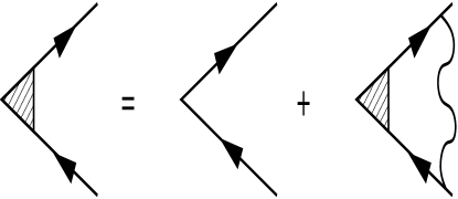
Figure 4: The series of ladder diagrams for the full fermion-boson vertex. The diagrammatic series reduce to the integral equation for $\Gamma$.

To prove Eq. (1) we now need to go beyond estimates and explicitly sum up ladder series of diagrams. At this stage, we consider charge and spin vertices separately.

IV The charge vertex

IV.1 general proof

We begin with the charge vertex $\Gamma_{c}(q=0)$. The bosonic $\chi_{l}(\omega)$ may originate either in the charge or in the spin channel. In both cases, we define $\lambda$ via $\Sigma(\omega_{m})=\lambda\omega$ at small $\omega$. For charge fluctuations, $\lambda=g^{2}N_{0}\chi_{l}(0)$, for spin fluctuations, $\lambda=3g^{2}N_{0}\chi_{l}(0)$. Evaluating the lowest order perturbative correction to the charge vertex, we find that at small $\Omega_{m}$ and $\omega_{m}$, $\Gamma_{c}(\omega_{m},\Omega_{m})=1+\lambda$, i.e., vertex renormalization contains exactly the same $\lambda$ independently on whether $\chi_{l}(\omega)$ is of spin or charge origin.

Further, the ladder series of of vertex correction diagrams reduce to the integral equation for $\Gamma_{c}(\omega_{m},\Omega_{m})$ in the form

$$\Gamma_{c}(\omega_{m},\Omega_{m})=1+i\lambda\int\int\frac{d\epsilon_{k}d\omega^{\prime}_{m}}{2\pi}~{}f(\omega_{m}-\omega^{\prime}_{m})\times$$

$$\frac{\Gamma_{c}(\omega^{\prime}_{m},\Omega_{m})}{(i{\tilde{\Sigma}}(\omega^{\prime}_{m})-\epsilon_{k})(i{\tilde{\Sigma}}(\Omega_{m}+\omega^{\prime}_{m})-\epsilon_{k})}$$ (20)

We show this graphically in Fig. 4.

A similar equation can be obtained for the self-energy. Explicitly computing the prefactor in (15) and using the fact that the self-energy given by (15) does not change if we replace $G_{0}$ by full $G$, as long as $\Sigma$ depends only on frequency, we obtain

$${\tilde{\Sigma}}(\omega_{m}+\Omega_{m})-{\tilde{\Sigma}}(\omega_{m})=\Omega_{m}+i\lambda\int\int\frac{d\epsilon_{k}d\omega^{\prime}_{m}}{2\pi}~{}\times$$

$$\frac{{\tilde{\Sigma}}(\Omega_{m}+\omega^{\prime}_{m})-{\tilde{\Sigma}}(\omega^{\prime}_{m})}{(i{\tilde{\Sigma}}(\omega^{\prime}_{m})-\epsilon_{k})(i{\tilde{\Sigma}}(\Omega_{m}+\omega^{\prime}_{m})-\epsilon_{k})}~{}f(\omega_{m}-\omega^{\prime}_{m})$$ (21)

Comparing Eqs. (21) and (20), we see that they are equivalent if $\Gamma_{c}(\omega_{m},\Omega_{m})=({\tilde{\Sigma}}(\omega_{m}+\Omega_{m})-{\tilde{\Sigma}}(\omega_{m}))/\Omega_{m}$, i.e., when $\Sigma(\omega_{m})$ and $\Gamma_{c}(\omega_{m},\Omega_{m})$ are related by Ward identity – Eq. (1).

IV.2 perturbation theory order by order

It is also instructive to analyze how Eq. (1) is recovered by summing up vertex correction diagrams explicitly, order by order, and comparing the result with the self-energy. Order by order consideration was used to prove Ward identity for electron-phonon systems mahan . There, series of vertex corrections are geometrical and one can straightforwardly sum them up. We will see that in our case, the series of vertex corrections are geometrical in the Fermi liquid regime, but become non-geometrical at the QCP, where $\lambda=\infty$. In the last case, explicit order by order summation of perturbation series is not straightforward and requires some efforts.

IV.2.1 Fermi liquid

In a Fermi liquid, $f(\omega)\approx 1$, and ${\tilde{\Sigma}}(\omega)=\omega_{m}(1+\lambda)$. Then the leading vertex correction calculated with the full fermionic propagators is $\lambda/(1+\lambda)$. One can easily make sure that higher-order vertex corrections form simple geometrical series in $\lambda/(1+\lambda)$. Adding them up, we immediately obtain

$$\Gamma_{c}(q=0)=\frac{\lambda}{1+\lambda}+\left(\frac{\lambda}{1+\lambda}\right)^{2}+...=\frac{1}{1-\frac{\lambda}{1+\lambda}}$$

$$=1+\lambda=\frac{{\tilde{\Sigma}}(\omega+\Omega)-{\tilde{\Sigma}}(\omega)}{\Omega}$$ (22)

IV.2.2 quantum-critical point

Suppose now that the system approaches a QCP at which the bosonic mode becomes massless. If the spatial dimension is below the critical one $d_{cr}$, the local susceptibility $\chi_{l}(0)$ diverges at QCP what implies that $\lambda->\infty$ ($d_{cr}=3$ for Ornstein-Zernike form of $\chi(q,0)$ acs ; finn ). Suppose further that at QCP, the local susceptibility behaves as $\chi_{l}(\omega_{m})\propto\omega_{m}^{-\gamma}$, and $\gamma>0$. Examples include 3D antiferromagnetic and ferromagnetic QCP millis_roussev ; bedell and marginal Fermi liquid theory mfl , where $\gamma=0+$ (i.e., $\chi_{l}(\omega_{m})\propto\log\omega$), 2D antiferromagnetic QCP where $\gamma=1/2$ acs ; finn , ferromagnetic QCP cmhf ; catherine ; lonz ; gorkov and gauge theory ioffe , where $\gamma=1/3$, and corresponding CDW instabilities with the same $\gamma$ grilli ; lonz . In all density-wave cases, upper critical dimension is $D_{cr}=3$.

For $\chi_{l}(\omega_{m})\propto\omega_{m}^{-\gamma}$, self-energy acquires a non-Fermi liquid form

$$\Sigma(\omega_{m})=\omega^{1-\gamma}_{m}\omega^{\gamma}_{0},$$ (23)

where $\omega_{0}$ is the normalization factor. Ward identity implies that the fully renormalized vertex should behave as $\Gamma\propto\omega^{-\gamma}$, i.e., it should diverge at $\omega=0$.

Substituting this self-energy into (20) and evaluating vertex corrections iteratively, order by order, we obtain for $\Omega_{m},\omega_{m}>0$,

$$\Gamma_{c}(\omega_{m},\Omega_{m})=1+(1-\gamma)\int_{0}^{1}\frac{dx}{(x+\frac{\omega_{m}}{\Omega_{m}})^{\gamma}}~{}\frac{1}{S(x)}\left[1+(1-\gamma)\int_{0}^{1}\frac{dy}{|x-y|^{\gamma}}~{}\frac{1}{S(y)}\left[1+(1-\gamma)\int_{0}^{1}\frac{dz}{|y-z|^{\gamma}}~{}\frac{1}{S(z)}+....\right]\right]$$ (24)

where $S(x)=(\Omega_{m}/\omega_{0})^{\gamma}+x^{1-\gamma}+(1-x)^{1-\gamma}$. Evaluating the first few terms, we obtain for, e.g., $\gamma=1/2$ and $\omega_{m}=\Omega_{m}=0$:

$$\Gamma_{c}(0,0)=1+0.7854+0.7578+...$$ (25)

Clearly, the series are not geometrical, and first few terms do not give a hint what the full $\Gamma_{c}(0,0)$ actually diverges. This implies that the direct, order by order summation of vertex correction diagrams is useless at the QCP.

Despite that order by order summation fails, infinite series in (24) can indeed be evaluated explicitly. For this we introduce $\phi(x)$ via

$$\Gamma_{c}(\omega_{m},\Omega_{m})=1+(1-\gamma)\int_{0}^{1}\frac{dx}{(x+\frac{\omega_{m}}{\Omega_{m}})^{\gamma}}\frac{\phi(x)}{S(x)}$$ (26)

and observe that $\phi(x)$ obeys the integral equation

$$\phi(x)=1+(1-\gamma)\int_{0}^{1}\frac{dy}{|x-y|^{\gamma}}~{}\frac{\phi(y)}{S(y)}$$ (27)

One can verify that the solution of (27) is $\phi(x)=S(x)(\omega_{0}/\Omega_{m})^{\gamma}$. Substituting this $\phi(x)$ into (26) and performing the integration, we obtain

$$\Gamma_{c}(\omega_{m},\Omega_{m})=1+\left(\frac{\omega_{0}}{\Omega_{m}}\right)^{\gamma}\left[\left(1+\frac{\omega_{m}}{\Omega_{m}}\right)^{1-\gamma}-\left(\frac{\omega_{m}}{\Omega_{m}}\right)^{1-\gamma}\right]$$ (28)

This is precisely the same result as one would obtain by substituting the self-energy, Eq. (23), into Eq. (1). In particular, when $\Omega_{m}$ tends to zero, and $\omega_{m}\sim\Omega_{m}$, the full charge vertex diverges as $\Omega_{m}^{-\gamma}$.

V The spin vertex

Finally, we discuss the spin vertex $\Gamma_{s}$. Here the situation is more involved. When $\chi_{l}$ originates in the charge channel, as e.g., near CDW instability grilli , the spin factors in the self-energy and the vertex correction diagrams are the same (both equal to one), and Ward identity for $\Gamma_{s}$ readily follows from the summation of the ladder series of diagrams. However, if $\chi_{l}$ originates in the spin channel, as near a SDW instability acs , the interplay between the self-energy and the vertex corrections depends on the spatial anisotropy of $\chi_{l}$. If the SDW transition is of Ising type, i.e., only the $z-$ component of $\chi_{l}$ is relevant, the spin summation yields the same factor $1$ both for the self-energy and the vertex millis_roussev ; bedell ; cmhf , and the ladder summation recovers Eq. 1. However, if the transition falls into Heisenberg universality class, the summation over spin components in the first self-energy diagram yields a factor $\sum_{\beta}{\vec{\sigma}}_{\alpha,\beta}{\vec{\sigma}}_{\beta,\alpha}=3$, while the summation over spin components in the first vertex correction diagram yields a factor $(-1)$ as $\sum_{\alpha,\beta}\sigma^{i}_{\alpha,\beta}{\vec{\sigma}}_{\beta,\gamma}{\vec{\sigma}}_{\delta,\alpha}=-\sigma^{i}_{\delta,\gamma}$ cmhf . As a result, the analogy between self-energy and vertex correction diagrams is lost for $\Gamma_{s}$. In a Fermi liquid, ladder diagrams for $\Gamma_{s}$ now form series in $-(1/3)\lambda/(1+\lambda)$, and the summation of the ladder series yields $\Gamma_{s}=3(1+\lambda)/(3+4\lambda)$ what is different from $1+\lambda$ expected from Eq. 1.

The fact that Eq. (1) for $\Gamma_{s}$ is not recovered in the summation of the ladder diagrams does not imply that the Ward identity based on the conservation of the total $S^{z}$ is invalid. Rather, the non-equivalence between self-energy and vertex corrections is the consequence of the fact that for spin vertex, Eliashberg theory near the SDW instability is only applicable for $v_{F}q\gg\Omega$, but not at $\Omega\gg v_{F}q$ where Ward identity must be valid. Indeed, the point of departure for the SDW Eliashberg theory is the spin-fermion model hertz ; acs . This model assumes that the low-energy physics is governed by the vector spin-spin interaction

$${\cal H}_{int}=g\sum_{q}{\bf s}(q){\bf S}(q)$$ (29)

between a fermion with a spin ${\bf s}(q)=\sum_{k}c^{\dagger}_{k,\alpha}{\bf\sigma}_{\alpha,\beta}c_{k+q,\beta}$ and a spin collective mode described by a bosonic field ${\bf S}(q)$. In other words, a static collective mode is formally treated as a separate spin degree of freedom. Within this description, the total spin of the system is ${\bf S}_{tot}(q)={\bf s}(q)+{\bf S}(q)$. This total spin is indeed a conserved quantity. However, the Ward identity, Eq. (1), involves only the electron spin as is evident from its relation to the electron particle-hole polarization bubble $\Pi(q,\Omega)$. If the interaction with the collective mode is of Ising type, there are no spin-flip processes between $s^{z}(q)$ and $S^{z}(q)$, and $s^{z}(q=0)$ and $S^{z}(q=0)$ are two independent conserved quantities. In this situation, Eq. (1) is satisfied, as we have demonstrated above. However, for Heisenberg-type exchange with the collective mode, only ${\bf S}^{z}_{tot}(0)$ is conserved, but not $s^{z}(0)$ as the electron spin can flip under the action of $S^{+}(q)s^{-}(q)$ and transfer its $z$ component to ${\bf S}(q)$. As a result, within the spin-fermion model, there is no conservation of the electron spin.

In reality, ${\bf S}$ is indeed an auxiliary field. Collective modes are made out of electrons, so there is no independent spin degrees of freedom other than electron spins. The physics behind the effective spin-fermion model with two spin degrees of freedom is the separation of scales. In perturbation series, the static part of the spin susceptibility comes predominantly from electrons with energies comparable to the fermionic bandwidth $W\sim v_{F}p_{F}$, while the dynamics of the spin response function is dominated by the Landau damping and comes from fermions, with energies comparable to the frequency of the collective mode $\Omega$. Eq. (29) is valid if relevant $\Omega$ are much smaller than $W$. The largest bosonic momenta are of order $p_{F}$, hence the largest $\Omega$ for typical, mass shell bosons is of order $up_{F}$. The condition $\Omega<<W$ then implies $u<<v_{F}$, which is precisely the applicability condition for Eliashberg theory. This condition, however, also implies that at small $q$, typical $\Omega\sim uq\ll v_{F}q$, i.e., the limit of $q=0$ and finite $\Omega$, relevant for the conservation laws, cannot be reached.

VI conclusions

To summarize, in this paper we considered Ward identities for charge and spin vertices in strongly coupled Eliashberg-type theories in which $\Sigma(k,\omega)\approx\Sigma(\omega)$. We explicitly demonstrated how Ward identities impose conservation laws and argued that Ward identities are not in conflict with Migdal theorem. For the charge vertex, we demonstrated that Ward identity is reproduced by summing up ladder series of diagrams, both in the Fermi liquid regime, and when the Fermi liquid is destroyed at either CDW or SDW QCP. We found, however, that order-by-order summation is only useful in the Fermi liquid regime, but becomes meaningless at the QCP. For the spin vertex, we found that Ward identity is reproduced near a CDW transition and near an Ising-type SDW transition, but cannot be reproduced near a Heisenberg-type SDW transition. We argued that this is the consequence of the fact that Eliashberg theory near a Heisenberg SDW transition is only valid when the bosonic momentum is much larger than the bosonic frequency, $v_{F}q>\Omega$. Ward identity, on the contrary, is valid in the the opposite limit $v_{F}q<\Omega$, where Eliashberg theory is inapplicable.

This work was supported by NSF DMR 0240238. I thank Ar. Abanov, C. Castellani, C. DiCastro, M. Grilli, D. Maslov, C. Pepin, J. Rech and R. Ramazashvili for useful conversations.

References

- (1) J.C. Ward, Phys. Rev. 78, 182 (1950).
- (2) E.M. Lifshitz and L.P. Pitaevskii, Statistical physics, Pergamon Press, Oxford, 1980.
- (3) G.D. Mahan, Many-Particle Physics, Plenum Press, 1990.
- (4) S. Sachdev, Quantum Phase Transitions, Cambridge University Press (Cambridge, 1999).
- (5) J.A. Hertz, Phys. Rev. B 14, 1165 (1976); A. Millis, Phys. Rev. B 48, 7183 (1993); T. Moriya, “Spin fluctuations in itinerant electron magnetism”, Springer-Verlag, 1985.
- (6) C. M. Varma, P.B. Littlewood, S. Schmitt-Rink, E. Abrahams, A. E. Ruckenstein, Phys. Rev. B 63, 1996 (1989); Phys. Rev. Lett. 64, 497 (1990).
- (7) see e.g., A. Georges et al, Rev. Mod. Phys. , 68, 13 (1996).
- (8) P. Coleman , C. Pepin, Q. Si , R. Ramazashvili, Journal of Physics: Condensed Matter 13, 723-738, (2001).
- (9) B. Altshuler, L.B. Ioffe and A.J. Millis, Phys. Rev. B 52, 5563 (1995).
- (10) C. Castellani, C. DiCastro, and M. Grilli, Z. Phys. B 103, 137 (1997). S. Caprara, M. Sulpizi, A. Bianconi, C. Di Castro and M. Grilli, Phys. Rev. B 59, 14980 (1999); A. Perali, C. Castellani, C. Di Castro, M. Grilli, E. Piegari and A.A. Varlamov, Phys. Rev. B 62, R9295 (2000); S. Andergassen, S. Caprara, C. Di Castro and M. Grilli, Phys. Rev. Lett. 87, 056401-1 (2001).
- (11) A. Abanov, A.V. Chubukov and J. Schmalian, Adv. Phys. 52, 119 (2003); A. V. Chubukov, D. Pines and J. Schmalian, in “The physics of Superconductors”, K.H. Bennemann and J.B. Ketterson eds, Springer, 2003, vol. 1, p. 495.
- (12) G.M. Eliashberg, Sov. Phys. JETP 11, 696 (1960), Sov. Phys. JETP 16, 780 (1963); D.J. Scalapino in Superconductivity, Vol. 1, p. 449, Ed. R. D. Parks, Dekker Inc. N.Y. 1969; F. Marsiglio and J.P. Carbotte, in ‘The Physics of Conventional and Unconventional Superconductors’, Eds. K.H. Bennemann and J.B. Ketterson (Springer-Verlag).
- (13) R. Roussev and A. J. Millis, Phys. Rev. B 63, 140504 (2001).
- (14) Z. Wang, W. Mao and K. Bedell, Phys. Rev. Lett. 87, 257001 (2001).
- (15) A. Chubukov, A. Finkelstein, R. Haslinger and D. Morr, Phys. Rev. Lett. 90, 077002 (2003).
- (16) A. Migdal, Soviet Physics JETP 7, 996-1001 (1958).
- (17) A. Chubukov. C. Pepin and J. Rech, Phys. Rev. Lett. 92, 147003 (2004).
- (18) Ar. Abanov, A. V. Chubukov, and A. Finkelstein, Europhys. Lett., Phys. 54, 488 (2001).
- (19) P. Monthoux and G.G. Lonzarich, Phys. Rev. B 69, 064517 (2004).
- (20) M. Dzero and L.P. Gorkov, cond-mat/0310124.
- (21) For overdamped, diffusive bosons by itself scales as some power of (as near a critical point at a finite and as near a critical point at ). In this situation, the choice of the effective velocity depends on what kind of problem is considered. Thus, for a pairing problem near QCP, relevant frequencies are of order of fermion-boson interaction ioffe ; grilli ; acs ; cmhf ; catherine ; finn ; lonz ), hence relevant momenta are determined from . In all cases studied so far ioffe ; grilli ; acs ; cmhf ; catherine ; finn ; lonz ; gorkov ) Eliashberg condition is valid when .