Extracting the electron–boson spectral function $\alpha^{2}$F($\omega$) from infrared and photoemission data using inverse theory

Abstract

We present a new method of extracting electron-boson spectral function $\alpha^{2}$F($\omega$) from infrared and photoemission data. This procedure is based on inverse theory and will be shown to be superior to previous techniques. Numerical implementation of the algorithm is presented in detail and then used to accurately determine the doping and temperature dependence of the spectral function in several families of high-T_c superconductors. Principal limitations of extracting $\alpha^{2}$F($\omega$) from experimental data will be pointed out. We directly compare the IR and ARPES $\alpha^{2}$F($\omega$) and discuss the resonance structure in the spectra in terms of existing theoretical models.

I Introduction

The electron-boson spectral function is one of the most important properties of a BCS superconductor carbotte90 . In conventional superconductors the electron-phonon spectral function has been successfully obtained using tunneling mcmillian65 and infrared (IR) spectroscopy timusk74 ; timusk76 ; marsiglio98 . The situation is more complicated in cuprates where the mechanism of superconductivity is still a matter of debate. Based on IR data it was suggested very early that charge carriers in cuprates might be strongly coupled to some collective boson mode thomas88 . It was subsequently proposed that this collective mode might be magnetic in origin pines90 ; carbotte99 ; munzar99 . Within this scenario electrons are strongly coupled to a so called “41 meV” resonance peak observed in INS (Refs. bourges99, ; mook01, ). The peak is believed to originate from antiferromagnetic spin fluctuations that persist into the superconducting state; coupling of electrons to this mode in turn leads to Cooper pairing. However recently this view was challenged by a proposal that charge carriers might be strongly coupled to phonons bogdanov00 ; lanzara01 ; shen03 ; zhou03 . This controversial suggestion has revitalized the debate about whether a collective boson mode is responsible for superconductivity in the cuprates. An accurate and reliable determination of the electron–boson spectral function has become essential.

In this paper we propose a new way of extracting the spectral function from IR and Angular Resolved Photoemission Spectroscopy (ARPES) data. The proposed method is based on inverse theory inverse-comm , and will be shown to have numerous advantages over previously employed procedures. An advantage of the method is that it eliminates the need for differentiation of the data, that was previously the most serious problem. The inversion algorithm uncovers extreme sensitivity of the solution to smoothing, and offers a smoothing procedure which eliminates arbitrariness. Since the spectral function is convoluted in the experimental data, some information is inevitably lost; we will use inverse theory to set the limits on useful information that can be extracted from the data. Unlike previous techniques which are valid only at T= 0 K, the new method can be applied at any temperature.

The paper is organized as follows. First in Section II we outline the numerical procedure of solving integral equations. In Section III we demonstrate the usefulness of the new method by applying it to previously published data for YBa₂Cu₃O_7-δ (Y123). In Section IV model calculations of spectral function will unveil some important problems encountered when solving integral equations. Section V discusses the origin of negative values in the spectral function and methods for dealing with them. In Section VI the effect superconducting energy gap has on the spectral function will be analyzed. In Section VII we study the temperature dependence of the spectral function for optimally doped Bi₂Sr₂CaCu₂O_8+δ (Bi2212). In Section VIII inverse theory is applied to ARPES data and the spectral function of molybdenum surface Mo(110) and Bi2212 have been studied. Finally, Section IX contains quantitative comparison of the spectral functions of optimally doped Bi2212, extracted from both IR and ARPES data; the observed results are critically compared against existing theoretical models. In Section X we summarize all the major results.

II Numerical procedure

The (optical) scattering rate of electrons in the presence of electron-phonon coupling at T= 0 K is given by famous Allen’s result allen71 :

$$\frac{1}{\tau(\omega)}=\frac{2\pi}{\omega}\int_{0}^{\omega}d\Omega(\omega-\Omega)\alpha^{2}F(\Omega),$$ (1)

where $\alpha^{2}$F($\omega$) is the electron-phonon spectral function. The scattering rate 1/$\tau(\omega)$ can be obtained from complex optical conductivity $\sigma(\omega)=\sigma_{1}(\omega)+i\sigma_{2}(\omega)$:

$$\frac{1}{\tau(\omega)}=\frac{\omega_{p}^{2}}{4\pi}\frac{\sigma_{1}(\omega)}{\sigma_{1}^{2}(\omega)+\sigma_{2}^{2}(\omega)},$$ (2)

where $\omega_{p}$ is the conventional plasma frequency. Recently Marsiglio, Startseva and Carbotte marsiglio98 have defined a function W($\omega$):

$$W(\omega)=\frac{1}{2\pi}\frac{d^{2}}{d\omega^{2}}\left[\omega\cdot\frac{1}{\tau(\omega)}\right],$$ (3)

which they claim to be W($\omega$)$\approx$ $\alpha^{2}$F($\omega$) in the phonon region marsiglio98 . It is easy to show (by substitution, for example) that Allen’s formula Eq. (1) and Eq. (3) are equivalent expressions, provided 1/$\tau$($\omega$ = 0)= 0. Eq. (3) is frequently used to extract the spectral function in the cuprates from IR data carbotte99 ; schachinger00 ; schachinger01 ; wang01 ; abanov01 ; singley01 ; tu02 . Obviously this method introduces significant numerical difficulty since the second derivative of the data is needed. The experimental data must be (ambiguously) smoothed “by hand” before Eq. (3) can be applied, otherwise the noise will be amplified by (double) differentiation and will completely dominate the solution. An alternative approach is to fit the scattering rate with polynomials and then perform differentiation analytically tu02 ; wang03 . Note also that although Eq. (3) is valid only at T= 0 K, it is frequently applied to higher T, even at room temperature.

Here we propose a new method of extracting the spectral function. It is based on the following formula for the scattering rate at finite temperatures derived by Shulga et al. shulga91 ; comm-allen :

$$\frac{1}{\tau(\omega,T)}=\frac{\pi}{\omega}\int_{0}^{\infty}d\Omega\alpha^{2}F(\Omega,T)\Big{[}2\omega\coth\Big{(}\frac{\Omega}{2T}\Big{)}-$$

$$(\omega+\Omega)\coth\Big{(}\frac{\omega+\Omega}{2T}\Big{)}+(\omega-\Omega)\coth\Big{(}\frac{\omega-\Omega}{2T}\Big{)}\Big{]},$$

(4)

which in the limit T$\rightarrow$ 0 K reduces to Allen’s result Eq. (1) (Ref. puchkov96rev, ). Unlike Eq. (1) which has a differential form Eq. (3), there is no such simple expression for Eq. (4). Therefore in order to obtain $\alpha^{2}$F($\omega$) from Eq. (4) one must apply inverse theory nr . Like most inverse problems, obtaining the spectral function from the scattering rate data is an ill-posed problem which requires special numerical treatment. The spectral function appears under the integral, an operator which has smoothing properties. That means that some of the information on $\alpha^{2}$F($\omega$) is inevitably lost. Using inverse theory our goal will be to extract as much of useful information as we can, and set the limits on lost information.

Numerically the procedure of solving an integral equation reduces to an optimization problem, i.e. finding the “best” out of all possible solutions nr . Different criteria can be adopted for the “best” solution, such as: 1) closeness to the data in the least square sense (we will call this solution “exact”) or 2) smoothness of the solution. The most useful solution is often a trade-off between these two.

Eq. (4) is a Fredholm integral equation of the first kind nr ; it may be rewritten as:

$$\frac{1}{\tau(\omega,T)}=\int_{0}^{\infty}d\Omega\alpha^{2}F(\Omega,T)K(\omega,\Omega,T)$$ (5)

where 1/$\tau(\omega,T)$ is experimental data (from Eq. (2)), K($\omega$,$\Omega$, T) (contains the prefactor $\pi/\omega$ from Eq. (4)) is a so-called kernel of integral equation, and $\alpha^{2}$F($\omega$, T) is the unknown function to be determined. When discretized in both $\omega$ and $\Omega$ Eq. (5) becomes:

$$\frac{1}{\tau(\omega_{i},T)}=\sum_{j=1}^{N}\Delta\Omega_{j}\alpha^{2}F(\Omega_{j},T)K(\omega_{i},\Omega_{j},T),$$ (6)

with $i=1,N$. In matrix form:

$$\vec{\gamma}=K\vec{a},$$ (7)

where vector $\vec{\gamma}$ corresponds to 1/$\tau$($\omega_{i}$, T), vector $\vec{a}$ to $\alpha^{2}$F($\Omega_{j}$, T) and matrix K to K($\omega_{i}$, $\Omega_{j}$, T) (Ref. quadratic-comm, ). The problem is reduced to finding vector $\vec{a}$, i.e. the inverse of matrix K. To perform this matrix inversion we adopt a so called singular value decomposition (SVD) nr because it allows a physical insight into the inversion process and offers a natural way of smoothing. Matrix $K$ is decomposed into the following form:

$$K=U[diag(w_{j})]V^{T}$$ (8)

where U and V are orthogonal matrices (U^T=U^-1 and V^T=V^-1), and $diag(w_{j})$ is a diagonal matrix with elements $w_{j}$. The inverse of K is now trivial: K^-1=V [$diag(1/w_{j})$]U^T and the solution to Eq. (7) is than simply:

$$\vec{a}=K^{-1}\vec{\gamma}=V[diag(1/w_{j})]U^{T}\vec{\gamma}.$$ (9)

The elements of diagonal matrix $w_{j}$ are called singular values (s.v.); they are by definition positive and are usually arranged in decreasing order. If all of them are kept in Eq. (9) the “exact” solution, i.e. the best agreement with the original data, is obtained. If needed, and it almost always is when solving integral equations, the smoothing of the solution (not the experimental data) is achieved by replacing the largest 1/$w_{j}$ in Eq. (9) with zeros, before performing matrix multiplications. This is a common procedure of filtering out high frequency components in the solution nr .

III An example

To demonstrate the usefulness of this procedure we first analyze the existing IR data for underdoped YBa₂Cu₃O_6.6 with T_c= 59 K (Ref. carbotte99, ). Spectral function W($\omega$) for this compound was previously determined using Eq. (3), after 1/$\tau(\omega,T)$ had been (heavily) smoothed carbotte99 . Here we apply the numerical procedure described in the previous section on the same data set. We start with 1/$\tau(\omega,T=10K)$ data in the range 10-3,000 cm^-1, and form a linear set of 300 equations to be solved (N= 300 in Eq. (6)), i.e. 300-element vectors $\vec{a}$ and $\vec{\gamma}$ and a 300$\times$300 matrix K (Eq. (7)). We then decompose matrix K (Eq. (8)) and choose how many of its singular values we are going to keep. Finally we invert the matrix and solve the system for vector $\vec{a}$ (Eq. (9)), i.e. $\alpha^{2}$F($\omega$) in the range between 10-3,000 cm^-1, at 300 points.

Left panels of Fig. 1 show results of $\alpha^{2}$F($\omega$) calculations for YBa₂Cu₃O_6.6 at 10 K, for 6 different levels and/or methods of smoothing. The right panels show the scattering rate 1/$\tau(\omega)$, along with the calculated scattering rate 1/$\tau_{cal}(\omega)$, obtained by substituting the corresponding $\alpha^{2}$F($\omega$) on the left back into Eq. (4). The top panels (A1 and A2) display previously published solution carbotte99 obtained using Eq. (3) after the data had been smoothed “by hand”. The next two panels (B1 and B2) present the “exact” solution using SVD, with all 300 singular values different from zero. This solution does not appear to be very useful (note the vertical scale), although it gives the best agreement between the experimental data 1/$\tau(\omega)$ and calculated scattering rate 1/$\tau_{cal}(\omega)$ (panel B2). One might say that the solution contains too much information, as it unnecessarily reproduces all the fine details in the original 1/$\tau(\omega)$ data, including the noise. The remaining panels show SVD calculations with 30 (C), 20 (D), 15 (E) and 10 (F) biggest s.v. different from zero. Surprisingly only a few singular values (less that 10 $\%$ of the total number) are needed to achieve similar spectral function as obtained previously by smoothing the data “by hand” (panel A1). Indeed Fig. 2 shows that approximately 12 or 13 non-zero singular values are needed. Note however that neither of the curves matches exactly the curve obtained from the data smoothed “by hand”.

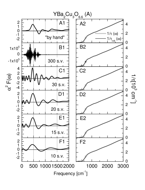
Figure 1: Spectral function $\alpha^{2}$F($\omega$) for underdoped YBa₂Cu₃O_6.6 with T_c= 59 K. The left panels show $\alpha^{2}$F($\omega$) and the right panels the experimental 1/$\tau(\omega)$ along with 1/$\tau_{cal}(\omega)$ calculated from the corresponding spectral function (Eq. (4)). The top panel shows previously published spectral function carbotte99 obtained from the scattering rate smoothed “by hand”. The other five pairs of panels are the data obtained using inverse theory. Different number of singular values are kept in the calculations, which results in different levels of smoothing. Note that the vertical scale in panels B1 and C1 is different.

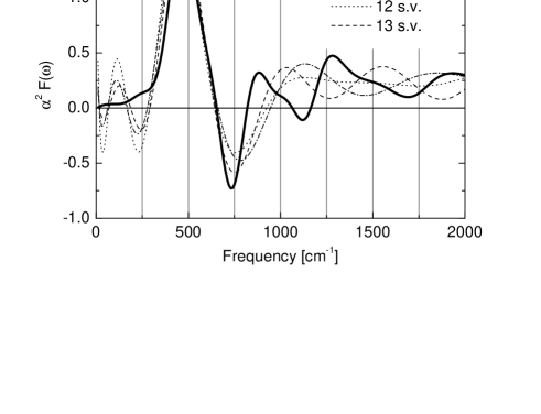
Figure 2: Spectral function $\alpha^{2}$F($\omega$) for underdoped YBa₂Cu₃O_6.6 with T_c= 59 K obtained by smoothing the experimental 1/$\tau(\omega)$ data “by hand” carbotte99 and with SVD with 11, 12 and 13 s.v.

The $\alpha^{2}$F($\omega$) spectra (Fig. 2) display characteristic shape with a strong peak at 480 cm^-1, followed by a strong dip at around 750 cm^-1. In addition there is weaker structure at both lower and higher frequencies. Carbotte et al. carbotte99 argued that the main peak is due to coupling of charge carriers to a collective bosonic mode and that it occurs at the frequency $\Delta+\omega_{s}$, where $\Delta$ is the maximum gap in the density of states and $\omega_{s}$ is the frequency of bosonic mode. They also claimed that in optimally doped Y123 the spectral weight of the peak matches that of neutron ($\pi$,$\pi$) resonance and is sufficient to explain high transition temperature in the cuprates. On the other hand Abanov et al. abanov01 argued that the main peak due to coupling to collective mode should be at 2$\Delta+\omega_{s}$. Moreover they argued that the fine structure at higher frequencies in $\alpha^{2}$F($\omega$) has physical significance: the second dip above the main peak should be at $\omega$= 4$\Delta$ and the next peak at $\omega$= 2$\Delta$+2$\omega_{s}$.

From Figs. 1 and 2 we conclude that extreme caution is required when performing numerical procedures based on the data smoothed “by hand”. In Fig. 2 the strongest peak at around 480 cm^-1 is fairly robust, although its spectral weight does change a few percent. However the other structures are very dependent on smoothing. The strongest dip shifts from 780 cm^-1 with 11 s.v., to 760 cm^-1 with 12 s.v. and 750 cm^-1 with 13 s.v. In the data smoothed “by hand” it is at 730 cm^-1. The spectral weight of the dip also varies. It was suggested by Abanov et al. abanov01 that the main dip, not the peak, is a better measure of the frequency 2$\Delta+\omega_{s}$. However based on our calculations (Fig. 2) the dip is even more sensitive to smoothing then the peak. Other peaks and dips do not display any correlation with the number of s.v., i.e. the level of smoothing.

IV Model calculations

The question we must now try to answer is how many s.v. to keep in inversion calculations. To address this issue we have performed calculations based on model spectral function with two Lorentzians:

$$\alpha^{2}F(\omega) = \frac{\omega_{p,a}^{2}\omega^{2}}{(\omega_{a}^{2}-\omega^{2})^{2}+(\gamma_{a}\omega)^{2}}+$$ (10)

$$\frac{\omega_{p,b}^{2}\omega^{2}}{(\omega_{b}^{2}-\omega^{2})^{2}+(\gamma_{b}\omega)^{2}},$$

with $\omega_{p,a}^{2}$= 50,000 cm^-1, $\omega_{a}$= 500 cm^-1, $\gamma_{a}$= 200 cm^-1, $\omega_{p,a}^{2}$= 250,000 cm^-1, $\omega_{a}$= 2,000 cm^-1 and $\gamma_{a}$= 800 cm^-1. This analytic form was chosen to mimic the “real” spectral function in cuprates (see for example Fig. (6) below). From this $\alpha^{2}$F($\omega$) the scattering rate was calculated (not shown) using Eq. (4) and then the formalism of inverse theory (Section II) was applied. Figure 3 shows the model spectral function (gray lines) along with the spectral function determined using inverse theory (black lines). We see that the “exact” solution (with all 300 s.v.) does not agree well with the model; this is due to numerical instabilities induced by smallest s.v. As we reduce the number of s.v. (cut-off the smallest) the agreement improves and for 100 and 50 s.v. the inversion reproduces the original spectral function. As we reduce the number of s.v. further the agreement begins to deteriorate and negative values in $\alpha^{2}$F($\omega$) appear again. Obviously these negative values are not real and simply reflect the fact that too few s.v. do not contain enough information to reproduce the original data. Note however that even with very few s.v. the main features of the spectral function are reproduced, as the main peaks and dips are roughly at correct frequencies (see for example calculations with 20, 15 and 10 s.v.). Their spectral weights are not reproduced though.

The optimal number of s.v. is always a trade–off between numerical precision and closeness to the data. Unfortunately, unlike model calculation shown in Fig. 3, in calculations with real data those two criteria are not well separated. Therefore one must be very careful when quantitatively analyzing the fine structure and their spectral weight in $\alpha^{2}$F($\omega$), as different levels and/or methods of smoothing can cause spurious shifts of the peaks and/or redistribution of their weights. For example visual inspection of 1/$\tau_{cal}(\omega)$ on the righthand side of Fig. 1 cannot distinguish between different levels of smoothing [compare 1/$\tau_{cal}(\omega)$ in panels C2, D2 or E2], however even the smallest differences manifest themselves in the spectral functions in the left panels.

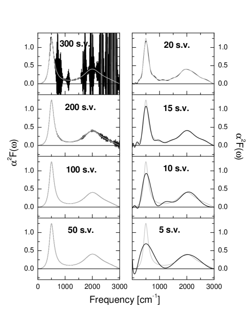
Figure 3: Model calculations of spectral function with two Lorentzians (Eq. 10). The “exact” solution, with all 300 s.v., does not agree well with the model because small singular values produce numerical instabilities in the solution. On the other hand if too few s.v. are kept unphysical negative regions appear. The model spectral function is recovered with 50–100 s.v.

An advantage of using inverse theory for extracting $\alpha^{2}$F($\omega$) is that we can quantify the smoothing procedure by specifying the number of s.v. different from zero in Eq. (9), thus eliminating arbitrariness related with smoothing of experimental data “by hand”. This is especially important when quantitatively comparing results from two different 1/$\tau(\omega)$ curves. Note however that if the data sets have different signal-to-noise levels, keeping the same number of s.v. will result in different levels of smoothing. We will encounter this problem below when we study doping dependence of $\alpha^{2}$F($\omega$) in Y123, since available data are from different sources.

Similar problems arise when analyzing temperature dependence of the data. Keeping the same number of singular values is again not the best way to achieve similar levels of smoothing. Fig. 4A shows the absolute values of first (biggest) 200 s.v. at different temperatures. They drop quickly (note the $\log$ scale) and such small $w_{i}$ produce large oscillations in the solution. To avoid that one cuts–off, i.e. replaces 1/$w_{i}$ with zeros in Eq. (9). As Fig. 4A shows s.v. are also very temperature dependent, and there are different ways to make the cut. As mentioned above keeping the same number of s.v. different from zero (“vertical cut”) is not a good way, as that would imply including smaller s.v. at higher temperatures and therefore higher frequency components into the solution. In such cases it is better to make “horizontal cuts”, i.e. keep the s.v. in the same range of absolute values. This implies different number of s.v. at different temperatures, but the oscillations in all the solutions should be approximately the same.

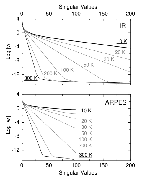
Figure 4: Singular values at different temperatures. Top panel: first (biggest) 200 s.v. from IR; bottom panel: all 100 s.v. from ARPES. When analyzing temperature dependence of the spectral function “horizontal cuts” are more appropriate, assuming all data sets have the same signal-to-noise ratio. On the other hand for doping dependence studies (at the same temperature) “vertical cuts”, i.e. the same number of s.v., should produce similar levels of smoothing.

V Problem of negative values

An obvious problem with these (Figs. 1 and 2) and previous (Ref. carbotte99, ; schachinger00, ; schachinger01, ; wang01, ; abanov01, ; singley01, ; tu02, ) calculations is that they all produce non-physical negative values in the spectral function. The latter function is proportional to boson density of states F($\omega$) and therefore cannot be negative. The important issue we must address is the origin of these negative values. As shown in Fig. 3 negative values can appear because of numerical problems: either because small s.v. produce numerical instabilities, or because too few s.v. do not contain sufficient information to reproduce the original data. These negative values are not real and can be eliminated either by choosing appropriate number of s.v., or by some other numerical technique, as we will show below.

However, negative values can also have a real physical origin, and they cannot be eliminated by any numerical procedure. Namely, all the methods we have discussed (Eqs. (1), (3) or (4)) were developed for normal state, but are frequently used in the (pseudo)gapped state abanov01 ; comm-varma . In order to illustrate the insufficiency of these models to account for a (pseudo)gap in the density of states we have performed inversion calculations on BCS scattering rate. Fig. 5 shows that scattering rate (right panels) calculated within BCS with $\Gamma$= 2$\Delta$= 400 cm^-1, at T/T_c= 0.1. The spectral functions calculated with different number of s.v., i.e. different levels of smoothing are shown in left panels. Surprisingly they look very similar to those produced by coupling of carriers to collective bosonic mode (see Figs. 1 and 2): there is a strong peak roughly at the frequency of the gap, followed by a strong dip and fine structure which is smoothing dependent.

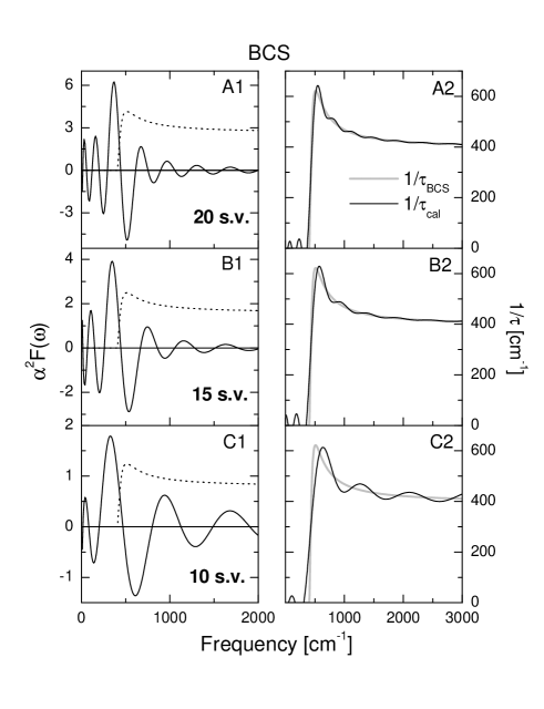
Figure 5: Model calculations of spectral function from BCS scattering rate. Left panels display calculated spectral function $\alpha^{2}$F($\omega$) and the right panels the BCS scattering rate (also shown with dotted lines in left panels) and 1/$\tau_{cal}(\omega)$ calculated from the spectral function on the left. A gap in the density of states produces similar structure in $\alpha^{2}$F($\omega$) as does the coupling to a bosonic mode.

The main issue now is whether one can distinguish between real, physical negative values arising because of the gap in the density of states and those arising because of numerical instabilities. Using inverse theory we can also address this problem. A so called deterministic constraints nr can be imposed on the solution during the inversion process. These deterministic constraints reduce the set of possible solutions from which the “best” solution will be picked. In the case of spectral function an obvious constrain is $\alpha^{2}$F($\omega$)$\geq$ 0 for all $\omega$. However other constraints are also possible. In fact one of them, that $\alpha^{2}$F($\omega$)= 0 above some cut-off frequency (3,000 cm^-1), was implicitly assumed in all previous calculations, as the limits in the integral in Eq. (4) run from zero to infinity, and the sum in Eq. (6) runs only up to 3,000 cm^-1.

Numerically one applies the constraints during an iterative inversion process nr . The initial solution $\vec{a}_{0}$ for the iteration can be obtained either from Eq. (7) or more generally using a so called regularization:

$$K^{T}\vec{\gamma}=(K^{T}K+\delta H)\vec{a},$$ (11)

where $H$ is a so called regularization matrix and $\delta$ is a regularization parameter. For $\delta$=0 (no regularization) Eq. (11) reduces to Eq. (7). Eq. (11) can also be solved using SVD. Once the initial solution $\vec{a}_{0}$ is found, one applies iteration, imposing the constraint $\alpha^{2}$F($\omega$)$\geq$ 0 in every step:

$$\vec{a}_{n+1}=P[(I-\beta\delta H)\vec{a}_{n}+\beta K^{T}(\vec{\gamma}-H\vec{a}_{n})],$$ (12)

where $\beta$ is the iteration parameter and $P$ denotes an operator that sets all the negative values in the solution to zero. The results of these calculations for YBa₂Cu₃O_6.6 with T_c= 59 K are shown in Fig. 6. The initial solution (top panels) was obtained from SVD with 20 s.v. and no regularization. This solution was then iterated different number of times: 100 (panel B), 200 (C), 500 (D) and 1000 (F). For each intermediate solution the scattering rate 1/$\tau_{cal}(\omega)$ (gray lines) was calculated using Eq. (4).

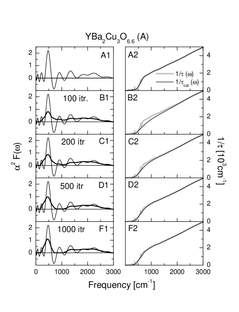
Figure 6: Spectral function $\alpha^{2}$F($\omega$) for underdoped YBa₂Cu₃O_6.6 with T_c= 59 K. A deterministic constraint $\alpha^{2}$F($\omega$)$\geq$ 0 is applied iteratively (Eq. (12)). The top two panels show the initial solution with 20 s.v. The other four sets of panels display intermediate solutions for several different levels of iterations.

Clearly as the number of iterations increase the agreement between 1/$\tau(\omega)$ and 1/$\tau_{cal}(\omega)$ becomes better, but it never becomes as good as the one with negative values (top panel). It appears that the numerical process converges, although very slowly, to the solution with negative values: some frequency regions in $\alpha^{2}$F($\omega$) have simply been cut–off by the program. The position of the main peak is not affected, but its intensity has been reduced significantly. We also emphasize that the structure in the spectral function at $\omega>$ 1,000 cm^-1 is essential for obtaining linear frequency dependence of 1/$\tau(\omega)$ up to very high frequencies. We will return to this important issue in Section IX below.

Therefore in the case of YBa₂Cu₃O_6.60 we have been able to eliminate negative values and at least in principle obtain $\alpha^{2}$F($\omega$) which is always positive. This indicates that the structure in the spectral function is (predominantly) due to coupling to bosonic mode and not the gap in the density of states. On the other hand, we have not been able to obtain good BCS scattering rate without negative values in spectral function (not shown). This is not unexpected as the form of spectral function is entirely due to a gap in the density of states (no bosonic mode), which Eqs. (1) and (4) do not take into account. We have encountered similar situation in some cuprates. Fig. 7 displays inversion calculations for several Y123 samples with different doping levels and/or T_c: YBa₂Cu₃O_6.60 with T_c = 57 K (Ref. homes99, ), YBa₂Cu₃O_6.60 with T_c = 59 K (Ref. carbotte99, ) and YBa₂Cu₃O_6.95 with T_c = 91 K (Ref. homes99, ). All calculations are for T= 10 K, with a fixed number of 15 s.v. As can be seen from Fig. 7 the peak systematically shifts to higher energies as doping and T_c increase: 430 cm^-1 in x=6.6 with T_c= 57 K, 480 cm^-1 in the second x=6.6 with T_c= 59 K and 520 cm^-1 in x=6.95. For both 6.6 samples we have been able to obtain relatively good inversions (dashed lines) without negative values in the spectral function. That is not the case for 6.95 sample where without negative values the inversion fails badly (see dashed line in the bottom–right panel). This indicates that the form of scattering rate is probably a combination of coupling to collective mode and a gap in the density of states, as pointed out by Timusk timusk03 .

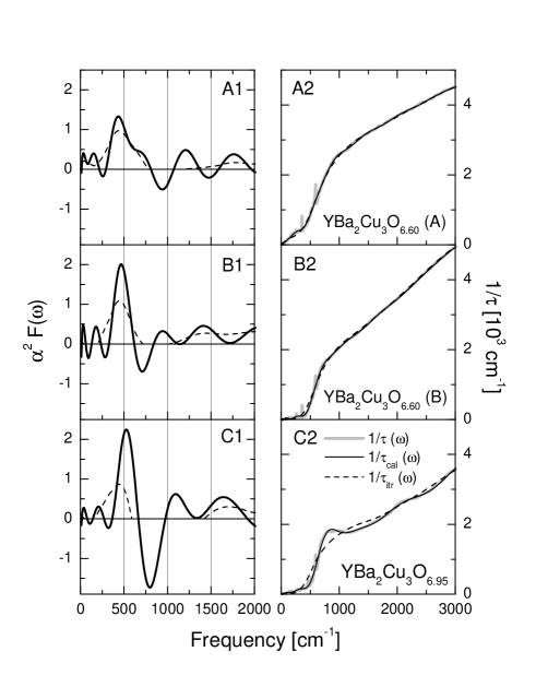
Figure 7: Doping dependence of spectral function $\alpha^{2}$F($\omega$) for (A) YBa₂Cu₃O_6.60 with T_c = 57 K (Ref. homes99, ), (B) YBa₂Cu₃O_6.60 with T_c = 59 K (Ref. carbotte99, ) and (C) YBa₂Cu₃O_6.95 with T_c = 91 K (Ref. homes99, ). All curves are for the lowest measured temperature T$\approx$ 10 K. “Vertical cuts”, i.e. the same number of singular values (15), were made for all three data sets. Left panels display 1/$\tau(\omega)$ data along with 1/$\tau_{cal}(\omega)$. Dashed lines are the results of iterative calculations. Relatively good fits without negative values in $\alpha^{2}$F($\omega$) can be obtained for both YBa₂Cu₃O_6.60 samples, but not for YBa₂Cu₃O_6.95.

VI Electron-boson coupling vs. energy gap

As demonstrated in previous sections similar shapes of $\alpha^{2}F(\omega)$ are produced by coupling to bosonic mode and a gap in the density of states when equations for the normal state (Eq. (1) or (4)) are used. It is essential to discriminate these two contribution because they usually appear together. To address this problem we have to apply Allen’s formula for the scattering rate in the superconducting state allen71 :

$$\frac{1}{\tau(\omega)}=\frac{2\pi}{\omega}\int_{0}^{\omega-2\Delta}d\Omega(\omega-\Omega)\alpha^{2}F(\Omega)E\Big{[}\sqrt{1-\frac{4\Delta^{2}}{(\omega-\Omega)^{2}}}\Big{]}$$ (13)

In this equation $E(x)$ is the complete elliptic integral of the second kind and $\Delta$ is a gap in the density of states. For $\Delta$=0 Eq. (13) reduces to Eq. (1) for the normal state. Numerically Eq. (13) is again Fredholm integral equation of the second kind and the same numerical procedure for its solution can be used.

We have performed inversion of the data for optimally doped YBa₂Cu₃O_6.95 using Eq. (13). Fig. 8 shows inversion calculations for different values of the gap $\Delta$. The top panels display calculations with $\Delta$=0, which is equivalent to previous calculations using Eq. (4) (Fig. 7). As we already discussed it, the spectrum is dominated by a pronounced peak, followed by a large negative deep. Unlike YBa₂Cu₃O_6.6 for which this negative deep can, at least in principle, be eliminated, the deep in YBa₂Cu₃O_6.95 cannot be eliminated (Fig. 7) and in the previous section we suggested that that is because of the gap. Indeed when finite values of the gap are used in Eq. (13) this negative deep following the main peak is strongly suppressed; calculated spectral function positive for almost all frequencies (Fig. 8).

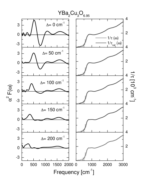
Figure 8: Spectral function $\alpha^{2}$F($\omega$) for optimally doped YBa₂Cu₃O_6.95 calculated from Eq. (13) for the scattering rate in the superconducting state. Different values of the gap $\Delta$=0–200 cm^-1 were used in the calculations. For $\Delta$=0 there is a pronounced deep following the main peak. However when finite values of the gap are introduced the negative deep gradually disappears and the main peak shifts to lower energies.

The problem with Eq. (13) is that it is based on s-wave energy gap at T= 0 K. These two assumptions imply that the scattering rate must be zero below 2$\Delta$, which is never the case with cuprates because of the d-wave gap and because the data was taken at finite temperature. In spite of this, Eq. (13) is useful because it can provide some insight into charge dynamics in cuprates. Fig. 9 displays calculations of scattering rate based on model spectral function $\alpha^{2}$F($\omega$) shown with thin line. When the gap is zero the data qualitatively looks like underdoped YBa₂Cu₃O_6.6: at higher frequencies it is linear and it is suppressed below certain energy (black line). However for the finite values of the gap ($\Delta$=200 cm^-1) the data looks more like optimal YBa₂Cu₃O_6.95: there is overshoot just above the suppressed region (gray line).

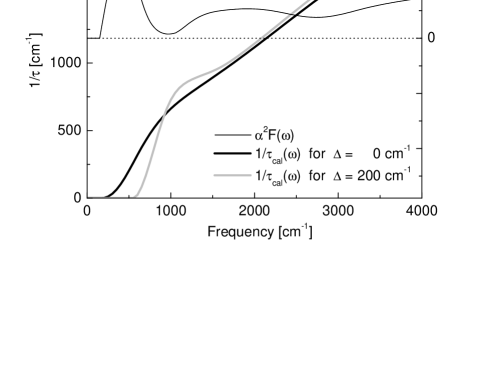
Figure 9: Model spectral function $\alpha^{2}$F($\omega$) (thin line) is used to calculate the scattering rate 1/$\tau_{cal}(\omega)$ from Eq. (13). For $\Delta$=0 calculated scattering rate resembles 1/$\tau(\omega)$ of underdoped YBa₂Cu₃O_6.60 (Fig. 7). However for finite values of the gap calculated scattering rate resembles 1/$\tau(\omega)$ of optimally doped YBa₂Cu₃O_6.95: there is an overshoot following the suppressed region (Fig. 7).

Based on these model calculations it appears that the response of YBCO on the underdopd side is dominated by coupling to bosonic mode, whereas at optimal doping the gap plays more prominent role. Indeed recent ARPES and tunneling measurements have shown that the Fermi surface of cupares is continuously destroyed with underdoping norman98 ; mcelroy04 . On the underdoped side antinodal states do not exist (they are incoherent) and the IR response is dominated by nodal states which are coherent and not gaped. On the other hand the IR response at optimal doping is more complicated, because both antinodal (gaped) and nodal (not gaped) states are coherent and contribute to the IR response.

VII Electron–boson spectral function of Bi2212

In this section we analyze the temperature dependence of the spectral function for optimally doped Bi2212 with T_c=91 K. The same data set has been analyzed before tu02 using Eq. (3). The calculated spectra (Fig. 10) look qualitatively similar to those obtained on Y123 (Fig. 2), with a strong peak in the far-IR range followed by a dip, and high frequency contribution that extends up to several thousand cm^-1. To achieve similar levels of smoothing at different temperatures “horizontal cut” has been made (Fig. 4A).

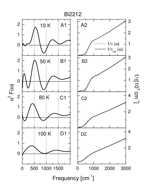
Figure 10: Temperature dependence of the spectral function $\alpha^{2}$F($\omega$) for optimally doped Bi₂Sr₂CaCu₂O_8-δ with T_c= 91 K. As temperature increases the main peak shifts to lower energies and looses intensity, but seems to persist even above T_c.

In the normal state at T=100 K we identify a peak at $\approx$ 400 cm^-1 (50 meV). Note that the peak is at somewhat lower energy then in Ref. tu02, , which can be traced back to the use of Eq. (3), which is strictly speaking valid only at T=0 K. We also note that the peak is observed above T_c, unlike the ($\pi$, $\pi$) resonance detected in INS only in the superconducting state fong99 .

As temperature decreases below T_c the peak shifts to higher energies: 430 cm^-1 at 80 K, 520 cm^-1 at 50 K and 560 cm^-1 at 10 K. At the lowest temperature the spectral function is almost identical to previously reported tu02 , which confirms that at 10 K Eqs. (3) and (4) are equivalent. According to theoretical considerations carbotte99 ; abanov01 in the superconducting state the peak should be off-set from the resonance frequency of the ($\pi$, $\pi$) peak ($\omega_{s}\simeq$ 43 meV) by one or two gap values ($\Delta$=34 meV, Ref. rubhausen98, ). At 10 K the peak is at 70 meV, somewhat lower than $\Delta+\omega_{s}$= 77 meV (Ref. carbotte99, ) and significantly lower than 2$\Delta+\omega_{s}$= 111 meV (Ref. abanov01, ). This result is in contrast with optimally doped Y123 where the IR peak at 66 meV (Fig. 7) is in relatively good agreement with $\Delta+\omega_{s}$=27 meV+41 meV= 68 meV Ref. carbotte99, .

VIII Inversion of ARPES data

Recently it has been argued based on ARPES data bogdanov00 ; lanzara01 ; shen03 ; zhou03 that in cuprates electrons are strongly coupled to phonons and that such strong coupling might be responsible for high T_c. In light of these suggestions there have been several attempts to determine $\alpha^{2}$F($\omega$) from ARPES data verga02 ; schachinger03 ; shi04 . Inversion by Verga et al. verga02 was based on the imaginary part of the self-energy $\Sigma_{2}(\omega)$, obtained from the real part $\Sigma_{1}(\omega)$ through Kramers–Kronig transformation. The spectral function was then calculated by differentiation of $\Sigma_{2}(\omega)$, a procedure which necessarily requires smoothing “by hand”. On the other hand Schachinger et al. schachinger03 have modeled the spectral function with analytical functions and then used these models to simultaneously fit both the IR and ARPES spectra. Maximum Entropy Method (MEM) has recently been used to invert ARPES data and obtain $\alpha^{2}$F($\omega$) for beryllium surface Be(10$\overline{1}$0) (Ref. shi04, ) and LSCO (Ref. zhou04, ). Here we apply the same inversion method we used for IR to ARPES. The procedure of extracting $\alpha^{2}$F($\omega$) is based on standard expression for the real part of quasiparticle self-energy $\Sigma_{1}(\omega)$ (Ref. allen82, ):

$$\Sigma_{1}(\omega) = \int_{0}^{\infty}d\Omega\alpha^{2}F(\Omega)\cdot$$ (14)

$$\Re\Big{[}\Psi\Big{(}\frac{1}{2}+i\frac{\Omega-\omega}{2\pi T}\Big{)}-\Psi\Big{(}\frac{1}{2}-i\frac{\Omega+\omega}{2\pi T}\Big{)}\Big{]},$$

where $\Psi(x)$ is digamma function. The real part of the self-energy $\Sigma_{1}(E_{k})$ can be obtained from ARPES data as allen82 :

$$\Sigma_{1}(E_{k})=E_{k}-\epsilon_{k},$$ (15)

where E_k is the renormalized dispersion measured in ARPES experiments and $\epsilon_{k}$ is the bare electron dispersion. As the latter function is not independently known, a common procedure when using Eq. (15) is to assume a linear bare dispersion ($\epsilon_{k}\sim k$) and no renormalization at higher energies, i.e. E_k=$\epsilon_{k}$ above $\approx$ 250 meV. Expression (14) is again a Fredholm integral equation of the first kind and the same numerical technique described in Section II can be used for its solution. Similar to IR, “by hand” smoothing of the data is not needed, as SVD procedure will allow us to smooth the solution by reducing the number of non-zero s.v. Since the resolution of ARPES data is poorer than IR, in all calculations we used vectors and matrices with dimensions 100 instead of 300.

As an example of this procedure in Figure 11 we first present spectral function $\alpha^{2}$F($\omega$) calculated from ARPES data for molybdenum surface Mo(110) (Ref. valla99, ). As before, left panels show the calculated spectral function and right panels measured ARPES dispersion E_k and dispersion calculated from Eq. (14) E_k,cal using the corresponding spectral function on the left. The spectral function has a characteristic shape, with a strong peak at around 200 cm^-1 and weaker structure at both higher and lower frequencies. Similar to IR, position of the main peak is fairly robust against smoothing, but weaker peaks and dips are not. The dashed lines in the left-hand panels represent $\alpha^{2}$F($\omega$) calculated based on band structure savrasov96 . Low data resolution and loss of information during the inversion do not allow us to resolve the fine structure in $\alpha^{2}$F($\omega$) that has been predicted numerically savrasov96 . At higher energies ($\omega\gtrsim$ 400 cm^-1) the spectral function is effectively zero, in accord with band structure calculations.

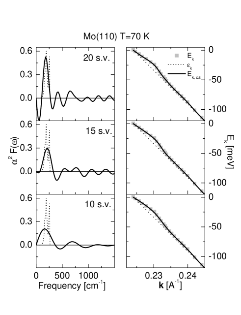
Figure 11: Spectral function $\alpha^{2}$F($\omega$) of Mo(110) surface at 70 K extracted from ARPES data valla99 . Three different levels of smoothing are shown with 10, 15 and 20 s.v. Dotted lines in left panels represent theoretical spectral function savrasov96 .

These relatively simple calculations for molybdenum surface Mo(110) have uncovered the limitations of inversion of ARPES data. Fine details of the spectral function, especially narrow peaks, cannot be resolved as they are convoluted in the experimental data (Eq (14)). Maximum information that can be obtained is the frequency region where there is significant contribution to $\alpha^{2}$F($\omega$). It has recently been claimed based on MEM inversion of ARPES data that the sharp peaks identified in $\alpha^{2}$F($\omega$) spectra are due to specific phonon modes shi04 ; zhou04 . Based on our calculations we speculate that it is unlikely that such fine details of the spectra could be resolved by any inversion procedure.

Figure 12 presents the data for optimally doped Bi2212 (T_c= 91 K) at 130 K and 70 K taken along nodal direction. Similar to IR calculations in Fig. 10, to achieve approximately the same level of smoothing different number of s.v. values were kept in calculations at different temperatures: 8 (out of 100) at 130 K and 10 at 70 K. Within the error bars the main peak does not shift with temperature: it is at 440 cm^-1 at both 130 K and 70 K. However the peak does narrow and gains strength at 70 K (Ref. arpes-sv, ). Below 70 K ARPES dispersion displays almost no temperature dependence. Note also that unlike IR, there seems to be less problems with negative values in ARPES $\alpha^{2}$F($\omega$) calculations. In particular there is no pronounced dip following the main peak, which might be related to the fact that the APRES scans were taken along ($\pi$, $\pi$) direction where the magnitude of the gap goes to zero. Another important difference compared with IR is that there is no high frequency component in ARPES: the whole contribution to $\alpha^{2}$F($\omega$) is concentrated at $\omega\lesssim$ 750 cm^-1.

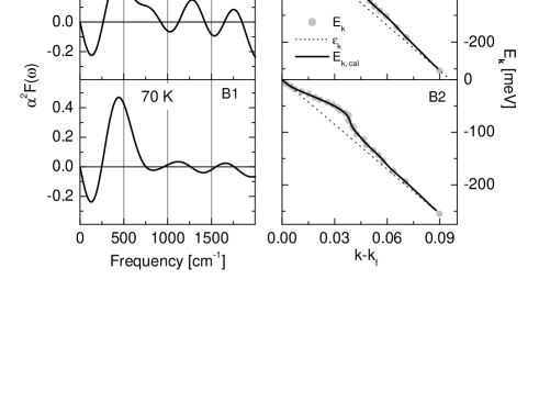
Figure 12: Temperature dependence of spectral function $\alpha^{2}$F($\omega$) of optimally doped Bi2212 extracted from ARPES data (along nodal direction) using inverse theory. Left panels show $\alpha^{2}$F($\omega$) spectra calculated from Eq. (14), and right panels ARPES quasiparticle dispersion E_k (gray symbols) and calculated dispersion E_k,cal (full lines) using corresponding spectral function on the left. Also shown with dashed lines are bare quasiparticle dispersions $\epsilon_{k}$ used to calculate $\Sigma_{1}(\omega)$ (Eq. (15)).

IX IR–ARPES comparison

In the previous section the inversion calculations have uncovered several important differences between the spectral function extracted from IR and ARPES. In all ARPES calculations the strong dip following the main peak was absent, which we suggested was due to the absence of the gap along the ($\pi$, $\pi$) symmetry direction. More importantly, there was no high frequency contribution extending up to several thousand cm^-1 in any ARPES calculations. In this section we will make an explicit comparison between IR and ARPES spectral functions and discuss their similarities and differences.

First it should be emphasized that ARPES $\alpha^{2}$F($\omega$) from Eq. (14) is not the same as the IR from Eqs. (1) and (4) allen82 ; schachinger03 . ARPES is a momentum resolving technique, whereas IR averages over the Brillouin zone. More importantly ARPES probes the equilibrium $\alpha^{2}$F($\omega$) (single-particle property), whereas IR measures transport $\alpha_{tr}^{2}$F($\omega$) (two-particle property) allen82 . Recently Schachinger, et al. discussed the difference schachinger03 and suggested that in the simplest case these two functions might differ only by a numerical factor of 2–3. Therefore it would be very instructive to directly compare the spectral functions extracted from IR and ARPES. However technical reasons make this comparison difficult. Present resolution of ARPES data of $\approx$ 10 meV is at least one order of magnitude less than IR (typically $\lesssim$ 1 meV in the frequency range of interest). This large discrepancy in resolution requires different levels of smoothing, which can affect the solution. Therefore we cautiously compare calculated $\alpha^{2}$F($\omega$)’s, relying only on robust features, as discussed in the previous sections.

The most complete comparison can be made for optimally doped Bi2212, for which high quality IR tu02 and ARPES fedorov99 data sets exist, all obtained on the samples from the same batch gu90 . Although data at different temperatures are available, we believe that will not change the main results and conclusions in any significant way, as ARPES data display little temperature dependence below 70 K (Ref fedorov99, ). Fig. 13 shows $\alpha^{2}$F($\omega$) from both IR and ARPES for optimally doped Bi2212 with T_c= 91 K. The $\alpha^{2}$F($\omega$) from ARPES is multiplied by a factor of 3. The agreement between the positions of the main peak in both data sets ($\approx$ 500 cm^-1) is very good. This agreement is actually surprising and unexpected. As discussed in Sections III and VII the main peak in IR spectral function should be off-set from the frequency of the neutron peak $\omega_{s}$ by either one carbotte99 or two abanov01 gap values $\Delta$. On the other hand in ARPES data the gap should not play a role: the data were taken along the nodal directions where the gap is zero. Therefore almost perfect agreement between the positions of IR and ARPES peaks (and disagreement with INS peak - see Section VII) in optimally doped Bi2212 is puzzling and calls for further theoretical studies.

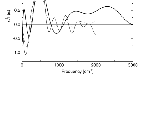
Figure 13: Comparison of spectral functions $\alpha^{2}$F($\omega$) extracted from IR and ARPES data for optimally doped Bi2212 with T_c= 91 K. Note that $\alpha^{2}$F($\omega$) from ARPES is multiplied by a factor of three. Dashed line is an ARPES calculation with a different bare dispersion (with renormalization effects up to 0.5 eV).

Another important difference between IR and ARPES is the contribution in IR that extends up to very high energies. There is no such contribution in any ARPES data we have available (Section VIII). Therefore based on ARPES data alone one can argue that the observed contribution to $\alpha^{2}$F($\omega$) is either due to phonons or spin fluctuations. On the other hand the high frequency component in always present in IR and is necessary to keep 1/$\tau(\omega)$ increasing, approximately linearly with $\omega$. Figure 14 displays calculations of $\alpha^{2}$F($\omega$) for YBa₂Cu₃O_6.6 with T_c= 59 K up to almost 1 eV (Ref. carbotte99, ). Both inversion with negative values (top panels) and iterative calculations with positive values (middle panels) result in spectral function with significant contributions up to $\approx$ 0.85 eV. If this contribution is cut off, for example at 1,000 cm^-1 (bottom panels), calculated scattering rate deviates strongly from experimental data, as 1/$\tau_{cal}(\omega)$ tends to saturate above $\sim$ 2,000 cm^-1. This result argues against phonons as the origin of the structure in $\alpha^{2}$F($\omega$), as phonon spectrum cannot extend up to such high frequencies. However phonon contribution below $\approx$ 1,000 cm^-1 cannot be ruled out.

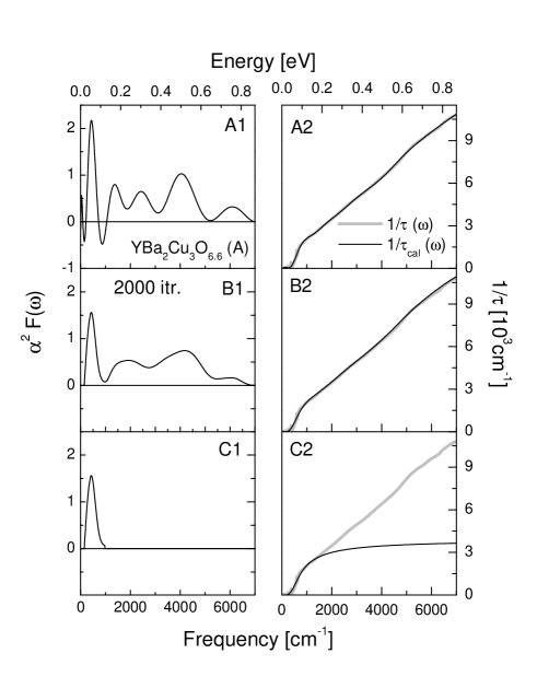
Figure 14: Spectral function $\alpha^{2}$F($\omega$) extracted from IR data for underdoped YBa₂Cu₃O_6.6 with T_c= 59 K and calculated up to $\approx$ 0.85 eV. Top panels display calculations with negative values (Section II). Middle panels are iterative calculations with 2,000 iterations (Section V). In both cases significant contribution to $\alpha^{2}$F($\omega$) persist up to very high frequencies. Bottom panels display the result of calculation of 1/$\tau_{cal}(\omega)$ with high frequency contribution to $\alpha^{2}$F($\omega$) cut-off (above 1,000 cm^-1). In this case the calculated scattering rate tends to saturate at higher energies.

The absence of high-frequency contribution in ARPES is puzzling and seems to indicate that the difference between IR and ARPES spectral function might be more than just a numerical prefactor. On the other hand it may also signal intrinsic problems with our procedure of extracting $\Sigma_{1}(E_{k})$ from ARPES dispersion kordyuk04 . As mentioned in Section VIII, bare electron dispersion $\epsilon_{k}$ is not known and some assumptions must be made before Eq. (15) can be used. The most common assumptions are: 1) linear bare dispersion $\epsilon_{k}$ and 2) no renormalization above certain cut-off frequency. We have employed these assumptions in all our calculations, with a cut-off of typically $\approx$ 250 meV. The use of both of these assumptions in highly unconventional systems like cuprates is questionable and requires further theoretical treatment kordyuk04 .

In order to check the effect upper cut-off energy has on the solution we have performed $\alpha^{2}$F($\omega$) inversion for optimally doped Bi2212 (Fig. 12) assuming that the renormalization persist up to 0.5 eV, instead of 0.25 eV. Fig. 13 also shows this new calculation with dashed line and obviously there is very little difference: the main peak is in good agreement and there is no significant contribution above $\approx$ 800 cm^-1, even though the renormalization extends up to 0.5 eV. We speculate that in order to obtain spectral function similar to IR, either the renormalization must persist up to several eV or some more sophisticated form of the bare dispersion $\epsilon_{k}$ must be used kordyuk04 .

X Summary and Outlook

A new numerical procedure of extracting electron–boson spectral function from IR and ARPES data based on inverse theory has been presented. The new method eliminates the need for differentiation and smoothing “by hand”. However we also showed that the information is convoluted and fine details of $\alpha^{2}$F($\omega$) cannot be extracted, no matter what numerical technique one uses. This especially holds for ARPES, whose current data resolution is particularly poor compared to IR.

Using this new procedure we have extracted $\alpha^{2}$F($\omega$) from IR and/or ARPES data in a series of Y123 and Bi2212 samples. The calculations have uncovered several important differences between IR and ARPES spectral functions. All IR spectral functions contain, in addition to a strong peak at low frequencies ($\omega\lesssim$ 500 cm^-1), contributions that extend up to very high energies (typically several thousand cm^-1). On the other hand none of ARPES spectral functions display such high energy contribution. Therefore we concluded that based on ARPES results one cannot distinguish between phonon and magnetic scenarios, as the main peak in $\alpha^{2}$F($\omega$) can have either (or both) magnetic or phonon components. However in all IR results the observed high frequency contribution extends to much higher than typical phonon frequencies, the result which argues against phonon mechanism.

Finally, the observed differences between IR and ARPES have prompted us to speculate that $\alpha^{2}$F($\omega$) from these two experimental techniques might contain qualitatively different information. Alternatively, we suggest that the whole concept of coupling of charge carriers to collective boson modes in the cuprates needs to be revised.

- (1) J.P. Carobotte, Rev.Mod.Phys. 62, 1027 (1990).
- (2) W.L. McMillan and J.M. Rowell, Phys.Rev.Lett. 14, 108 (1965).
- (3) B. Farnworth and T. Timusk, Phys.Rev.B 10, 2799 (1974).
- (4) B. Farnworth and T. Timusk, Phys.Rev.B 14, 5119 (1976).
- (5) F. Marsiglio, T. Startseva and J.P. Carbotte, Physics Letters A 245, 172 (1998).
- (6) G.A. Thomas, J. Orenstein, D.H. Rapkine, M. Capizzi, A.J. Millis, R.N. Bhatt, L.F. Schneemeyer, and J.V. Waszczak, Phys.Rev.Lett. 61, 1313 (1988).
- (7) D. Pines, Physica B 163, 78 (1990).
- (8) J.P. Carbotte, E. Schachinger and D.N. Basov, Nature 401, 354 (1999).
- (9) D. Munzar, C. Bernhard and M. Cardona, Physica C 121, 121 (1999).
- (10) P. Bourges in The gap Symmetry and Fluctuations in High Temperature Superconductors, edited by J. Bok, G Deutscher, D. Pavuna and S.A. Wolf. (Plenum Press, 1998), and references therein.
- (11) Pengcheng Dai, H.A. Mook, R.D. Hunt and F. Dogan, Phys.Rev.B 63, 054525 (2001), and references therein.
- (12) P.V. Bogdanov, A. Lanzara, S.A. Kellar, X.J. Zhou, E.D. Lu, W.J. Zheng, G. Gu, J.-I. Shimoyama, K. Kishio, H. Ikeda, R. Yoshizaki, Z. Hussain and Z.X. Shen, Phys.Rev.Lett. 85, 2581 (2000).
- (13) A. Lanzara, P.V. Bogdanov, X.J. Zhou, S.A. Kellar, D.L. Feng, E.D. Lu, T. Yoshida, H. Eisaki, A. Fujimori, K. Kishio, J.-I. Shimoyama, T. Noda, S. Uchida, Z. Hussain, Z.-X. Shen, Nature 412, 510 (2001).
- (14) Z.-X. Shen, cond-mat/0305576.
- (15) X.J. Zhou, T. Yoshida, A. Lanzara, P.V. Bogdanov, S.A. Kellar, K.M. Shen, W.L. Yang, F. Ronning, T. Sasagawa, T. Kakeshita, T. Noda, H. Eisaki, S. Uchida, C.T. Lin, F. Zhou, J.W. Xiong, W.X. Ti, Z.X. Zhao, A. Fujimori, Z. Hussain, and Z.-X. Shen, Nature 423, 398 (2003).
- (16) Attempts of using inverse theory have been reported timusk76 ; shulga01 ; shi04 .
- (17) S.V. Shulga, cond-mat/0101243.
- (18) Junren Shi, S.-J Tang, Biao Wu, P.T. Sprunger, W.L. Yang, V. Brouet, X.J. Zhou, Z. Hussain, Z.-X. Shen, Zhenyu Zhang, E.W. Plummer, Phys.Rev.Lett. 92, 186401 (2004).
- (19) P.B. Allen, Phys.Rev.B 3, 305 (1971).
- (20) A.V. Puchkov, D.N. Basov and T. Timusk, J.Phys C 8, 10049 (1996).
- (21) E. Schachinger and J.P. Carbotte, Phys.Rev.B 62, 9054 (2000).
- (22) E. Schachinger, J.P. Carbotte and D.N. Basov, Europhys.Lett. 54, 380 (2001).
- (23) N.L. Wang and B.P. Clayman, Phys.Rev.B 63, 052509 (2001).
- (24) A. Abanov, A.V. Chubukov and J. Schmalian, Phys.Rev.B 63, 180510(R) (2001).
- (25) E.J. Singley, D.N. Basov, K. Kurahashi, T. Uefuji and K. Yamada, Phys.Rev.B 64, 224503 (2001).
- (26) J.J. Tu, C.C. Homes, G.D. Gu, D.N. Basov and M. Strongin, Phys.Rev.B 66, 144514 (2002).
- (27) N.L. Wang, P. Zheng, J.L. Luo, Z.J. Chen, S.L. Yan, L. Fang, Y.C. Ma, Phys.Rev.B 68, 054516 (2003).
- (28) S.V. Shulga, O.V. Dolgov and E.G. Maksimov, Physica C 178, 266 (1991).
- (29) Inverse theory can also be applied to Allen’s formula Eq. (1), but obviously the result will only be valid at T= 0 K.
- (30) W.H. Press, S.A. Teukolsky and W.T. Vetterling and B.P. Flannery, Numerical Recipes, Cambridge University Press (2002), and references therein.
- (31) In general, matrix K can be rectangular, i.e. vectors and do not have the same size nr . For simplicity in all our calculations we used quadratic matrices.
- (32) An exact numerical treatment has recently been proposed varma03 , but this is beyond the scope of our discussion.
- (33) I. Vekhter and C.M. Varma, Phys.Rev.Lett. 90, 237003 (2003).
- (34) C.C. Homes, D.A. Bonn, Ruixing Liang, W.N. Hardy, D.N. Basov, T. Timusk, B.P. Clayman, Phys.Rev.B 60, 9782 (1999).
- (35) T. Timusk, cond-mat/0303383.
- (36) M.R. Norman, H. Ding, M. Randeria, J.C. Campuzano, T. Yokoya, T. Takeuchi, T. Takahashi, T. Mochiku, K. Kadowaki, P. Guptasarma and D.G. Hinks, Nature 392, 157 (1998).
- (37) K. McElroy, D.-H. Lee, J.E. Hoffman, K.M. Lang, J. Lee, E.W. Hudson, H. Eisaki, S. Uchida and J.C. Davis, cond-mat/0406491.
- (38) S. Verga, A. Knigavko and F. Marsiglio, Phys.Rev.B 67, 054503 (2003).
- (39) E. Schachinger, J.J. Tu and J.P. Carbotte, Phys.Rev.B 67, 214508 (2003).
- (40) X.J. Zhou, Junren Shi, T. Yoshida, T. Cuk, W.L. Yang, V. Brouet, J. Nakamura, N. Mannella, Seiki Komiya, Yoichi Ando, F. Zhou, W.X. Ti, J.W. Xiong, Z.X. Zhao, T. Sasagawa, T. Kakeshita, H. Eisaki, S. Uchida, A. Fujimori, Zhenyu Zhang, E.W. Plummer, R.B. Laughlin, Z. Hussain and Z.-X. Shen, cond-mat/0405130.
- (41) P.B. Allen and B. Mitrovic, in Solid State Physics, edited by H. Ehrenreich, F. Seitz and D. Turnbull (Academic, New York, 1982) Vol.37, p.1.
- (42) T. Valla, A.V. Fedorov, P.D. Johnson and S.L. Hulbert, Phys.Rev.Lett. 83, 2085 (1999).
- (43) S.Y. Savrasov and D.Y. Savrasov, Phys.Rev.B 54, 16487 (1996).
- (44) A.V. Fedorov, T. Valla, P.D. Johnson, Q. Li, G.D. Gu and N. Koshizuka, Phys.Rev.Lett. 82 2179 (1999).
- (45) G. Gu, K. Takamku, N. Koshizuka and S. Tanaka, J.Cryst.Growth, 130, 325 (1993).
- (46) H.F. Fong, P. Bourges, Y. Sidis, J.P. Regnault, A. Ivanov, G.D.Gu, N. Koshizuka and B. Keimer, Nature 398, 588 (1999).
- (47) Fig. 4B shows the absolute values of s.v. for ARPES data. Compared with corresponding IR, ARPES curves are flatter and are less sensitive to temperature. This might be the reason the same features are less sensitive to smoothing and are more pronounced at higher temperature in ARPES then in IR.
- (48) M. Rubhausen, P. Guptasarma, D.G. Hinks and M.V. Klein, Phys.Rev.B 58, 3462 (1998).
- (49) A.A. Kordyuk, S.V. Borisenko, A. Koitzsch, J. Fink, M. Knupfer, H. Berger, cond-mat/0405696.