Universal scaling of Coulomb drag in graphene layers

Abstract

We study the Coulomb drag transresistivity between graphene layers employing the finite temperature density response function. We analyze the Coulomb coupling between the two layers and show that a universal scaling behavior, independent of the interlayer distance can be deduced. We argue that this universal behavior may be experimentally observable in a system of two carbon nanotubes of large radius.

Coulomb interactions are responsible for a rich variety of phenomena in low-dimensional systems. In particular, there are many indications that in semi-metals, such as graphite, the Coulomb forces remain long ranged due to the lack of conventional screening. This property of graphite has intensified efforts from both experimental Kopelevich:2002 and theoretical Gonzalez:1999:PRB ; Gonzalez:2001:PRB ; Khveshchenko-Gorbar sides to understand its electronic properties and interaction-driven transitions. However, a direct linear-response transport measurements of the effect of electron-electron interactions in single isolated sample are usually difficult because for a perfectly pure, translationally invariant system, the Coulomb interaction cannot give rise to resistance. It has been demonstrated Pogrebinskii-Price that when two independent electron gases with separate electrical contacts are placed in close proximity and current is driven through one, the interlayer electron-electron interaction creates a frictional force which drags a current through the other. This so-called Coulomb drag effect Rojo:1999:JPCM is unique in that it provides an opportunity to measure directly electron-electron interactions.

The purpose of the present paper is to demonstrate that the semi-metal band structure of graphene is responsible for an unusual behavior of the Coulomb drag transresistivity. In addition our calculations show a universal scaling behavior of the Coulomb drag transresistivity, which may be experimentally observable.

It is convenient to characterize the Coulomb drag effect in terms of the transresistivity $\rho_{21}$ because in a drag-rate measurements $\rho_{21}$ is directly related to the rate of momentum transfer from particles in layer 1 to layer 2. However, when Kubo formalism is employed Kamenev-Flensberg one arrives at the transconductivity $\sigma_{21}$. These two quantities are defined as $\rho_{21}={E_{2}}/{j_{1}}$ with $j_{2}=0$ and $\sigma_{21}={j_{2}}/{E_{1}}$ with $E_{2}=0$, where $E_{i}$ and $j_{i}$ are, respectively, the electric field and the current density in layer $i$. Since the transconductivity is caused by a screened interaction between spatially separated layers, $\sigma_{21}\ll\sigma_{11}$ and $\rho_{21}$ is related to $\sigma_{21}$ via $\rho_{21}\approx-\sigma_{21}/(\sigma_{11}\sigma_{22})$.

The expression for the dc Coulomb drag transresistivity in two dimensional systems, in the RPA approximation, is given by Rojo:1999:JPCM ; Irene:2003:PRB

$$\begin{split}&\rho_{21}(T)=-\frac{\hbar^{2}}{8\pi^{2}e^{2}k_{B}Tn_{1}n_{2}}\int_{0}^{\infty}dKK^{3}\\ &\times\int_{0}^{\infty}d\omega\left|V_{12}(\omega,K)\right|^{2}\frac{\mbox{Im}\chi_{1}(\omega,K)\mbox{Im}\chi_{2}(\omega,K)}{\sinh^{2}\frac{\hbar\omega}{2k_{B}T}}.\end{split}$$ (1)

Our purpose is to describe Coulomb drag between two graphene layers, i.e. between two planar sheets of carbon atoms, so that Eq. (1) is purely two dimensional Irene:2003:PRB .

In Eq. (1) $V_{12}(\omega,K)=\exp(-dK)v(K)/\epsilon(\omega,K)$ is the screened interlayer interaction, $v(K)=2\pi e^{2}/(K\varepsilon)$ is the Fourier transform of the Coulomb interaction with the appropriate low-frequency dielectric constant $\varepsilon$, $\chi_{i}(\omega,K)$ is the noninteracting density-density response function (the “Lindhard function”), $n_{i}$ is the total carrier density, $d$ is the interlayer distance, $e$ is the electron charge and $i=1,2$ is the layer index. The RPA dielectric function $\epsilon(\omega,K)$ can be written as Rojo:1999:JPCM

$$\begin{split}\epsilon(\omega,K)=[1-v(K)\chi_{1}(\Omega,K)][1-v(K)\chi_{2}(\Omega,K)]\\ -\exp(-2dK))v(K)\chi_{1}(\Omega,K)v(K)\chi_{2}(\Omega,K).\end{split}$$ (2)

We stress that since in contrast to the total current $j(\mathbf{K}=0)=j_{1}(\mathbf{K}=0)+j_{2}(\mathbf{K}=0)$, the current in a given layer $j_{i}(\mathbf{K}=0)$ is not conserved, the transresistivity Eq. (1) is given by fluctuation diagrams (see Refs. Kamenev-Flensberg ), which are similar but not identical to the Aslamazov-Larkin diagram known from superconductivity Larkin.book , and not by a simple bubble as for the conventional electrical conductivity. Thus the transresistivity appears to be sensitive to all kinds of virtual excitations that exist in the system whenever $\mbox{Im}\chi(\omega,K)$ is nonzero.

Let us first of all derive the Lindhard function for graphene sheets including finite temperature effects. For a single graphene layer the Lindhard function may be written as

$$\chi(i\Omega,\mathbf{K})=\chi_{+}(i\Omega,\mathbf{K})+\chi_{-}(i\Omega,\mathbf{K})$$ (3)

with

$$\begin{split}&\qquad\chi_{+}(i\Omega,\mathbf{K})=-2\int\frac{d^{2}k}{(2\pi)^{2}}\times\\ &\left\{\frac{A_{+}}{E_{+}-E_{-}+i\hbar\Omega}[n_{F}(\mu+E_{-})-n_{F}(\mu+E_{+})]\right.\\ &\left.+\frac{A_{+}}{E_{+}-E_{-}-i\hbar\Omega}[n_{F}(\mu-E_{+})-n_{F}(\mu-E_{-})]\right\},\end{split}$$ (4)

and

$$\begin{split}&\qquad\chi_{-}(i\Omega,\mathbf{K})=-2\int\frac{d^{2}k}{(2\pi)^{2}}\times\\ &\left\{\frac{A_{-}}{E_{+}+E_{-}+i\hbar\Omega}[n_{F}(\mu-E_{-})-n_{F}(\mu+E_{+})]\right.\\ &\left.+\frac{A_{-}}{E_{+}+E_{-}-i\hbar\Omega}[n_{F}(\mu-E_{+})-n_{F}(\mu+E_{-})]\right\},\end{split}$$ (5)

where $n_{F}$ is the Fermi function, $A_{\pm}\equiv 1\pm\frac{\hbar^{2}v_{F}^{2}\mathbf{k}_{+}\mathbf{k}_{-}+\Delta^{2}}{E_{+}E_{-}}$, $\mathbf{k}_{\pm}=\mathbf{k}\pm\mathbf{K}/2$, and $E_{\pm}=\sqrt{\hbar^{2}v_{F}^{2}\mathbf{k}_{\pm}^{2}+\Delta^{2}}$. Here $v_{F}$ is the Fermi velocity, $\mu$ is the chemical potential and $\Delta$ is the excitonic gap that may open due to the interaction between quasiparticles Khveshchenko-Gorbar . Eqs. (3), (4) and (5) are obtained using an effective long-wavelength description of the semimetallic energy band structure of a single graphene layer with the dispersion law $E(\mathbf{k})=\pm\sqrt{\hbar^{2}v_{F}^{2}k^{2}+\Delta^{2}}+\mu$ which allows a simple description in terms of the Dirac equation in 2D (see Refs. Gonzalez:1999:PRB ; Gonzalez:2001:PRB ; Khveshchenko-Gorbar ). In the absence of interactions, in undoped graphite, the conduction and valence bands are touching each other in the two inequivalent $K$ points. This corresponds to choosing $\mu=\Delta=0$, i.e. in undoped graphite, at $T=0$ the negative band $E=-\hbar v_{F}k$ is filled and the positive one $E=\hbar v_{F}k$ is empty. Notice that recent measurements of quantum magnetic oscillations in graphite Luk'yanchuk:2004 confirm the presence of holes with 2D Dirac-like spectrum $E=\pm\hbar v_{F}k$, and this seems to be responsible for the strongly-correlated electronic phenomena in this material. The effects of doping and opening of the excitonic gap in graphene can be taken into account by considering nonzero chemical potential $\mu$ and nonzero excitonic gap $\Delta$, respectively.

Eqs. (3), (4) and (5) underline the most important difference between graphene and the usual two dimensional electron gas (see e.g. Refs. Tsvelik ; Irene:2003:PRB ): while in the latter only the $\chi_{+}$ term is present (intra-band excitations), in the graphene response also the $\chi_{-}$ term contributes: this reflects the possibility of particle-hole excitations with the particle and hole belonging to different (positive and negative) branches of the spectrum (inter-band excitations).

Actually when $\mu=k_{B}T=0$ only the “unusual” $\chi_{-}$ term survives, and one can obtain an exact expression for $\chi(i\Omega_{n}\to\omega+i0,K)$ Pisarski:1984:PRD which for $\Delta=0$ takes a rather simple form Gonzalez:1999:PRB ; Gonzalez:2001:PRB

$$\begin{split}&\chi(\omega,K;T=0)=\chi_{-}(\omega,K)=-\frac{K^{2}}{4}\\ &\times\left[\frac{\theta(\hbar v_{F}K-|\hbar\omega|)}{\sqrt{\hbar^{2}v_{F}^{2}K^{2}-\hbar^{2}\omega^{2}}}+i\frac{\mbox{sgn}(\omega)\theta(|\hbar\omega|-\hbar v_{F}K)}{\sqrt{\hbar^{2}\omega^{2}-\hbar^{2}v_{F}^{2}K^{2}}}\right].\end{split}$$ (6)

For finite $T$ the response function acquires an additional contribution from $\chi_{+}$. We find an analytic expression for $\chi_{+}$ in the limit of small $\omega$ and $K$ but finite $T$ and $\mu$ note1 . In fact considering Eq. (4), in such a limit one obtains $A_{+}\approx 2$, so that, setting $\Delta=0$, we obtain

$$\begin{split}&\chi_{+}(\omega,K)\simeq-\frac{4}{\pi}\frac{k_{B}T}{\hbar^{2}v_{F}^{2}}\ln\left(2\cosh\frac{\mu}{2k_{B}T}\right)\\ &\times\left[1-\frac{|\hbar\omega|\theta(|\hbar\omega|-\hbar v_{F}K)}{\sqrt{\hbar^{2}\omega^{2}-\hbar^{2}v_{F}^{2}K^{2}}}+i\frac{\hbar\omega\theta(\hbar v_{F}K-|\hbar\omega|)}{\sqrt{\hbar^{2}v_{F}^{2}K^{2}-\hbar^{2}\omega^{2}}}\right].\end{split}$$ (7)

Eq. (7) is one of the results of the present paper.

For $\mu\gg k_{B}T$ Eq. (7) reduces to the Lindhard function of the two dimensional electron gas (2DEG) Tsvelik ; Irene:2003:PRB , while for $\mu=0$ the prefactor before the square brackets is equal to $-(4\ln 2/\pi)k_{B}T/\hbar^{2}v_{F}^{2}$. Thus, as anticipated, for $\mu=k_{B}T=0$ the only process that contributes to nonzero $\mbox{Im}\chi$ is due to Eq. (5).

Comparing Eqs. (6) and (7), we notice that the domains where the function $\mbox{Im}\chi_{\pm}(\omega,K)$, which ‘counts’ the number of particle-hole excitations of energy $\omega$ and momentum $K$, is nonzero are different: $|\omega|>v_{F}K$ for Eq. (6) and $|\omega|<v_{F}K$ for Eq. (7). At the formal level this difference in domains where particle-hole excitations are allowed comes from the fact that Eq. (7) describes processes where two involved quasiparticles are from the same branch of the spectrum (see Eq. (4)), while Eq. (6), as mentioned above, originates from processes where two quasiparticles belong to the different branches of the spectrum (see Eq. (5)). Using the Dirac equation analogies, one can say that for nonzero electron mass $\Delta$, Eq. (7) would describe electron-electron scattering, while Eq. (6) is related to the process of electron-positron pair creation.

As predicted in Refs. Flensberg:1994:PRL and experimentally confirmed (see e.g. Ref. Rojo:1999:JPCM ) for $T\gtrsim 0.2T_{F}$ (where $T_{F}$ is the Fermi temperature of the electron gas), in metallic electron gases, the coupled acoustic and optic plasmon modes occurring in the layered system do contribute to the transresistivity resulting in its substantial enhancement.

In the case of graphene we do expect such enhancement, since the semimetallic band structure of graphite allows nonzero $\mbox{Im}\chi(\omega,K)$ for $|\omega|>v_{F}K$ even for $T=0$. Due to this peculiarity, and at variance with usual 2DEG Coulomb drag, the transresistivity plasmon enhancement occurs already at low temperatures, $T\gtrsim 0$ (see Fig. 1, inset (c) where the transresistivity is plotted for low values of the temperature rescaled by the characteristic Coulomb energy, see below).

Following the method described in Ref. Rojo:1999:JPCM , we have derived the plasmon dispersion relations for small $K$ and $\omega$ ($|\omega|>v_{F}K$). Their expressions are given by

$$\hbar\omega^{ac} = 2\sqrt{\ln 2}\sqrt{{e^{2}\over\varepsilon d}k_{B}T}Kd~{}~{}~{}~{}\mbox{and}$$ (8)

$$\hbar\omega^{opt} = 2\sqrt{2}\sqrt{\ln 2}\sqrt{{e^{2}\over\varepsilon d}k_{B}T}\sqrt{Kd}$$ (9)

Notice that, apart from the factor $\sqrt{\ln 2}$, Eqs. (8) and (9) are formally similar to the well known electron liquid expressions, except that the Fermi energy $\mu$ ($\mu=0$ in the undoped system we are considering) is substituted by the characteristic Coulomb energy $E_{C}\equiv e^{2}/(\varepsilon d)$. Therefore the system behavior will be in this case characterized by the crossover between Coulomb and thermal energy. This allows us to define the dimensionless temperature $T_{a}=k_{B}T/E_{C}$ such that for $T_{a}>>1$ the system will be in a non-degenerate regime, while for $T_{a}<<1$ the system will be dominated by Coulomb interactions. This simple energy scale-related analysis confirms that, even for small temperature ($T_{a}<<1$), plasmon enhancement will be important in graphene systems (see Fig. 1, inset (c)).

If we introduce the dimensionless quantities $\tilde{\omega}=\hbar\omega/\sqrt{E_{C}k_{B}T}$, $\tilde{K}=Kd$, we notice that Eqs. (8) and (9) acquire the universal form

$$\tilde{\omega}^{ac} = 2\sqrt{\ln 2}\tilde{K}~{}~{}~{}~{}\mbox{and}$$ (10)

$$\tilde{\omega}^{opt} = 2\sqrt{2}\sqrt{\ln 2}\sqrt{\tilde{K}},$$ (11)

which is plotted in Fig. 1, inset (a). If in addition we define the “fine-structure” constant $\alpha^{-1}=(\hbar v_{F}/d)/E_{C}=\hbar v_{F}\epsilon/e^{2}$, we find an important scaling property of the transresistivity in respect to the interlayer distance $d$: Eq. (1) in fact acquires the form

$$\rho_{21}(T)={1\over n_{1}n_{2}d^{4}}\rho_{U}(T_{a},\alpha),$$ (12)

where

$$\rho_{U}(T_{a},\alpha) \equiv -\frac{\hbar}{e^{2}}{1\over 2}{\alpha^{2}\over\sqrt{T_{a}}}\int_{0}^{\infty}d\tilde{K}\tilde{K}\exp(-2\tilde{K})\times$$ (13)

$$\int_{0}^{\infty}d\tilde{\omega}{\mbox{Im }\tilde{\chi}_{1}(\tilde{\omega},\tilde{K};\alpha)\mbox{Im}\tilde{\chi}_{2}(\tilde{\omega},\tilde{K};\alpha)\over|\epsilon(\tilde{\omega},\tilde{K};\alpha)|^{2}\sinh^{2}(\tilde{\omega}/(2\sqrt{T_{a}}))}$$

$$\equiv -\frac{\hbar}{e^{2}}\int_{0}^{\infty}d\tilde{K}\int_{0}^{\infty}d\tilde{\omega}I(\tilde{\omega},\tilde{K};\alpha),$$

is a universal function of $T_{a}$ and $\alpha$, independent of the interlayer distance $d$.

In Fig. 1 we plot $\rho_{U}$ as a function of $T_{a}$. The solid line corresponds to use in Eq. (13) the full $T$-dependent response function $\chi(T)$ (sum of Eqs. (6) and (7)); the dashed line corresponds instead to the approximation Eq. (6). The effect of including $\chi_{+}$, i.e. including temperature dependent effects, is quite significant. At variance with the usual Coulomb drag, the strong transresistivity enhancement is due in this case both to the enlargement of the single-particle phase-space – which includes now intra-band excitation – and to collective optical and acoustic plasmons. All these excitations are forbidden at T=0 and not included in $\chi_{-}$.

The inset (b) of Fig. 1 presents the calculation of $\rho_{21}(T)$ from Eq. (1) in respect to temperature, for two different interlayer distance ($d=375\mbox{\AA}$ and $d=1000\mbox{\AA}$) and a typical 2DEG density. This clearly shows that the dependence on $d$ of the transresistivity is very strong. In this respect it is even more remarkable that both curves of inset (b) collapse onto the solid-line curve of the main panel when the reduced units are considered. It would be very interesting to check experimentally such scaling behavior, which decouples the effect of layers’ separation from the interlayer Coulomb interaction. Eq. (12) in fact suggests that the main effect of separating two interacting graphene layers by a distance $d$ is to renormalize the layer electron densities according to such a distance. We emphasize that, when considering usual Coulomb drag experiments between quantum wells, such effect would be hidden by unavoidable experimental fluctuations of different parameters, such as finite quantum well thicknesses or doping. To check our predictions, we suggest a Coulomb drag experiment between two large radius carbon nanotubes, coaxial Lunde:2004:SST or with parallel axes. In this way the aforementioned fluctuations would be automatically avoided allowing the experimental observation of such a scaling property.

Figure 1: Universal transresistivity $\rho_{U}$ vs. dimensionless temperature $T_{a}$. The dashed line corresponds to the approximated calculation using $\chi=\chi_{-}$. Inset (a): rescaled universal plasmon dispersion relation $\tilde{\omega}$ vs. $\tilde{K}$. Inset (b): transresistivity $\rho_{12}$ vs. temperature for two different value of the interlayer distance $d$ (as labelled). Inset (c): as main panel, but for low values of $T_{a}$ In all calculations we have used $v_{F}=9.7\times 10^{5}m/s$ and $\varepsilon=6$. Gonzalez:2001:PRB

In the remaining part of the paper, we concentrate on the plasmon behavior and on the effect of this scaling property on plasmons. In Fig. 2 we plot the rescaled integrand $8\pi^{2}I(\tilde{\omega},\tilde{K};\alpha)/(\alpha\sqrt{T_{a}})$ (see Eq. (13)) as a function of $\tilde{\omega}$ for different $\tilde{K}$ and $T_{a}$. Let us first focus on Fig. 2(d). It shows the low $\tilde{K}$ regime, in which the approximate expressions Eqs. (10) and (11) describing the plasmons hold. The dimensionless temperature $T_{a}$ is varied by a factor 10 between $T_{a}=0.1$ and $T_{a}=1000$, as labelled note2 . The vertical dashed-double-dot line corresponds to the position of the optical plasmon (from Eq. (11)), and the dashed line to the acoustic plasmon one (from Eq. (10). Notice that plasmons are present in the domain $|\omega|>\hbar v_{F}$ only, so if the value of $\tilde{\omega}$ corresponding to the plasmon does not belong to such a region, the corresponding plasmon disappears. This is the case for the acoustic plasmon at $T_{a}=0.1$ and $T_{a}=1$. Fig. 2(d) clearly shows that the scaling law Eqs. (10) and (11) are well satisfied, irrespectively of the value of $T_{a}$. In addition, due to the rescaling $8\pi^{2}/(\alpha\sqrt{T_{a}})$, the strength of the optical plasmon becomes independent of $T_{a}$.

By inspecting Fig. 2(a), (b) and (c), we see that the behavior predicted by Eqs. (10) and (11) is qualitatively respected even for $\tilde{K}$ of the order of unity, especially as long as the optical plasmon is considered. In particular these equations predict an overlap of the two plasmons at $\tilde{K}=2$ (dashed line, panel(b)). Indeed the two plasmons join for a reasonably close value of $\tilde{K}$ (see panel(c), $\tilde{K}=4$ ). For increasing $\tilde{K}$ (large $\tilde{K}$ regime) though, a single plasmon-structure is found, i.e. the plasmon behavior differs even qualitatively from Eqs. (10) and (11) (see panel (f), $\tilde{K}=10$).

Fig. 2(e) compares $8\pi^{2}I(\tilde{\omega},\tilde{K};\alpha)/(\alpha\sqrt{T_{a}})$ calculated using $\chi=\chi_{-}+\chi_{+}$ (solid line), to the approximation obtained using Eq. (6) (dashed lines), for two values of $T_{a}$. As can be clearly seen, the integrand is influenced not only by the plasmon structure, which enhances it for $|\omega|>\hbar v_{F}$, but also by the single particle intraband excitation continuum: for $|\omega|<\hbar v_{F}$, the integrand would be otherwise vanishing (see dashed lines).

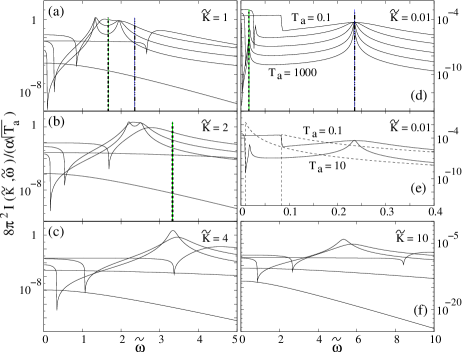
Figure 2: Transresistivity integrand $8\pi^{2}I(\tilde{\omega},\tilde{K})/(\alpha\sqrt{T_{a}})$ vs $\tilde{\omega}$ for different values of $\tilde{K}$ (as labelled). Panels (a), (b), (c), (d) and (f): Five values of $T_{a}$ (separated by a factor 10) have been considered, $T_{a}=0.1\to 1000$, each corresponding to a different solid line (see labelling in panel(d)). Dashed (dashed-double-dot) line corresponds to analytical position of the acoustic (optical) plasmon. Panel(e): Only two values of $T_{a}$ are considered (as labelled); dashed lines correspond to calculations by using the approximation $\chi=\chi_{-}$.

In this Letter we have presented the first, to the best of our knowledge, calculation of Coulomb drag effects between graphene layers, which include temperature-dependent effects. We have also predicted a universal behavior of the Coulomb transresistivity, which is interlayer-distance independent and suggested that this behavior may be experimentally observable. Most of the calculations presented were made for the simplest gapless form of the quasiparticle spectrum in graphene, as expected from tight-binding calculations in the absence of interactions. These results, can be easily generalized to take into account the possible opening of a dielectric gap $\Delta$ in the quasiparticle spectrum Kopelevich:2002 ; Khveshchenko-Gorbar . The interplay of this gap with the temperature and chemical potential may lead to even richer physics and applications.

I Acknowledgments

We thank V.P. Gusynin, V.M. Loktev and J. Dobson for helpful discussions. S.G.Sh. is also grateful to the members of ISI for the friendly support and hospitality.

References

- (1) Y. Kopelevich, P. Esquinazi, J.H.S. Torres, R.R. da Silva, H. Kempa, F. Mrowka, and R. Ocana, Studies of High Temperature Superconductors, Vol. 45, pp. 59-106 (2003); cond-mat/0209442.
- (2) J. Gonzalez, F. Guinea, M.A.H. Vozmediano, Phys. Rev.B 59, 2474 (1999).
- (3) J. Gonzalez, F. Guinea, M.A.H. Vozmediano, Phys. Rev.B 63, 134421 (2001).
- (4) D.V. Khveshchenko, Phys. Rev. Lett. 87, 246802 (2001); E.V. Gorbar, V.P. Gusynin, V.A. Miransky, and I.A. Shovkovy, Phys. Rev. B 66, 045108 (2002).
- (5) M.B. Pogrebinskii, Fiz. Tekh. Poluprovodn. 11, 637 (1997) [Sov. Phys. Semicond. 11, 372 (1977)]; P.J. Price, Physica (Amsterdam) 117B, 750 (1983).
- (6) See e.g. A.G. Rojo, J. Phys.:Condens. Matter 11, R31 (1999), and references therein.
- (7) A. Kamenev and Y. Oreg, Phys. Rev. B 52, 7516 (1995); K. Flensberg, B. Y.-K. Hu, A.-P. Jauho, J.M. Kinaret, Phys. Rev. B 52, 14761 (1995).
- (8) I. D’Amico, G. Vignale, Phys. Rev.B 68, 045307 (2003).
- (9) A. Larkin and A. Varlamov, Theory of fluctuations in superconductors, Clarendon Press, Oxford, 2004.
- (10) I.A. Luk’yanchuk and Y. Kopelevich, cond-mat/0402058.
- (11) A.M. Tsvelik, Quantum Field Theory in Condensed Matter Physics, Cambridge University Press, 1995. Chap. 12.
- (12) R. Pisarski, Phys. Rev. D 29, 2423 (1984); T.W. Appelquist, M. Bowick, D. Karabali, and L.C.R. Wijewardhana, Phys. Rev. D 33, 3704 (1984).
- (13) By inspecting Eq. (1), we then expect that our results for the drag transresistivity will be more reliable for relatively small temperatures () and finite interlayer distance ().
- (14) K. Flensberg and B. Y.-K. Hu, Phys. Rev. Lett. 73, 3572 (1994); Phys. Rev. B 52, 14796 (1995).
- (15) We underline that, depending on the different considered, the same dimensionless temperature may correspond to low or high temperatures – for example for and , corresponds to K and K respectively.
- (16) A.M. Lunde and A.-P.Jauho, Semicond. Sci. Technol. 19, 1 (2004).