Weak ferromagnetism in antiferromagnets: Fe₂O₃ and La₂CuO₄

Abstract

The problem of weak ferromagnetism in antiferromagnets due to canting of magnetic moments was treated using Green’s function technique. At first the eigenvalues and eigenfunctions of the electronic Hamiltonian corresponding to collinear magnetic configuration are calculated which are then used to determine first and second variations of the total energy as a function of the magnetic moments canting angle. Spin-orbit coupling is taken into account via perturbation theory. The results of calculations are used to determine an effective spin Hamiltonian. This Hamiltonian can be mapped on conventional spin Hamiltonian that allows to determine parameters of isotropic and anisotropic (Dzyaloshinskii-Moriya) exchange interactions. The method was applied to the typical antiferromagnets with weak ferromagnetism Fe₂O₃ and La₂CuO₄. The obtained directions and values of the magnetic moments canting angles are in a reasonable agreement with experimental data.

Heisenberg Hamiltonian is a basis of most theoretical investigations of transition metal compounds magnetism. Heisenberg ; Anderson ; dagotto The essential part of these investigation is determination of exchange interaction parameters J_ij. It can be done in a phenomenological way by fitting those parameters to reproduce experimental data (temperature dependence of magnetic susceptibility and magnon dispersion curves obtained in inelastic neutron scattering measurements).VOPO However much more physically appealing is to obtain them in ab-initio calculations. In most cases it was done via calculating total energy values for various different magnetic moments configurations. Mapping on Heisenberg Hamiltonian gave a system of linear equation for J_ij (for example see Ref. Pickett, ). This procedure becomes inconvenient for the systems with a large number of long range competing exchange interactions like in (VO)₂P₂O₇, NaV₂O₅, Cu₂Te₂O₅X₂ (X=Br,Cl), etc. lemmens

In 1987 A.I. Lichtenstein et al. Liechtenstein proposed the calculation method that does not use total energy differences. They determined exchange interaction parameters via calculating second variation of total energy $\delta^{2}E$ for small deviation of magnetic moments from the collinear magnetic configuration. The expression for this second variation was derived analytically and required for its evaluation calculation of the integral over production of one-electron Green functions. This method was since then successfully applied to the various transition metal compounds. solovyev1 ; Korotin99 ; Korotin00 ; Mn12

The combination of low symmetry and spin-orbit coupling was shown by Dzyaloshinskii dzialoshinski and Moriya moriya to give rise to anisotropic exchange coupling. Moriya has shown how the processes involving an additional virtual transition due to spin-orbit coupling can cause an anisotropic exchange interaction as a correction to the isotropic Anderson superexchange term and introduced new term in spin Hamiltonian which is Dzyaloshinskii-Moriya interaction (DM). Solovyev et al. solovyev had shown that Dzyaloshinskii-Moriya interaction parameters can be calculated using perturbation theory and Green’s function technique and described the canting of magnetic moments of LaMnO₃. Recently, Katsnelson and Lichtenstein katsnelson derived the general expression for Dzyaloshinskii-Moriya interaction term in LDA++ approach.

This paper is devoted to the problem of first-principles theoretical description of weak ferromagnetism in antiferromagnets, specifically to the task of calculating weak ferromagnetic moment value and direction of spin canting. For this we consider first and second variations of total energy of the system at small deviation of magnetic moments from collinear configuration with spin-orbit coupling introduced as a perturbation using Green’s function technique. We show that there is an additional on-site term that was not taken into account in previous work, solovyev which gives significant contribution to weak ferromagnetic moment. Basing on the results of the calculations we propose effective single site Hamiltonian. This Hamiltonian is sufficient for solving the problem of spin canting but it also can be rewritten to the conventional form containing isotropic and anisotropic exchange interaction terms. We have applied our method for weak ferromagnetism in Fe₂O₃, the classical system which was used by Moriya in his pioneering work, moriya and in antiferromagnetic cuprate La₂CuO₄ in low temperature orthorhombic phase, estimated ferromagnetic moments values on the metallic ions in these compounds and determined the plane of spin canting.

Briefly, this paper is organized as follows. In Sec.I we describe the method for calculation spin Hamiltonian parameters responsible for magnetic moments canting. Sec.II contains the results of our calculations for Fe₂O₃ and La₂CuO₄ crystals. In Sec.III we discuss and briefly summarize our results.

I Method

According to the Andersen’s “local force theorem” machintosh ; methfessel ; heine the total energy variation $\delta E$ under the small perturbation from the ground state coincides with the sum of one-particle energy changes for the occupied states at the fixed ground state potential. In the first order for the perturbations of the charge and spin densities one can find the following relation Liechtenstein :

$$\delta E=\int_{-\infty}^{E_{F}}\mathrm{d}\epsilon\,\epsilon\,\delta n(\epsilon)=\epsilon_{F}\,\delta z-\int_{-\infty}^{E_{F}}\mathrm{d}\epsilon\,\delta N(\epsilon)$$

$$=-\int_{-\infty}^{E_{F}}\,\mathrm{d}\epsilon\,\delta N(\epsilon),$$ (1)

here $n(\epsilon)=\mathrm{d}N/\mathrm{d}\epsilon$ is the density of electron state, N($\epsilon$) is integrated density of electron state and $\epsilon_{F}$ is Fermi energy. In the case of magnetic excitation the change of total number of electrons $\delta z$ equals zero. The Green function G is formally expressed in the usual way $G=(\epsilon-H)^{-1}$. One can express density of states and integrated density of states via Green function G:

$$n(\epsilon)=-\frac{1}{\pi}\,Im\,Sp\,G(\epsilon)$$ (2)

and

$$N(\epsilon)=-\frac{1}{\pi}\,Im\,Sp\,\ln(\epsilon-H).$$ (3)

Then the variation of integrated density of state is given by

$$\delta N(\epsilon)=\frac{1}{\pi}\,Im\,Sp\,[\delta H\,G].$$ (4)

Therefore the first and second variations of total energy of the system take the following forms:

$$\delta E=-\frac{1}{\pi}\,\int_{-\infty}^{E_{F}}\mathrm{d}\epsilon\,Im\,Sp\,(\delta H\,G)$$ (5)

and

$$\delta^{2}E=-\frac{1}{\pi}\,\int_{-\infty}^{E_{F}}\mathrm{d}\epsilon\,Im\,Sp\,(\delta^{2}H\,G\,+\,\delta H\,G\,\delta H\,G).$$ (6)

Operator of spin rotation on the site $j$ on the angle $|\vec{\delta}\phi|$ around direction $\vec{n}\,=\,\frac{\vec{\delta\phi}}{|\vec{\delta\phi}|}$ is given by

$$\widehat{U}=e^{\frac{1}{2}\,i\,\vec{\delta\phi}\,\widehat{\vec{\sigma}}}$$ (7)

where $\widehat{\vec{\sigma}}\,=\,(\widehat{\sigma}_{x},\widehat{\sigma}_{y},\widehat{\sigma}_{z})$ are Pauli matrices. For small $|\vec{\delta\phi}|$ values we can expand the spin rotation operator in following way

$$\widehat{U}\,=\,1\,+\,\frac{1}{2}\,i\,\vec{\delta\phi}\,\widehat{\vec{\sigma}}-\frac{1}{8}\,(\vec{\delta\phi}\,\widehat{\vec{\sigma}})^{2}.$$ (8)

New Hamiltonian of the system after rotation of the spin on j site around direction $\vec{n}$ on the angle $|\vec{\delta\phi}|$

$$\widehat{\widetilde{H}}=\widehat{U^{{\dagger}}}\widehat{H}\widehat{U}$$ (9)

The first variation over the angle of rotation is expressed in following form:

$$\delta\widehat{H}=\frac{1}{2}\,i\,\vec{\delta\phi}\,[\widehat{H},\widehat{\vec{\sigma}}]$$ (10)

In the basis $|ilm\sigma\rangle$ (where $i$ is site, $l$ is orbital quantum number, $m$ is magnetic quantum number and $\sigma$ is spin index) the Hamiltonian matrix takes the form $H_{ilm,jlm^{\prime}}^{\sigma\sigma^{\prime}}=\langle ilm\sigma|\widehat{H}|jlm^{\prime}\sigma^{\prime}\rangle$. For simplicity below we drop the index of orbital and magnetic quantum numbers and leave spin and site indexes. We assume that without spin-orbit interaction the ground state corresponds to the collinear magnetic configuration at which all spin moments lie along z axis. Therefore the Hamiltonian matrix H${}_{ij}^{\sigma\sigma^{\prime}}$ is diagonal in the spin subspace

$$H_{ij}=\left(\begin{array}[]{cc}{\bf H_{ij}^{\uparrow}}&0\\ 0&{\bf H_{ij}^{\downarrow}}\end{array}\right).$$

One can rewrite the first variation of Hamiltonian Eq.(10) in the following form

$$\delta H_{jj}\,=\,i\,\delta\phi^{x}_{j}\left(\begin{array}[]{cc}0&\frac{\Delta_{j}}{2}\\ -\frac{\Delta_{j}}{2}&0\end{array}\right)\,+\,\delta\phi^{y}_{j}\left(\begin{array}[]{cc}0&\frac{\Delta_{j}}{2}\\ \frac{\Delta_{j}}{2}&0\end{array}\right),$$ (15)

where $\Delta_{j}\,=\,{\bf H^{\uparrow}_{jj}}\,-\,{\bf H^{\downarrow}_{jj}}$. It is easy to show that the second variation of Hamiltonian is given by

$$\delta^{2}H_{jj}=\delta^{2}\phi^{x}_{j}\left(\begin{array}[]{cc}-\frac{\Delta_{j}}{2}&0\\ 0&\frac{\Delta_{j}}{2}\end{array}\right)+\delta^{2}\phi^{y}_{j}\left(\begin{array}[]{cc}-\frac{\Delta_{j}}{2}&0\\ 0&\frac{\Delta_{j}}{2}\end{array}\right).$$ (20)

The rotation of spin moment around z axis doesn’t change the energy of the system therefore the term with $\delta\phi^{z}$ is absent in Eq.(15,20).

Then we take into account the spin-orbit coupling via perturbation theory. The Green function in the first order perturbation theory with respect to the spin-orbit coupling can be written as

$$\tilde{G}_{ij}\,=\,G_{ij}\,+\,\sum_{k}G_{ik}\,H^{so}_{k}\,G_{kj},$$ (21)

here $H^{so}_{k}=\lambda_{k}\,\vec{L}\,\vec{S}$, i, j and k denote site, G^ij is Green function of system with collinear magnetic configuration, and $\lambda_{k}$ is spin-orbit coupling constant. The first variation of total energy Eq.(5) takes the form:

$$\delta E\,=\,-\frac{1}{\pi}\,\sum_{i}\int_{-\infty}^{E_{F}}\mathrm{d}\epsilon\,Im\,Sp$$

$$\times(\delta H_{i}\,G_{ii}\,+\,\sum_{k}\,\delta H_{i}\,G_{ik}\,H^{so}_{k}\,G_{ki}).$$ (22)

The first term in Eq.(22) is zero. The second term can be expressed as a following sum

$$\delta E\,=\,\sum_{i}A^{x}_{i}\,\delta\phi^{x}_{i}\,+\,A^{y}_{i}\,\delta\phi^{y}_{i},$$ (23)

where

$$A^{x}_{i}=\sum_{k}B^{x}_{ik}=\,-\frac{1}{2\pi}\int_{-\infty}^{E_{F}}\,\mathrm{d}\epsilon\,Re$$

$$\times\sum_{k}\,(\Delta_{i}\,G_{ik}^{\downarrow}\,H^{so}_{k\,\downarrow\uparrow}\,G_{ki}^{\uparrow}-\,\Delta_{i}\,G_{ik}^{\uparrow}\,H^{so}_{k\,\uparrow\downarrow}\,G_{ki}^{\downarrow})$$ (24)

and

$$A^{y}_{i}=\sum_{k}B^{y}_{ik}=\,-\frac{1}{2\pi}\int_{-\infty}^{E_{F}}\,\mathrm{d}\epsilon\,Im$$

$$\times\sum_{k}\,(\Delta_{i}\,G_{ik}^{\downarrow}\,H^{so}_{k\,\downarrow\uparrow}\,G_{ki}^{\uparrow}\,+\,\Delta_{i}\,G_{ik}^{\uparrow}\,H^{so}_{k\,\uparrow\downarrow}\,G_{ki}^{\downarrow}).$$ (25)

We consider the situation when all spins lie along z axis and therefore the rotation around it does not change the energy of system. In order to find A${}^{z}_{i}$ component of the magnetic torque vector $\vec{A}_{i}$ we change the coordinate system in the following way (x,y,z)$\rightarrow$(z,y,-x) (rotation around y axis):

$$\tilde{H}^{so}\,=\,\frac{1}{2}\left(\begin{array}[]{cc}1&1\\ -1&1\end{array}\right)\,\left(\begin{array}[]{cc}H^{so}_{\uparrow\uparrow}&H^{so}_{\uparrow\downarrow}\\ H^{so}_{\downarrow\uparrow}&H^{so}_{\downarrow\downarrow}\end{array}\right)\,\left(\begin{array}[]{cc}1&-1\\ 1&1\end{array}\right).$$ (32)

Therefore A${}^{x}_{i}$ component in new coordinate system is A${}^{z}_{i}$ in the old one:

$$A^{z}_{i}=\sum_{ik}B^{z}_{ik}=\,-\frac{1}{4\pi}\int_{-\infty}^{E_{F}}\,\mathrm{d}\epsilon\,Re$$

$$\times\sum_{k}\,(\Delta_{i}\,G_{ik}^{\uparrow}\,(H^{so}_{k\,\uparrow\uparrow}\,-\,H^{so}_{k\,\downarrow\downarrow})\,G_{ki}^{\downarrow}$$

$$-\Delta_{i}\,G_{ik}^{\downarrow}\,(H^{so}_{k\,\uparrow\uparrow}\,-\,H^{so}_{k\,\downarrow\downarrow})\,G_{ki}^{\uparrow}).$$ (33)

In contrast to the first variation $\delta E$, the second variation of total energy $\delta^{2}E$ for small deviations of magnetic moments from ground-state collinear magnetic configuration has nonzero value without taking into account spin-orbit coupling:

$$\delta^{2}E\,=\,-\frac{1}{\pi}\,\int_{-\infty}^{E_{F}}\mathrm{d}\epsilon\,Im\,Sp\,(\frac{1}{2}\,\sum_{i}\delta^{2}H_{ii}G_{ii}$$

$$+\,\frac{1}{2}\,\sum_{j}\,\delta^{2}H_{jj}G_{jj}\,+\,\sum_{ij}\,\delta H_{i}\,G_{ij}\,\delta H_{j}\,G_{ji}),$$ (34)

where

$$Sp\,(\delta^{2}H_{ii}\,G_{ii})\,=\,\frac{1}{2}\delta^{2}\phi^{x}_{i}\Delta_{i}(G_{ii}^{\downarrow}\,-\,G_{ii}^{\uparrow})$$

$$+\,\frac{1}{2}\delta^{2}\phi^{y}_{i}\Delta_{i}(G_{ii}^{\downarrow}\,-\,G_{ii}^{\uparrow})$$ (35)

and

$$Sp\,(\delta H_{i}\,G_{ij}\,\delta H_{j}\,G_{ji})\,=\,\frac{1}{2}\,\delta\phi^{x}_{i}\,\delta\phi^{x}_{j}\,(\Delta_{i}\,G^{\downarrow}_{ij}\,\Delta_{j}\,G^{\uparrow}_{ji})$$

$$+\,\frac{1}{2}\,\delta\phi^{y}_{i}\,\delta\phi^{y}_{j}\,(\Delta_{i}\,G^{\downarrow}_{ij}\,\Delta_{j}\,G^{\uparrow}_{ji}).$$ (36)

Using the condition $G_{ii}^{\uparrow}\,-\,G_{ii}^{\downarrow}\,=\,(G^{\uparrow}\Delta\,G^{\downarrow})_{ii}\,=\,\sum_{j}G_{ij}^{\uparrow}\Delta_{j}\,G_{ji}^{\downarrow}$ one may rewrite Eq.(34) in following form:

$$\delta^{2}E\,=\,\frac{1}{4\pi}\,\int_{-\infty}^{E_{F}}\mathrm{d}\epsilon\,Im\,\sum_{ij}(\Delta_{i}\,G_{ij}^{\downarrow}\,\Delta_{j}\,G_{ji}^{\uparrow})$$

$$\times((\delta\phi_{i}^{x}\,-\delta\phi_{j}^{x})^{2}\,+\,(\delta\phi_{i}^{y}\,-\delta\phi_{j}^{y})^{2}).$$ (37)

One can see that the Eq.(37) contains only $x$ and $y$ components of $\vec{\delta\phi}$. In order to include $z$ component one can use the same rotation of coordinate system as for the site magnetic torque vector $\vec{A}$ Eq.(32). Finally, we obtain the following function of the total energy over angle $\vec{\delta\phi}$:

$$\Delta E\,=\,\sum_{i}\vec{A}_{i}\,\vec{\delta\phi_{i}}\,+\,\frac{1}{2}\,\sum_{ij}\,J_{ij}\,|\vec{\delta\phi_{i}}\,-\,\vec{\delta\phi_{j}}|^{2},$$ (38)

where

$$J_{ij}\,=\,\frac{1}{4\pi}\,\int_{-\infty}^{E_{F}}\mathrm{d}\epsilon\,Im(\Delta_{i}\,G_{ij}^{\downarrow}\,\Delta_{j}\,G_{ji}^{\uparrow}).$$ (39)

The aim of this paper is description of canted magnetism in transition metal compounds caused by spin-orbit coupling. For this we have used the expression Eq.(38) for the total energy as a function of canting angle. In order to solve the problem of the weak ferromagnetism in antiferromagnets we suppose that the crystal is an antiferromagnet containing two sublattices $1$ and $2$, with the same canting angle for the atoms belonging to the same sublattice. With this assumption the Eq.(38) is reduced to the following form:

$$\Delta E\,=\,\vec{A}_{1}\,\vec{\delta\phi_{1}}\,+\,\vec{A}_{2}\,\vec{\delta\phi_{2}}\,+\,\sum_{j>1}J_{1j}\,|\vec{\delta\phi_{1}}\,-\,\vec{\delta\phi_{2}}|^{2}.$$ (40)

Our results for Fe₂O₃ and La₂CuO₄ demonstrated that $\vec{A}_{1}$ = - $\vec{A}_{2}$ (torque vector has an opposite sign for the atoms belonging to the different sublattices). That gives:

$$\Delta E\,=\,\vec{A}_{1}\,(\vec{\delta\phi_{1}}-\vec{\delta\phi_{2}})\,+\,\sum_{j>1}J_{1j}\,|\vec{\delta\phi_{1}}-\vec{\delta\phi_{2}}|^{2}.$$ (41)

If we further suppose that the deviations of magnetic moments from the average direction defined by $\vec{\delta\phi_{i}}$ have the same absolute value but different sign for both sublattices, then Eq.(41) takes the following form (we suppose that magnetic moments lie in plane perpendicular to site magnetic torque vector $\vec{A}$ and canting occurs in the same plane)

$$\Delta E\,=\,2\,\vec{A}_{1}\,\vec{\delta\phi_{1}}\,+\,4\,\sum_{j>1}J_{1j}\,|\vec{\delta\phi_{1}}|^{2}.$$ (42)

Then we find the value of $|\vec{\delta\phi_{1}}|$ where $\Delta E$ has a minimum:

$$|\vec{\delta\phi_{1}}|\,=\,\frac{|\vec{A}_{1}|}{4\,\sum_{j>1}J_{1j}}.$$ (43)

The next step is to establish a connection between Eq.(38) and conventional spin Hamiltonian

$$H\,=\,H_{DM}+H_{exch}\,=\,\sum_{i\not=j}\vec{D}_{ij}\,[\vec{e}_{i}\times\vec{e}_{j}]$$

$$+\,\sum_{i\not=j}\,J_{ij}\,\vec{e}_{i}\vec{e}_{j},$$ (44)

where e_i is unit vector in the direction of the $i$th site magnetization, J_ij is exchange interaction and $\vec{D}_{ij}$ is Dzyaloshinskii-Moriya vector. One can rewrite the second term in Eq.(44) as $H_{exch}\,=\,\sum_{ij}J_{ij}|\vec{e}_{i}|\,|\vec{e}_{j}|cos(\theta_{ij})$. In the limit of small canting angle values we can assume that $cos(\theta_{ij})\,=\,1-|\vec{\delta\phi_{i}}-\vec{\delta\phi_{j}}|^{2}/2$ and exchange interaction energy for antiferromagnetic configuration has a form:

$$\Delta H_{exch}\,=\,\frac{1}{2}\sum_{ij}J_{ij}\,|\vec{\delta\phi_{i}}-\vec{\delta\phi_{j}}|^{2}.$$ (45)

Therefore in the limit of small $\vec{\delta\phi}$ we can directly map the second term of total energy variation Eq.(38) onto first term in spin Hamiltonian Eq.(44).

The first term in Eq.(38) describes the deviation of the spin moment on the site $i$ from the initial collinear spin configuration direction. We assume that this initial spin direction on the site $i$ is defined by the direction of Weiss mean-field $\vec{H}^{WF}_{i}\,=\,\sum_{j(\not=i)}J_{ij}\,\vec{e}_{j}$ (corresponding unit vector is $\vec{e}^{\,\,0}_{i}=\frac{\vec{H}^{WF}_{i}}{|\vec{H}^{WF}_{i}|}$). Therefore we can map the first term in Eq.(38) on the spin Hamiltonian

$$H_{dev}\,=\,\sum_{i}\vec{A}_{i}\,[\vec{e}^{\,\,0}_{i}\times\vec{e}_{i}]$$ (46)

describing the deviation of spin moments away from the direction $\vec{e}^{\,\,0}_{i}$ of external Weiss field. (We have used here the connection between rotation vector $\vec{\delta\phi_{i}}$ and the change of the magnetic moment unit vector $\delta\vec{e}_{i}=\vec{e}_{i}-\vec{e}^{\,\,0}_{i}$: $\delta\vec{e}_{i}=[\vec{\delta\phi_{i}}\times\vec{e}^{\,\,0}_{i}]$.) In order to demonstrate the connection between $\vec{A}_{i}$ and $\vec{D}_{ij}$ one can rewrite the Eq.(46) in the following form:

$$H_{dev}\,=\,\frac{1}{2}(\sum_{i}\vec{A}_{i}\,[\frac{\vec{H}^{WF}_{i}}{|\vec{H}^{WF}_{i}|}\times\vec{e}_{i}]$$

$$+\,\sum_{j}\vec{A}_{j}\,[\frac{\vec{H}^{WF}_{j}}{|\vec{H}^{WF}_{j}|}\times\vec{e}_{j}]).$$ (47)

Using our definition of $\vec{H}^{WF}_{i}$ we obtain:

$$H_{dev}\,=\,\frac{1}{2}(\sum_{ij}\frac{\vec{A}_{i}}{|\vec{H}^{WF}_{i}|}J_{ij}[\vec{e}_{j}\times\vec{e}_{i}]$$

$$+\,\sum_{ij}\frac{\vec{A}_{j}}{|\vec{H}^{WF}_{j}|}J_{ij}[\vec{e}_{i}\times\vec{e}_{j}]).$$ (48)

This gives us the following expression for parameter $\vec{D}_{ij}$ of spin Hamiltonian Eq.(44):

$$\vec{D}_{ij}\,=\,\frac{1}{2}\,J_{ij}\,(\frac{\vec{A}_{j}}{|\vec{H}^{WF}_{j}|}\,-\,\frac{\vec{A}_{i}}{|\vec{H}^{WF}_{i}|}).$$ (49)

Therefore the components of Dzyaloshinskii-Moriya interaction vector are given by

$$D^{x}_{ij}\,=\,-\frac{1}{4\pi}\,J_{ij}\,\int_{-\infty}^{E_{F}}\mathrm{d}\epsilon\,Re\,\sum_{k}$$

$$\times(\frac{\Delta_{j}\,G_{jk}^{\downarrow}\,H^{so}_{k\,\downarrow\uparrow}\,G_{kj}^{\uparrow}\,-\,\Delta_{j}G_{jk}^{\uparrow}\,H^{so}_{k\,\uparrow\downarrow}\,G_{kj}^{\downarrow}}{|\vec{H}^{WF}_{j}|}$$

$$-\,\frac{\Delta_{i}\,G_{ik}^{\downarrow}\,H^{so}_{k\,\downarrow\uparrow}\,G_{ki}^{\uparrow}\,-\,\Delta_{i}G_{ik}^{\uparrow}\,H^{so}_{k\,\uparrow\downarrow}\,G_{ki}^{\downarrow}}{|\vec{H}^{WF}_{i}|}),$$ (50)

$$D^{y}_{ij}\,=\,-\frac{1}{4\pi}\,J_{ij}\,\int_{-\infty}^{E_{F}}\mathrm{d}\epsilon\,Im\,\sum_{k}$$

$$\times(\frac{\Delta_{j}\,G_{jk}^{\downarrow}\,H^{so}_{k\,\downarrow\uparrow}\,G_{kj}^{\uparrow}\,+\,\Delta_{j}G_{jk}^{\uparrow}\,H^{so}_{k\,\uparrow\downarrow}\,G_{kj}^{\downarrow}}{|\vec{H}^{WF}_{j}|}$$

$$-\,\frac{\Delta_{i}\,G_{ik}^{\downarrow}\,H^{so}_{k\,\downarrow\uparrow}\,G_{ki}^{\uparrow}\,+\,\Delta_{i}G_{ik}^{\uparrow}\,H^{so}_{k\,\uparrow\downarrow}\,G_{ki}^{\downarrow}}{|\vec{H}^{WF}_{i}|}),$$ (51)

$$D^{z}_{ij}\,=-\,\frac{1}{8\pi}\,J_{ij}\,\int_{-\infty}^{E_{F}}\mathrm{d}\epsilon\,Re\,\sum_{k}$$

$$\times(\frac{\Delta_{j}\,G_{jk}^{\uparrow}\,(H^{so}_{k\,\uparrow\uparrow}\,-\,H^{so}_{k\,\downarrow\downarrow})\,G_{kj}^{\downarrow}}{|\vec{H}^{WF}_{j}|}$$

$$-\frac{\Delta_{j}\,G_{jk}^{\downarrow}\,(H^{so}_{k\,\uparrow\uparrow}\,-\,H^{so}_{k\,\downarrow\downarrow})\,G_{kj}^{\uparrow}}{|\vec{H}^{WF}_{j}|}$$

$$-\frac{\,\Delta_{i}\,G_{ik}^{\uparrow}\,(H^{so}_{k\,\uparrow\uparrow}\,-\,H^{so}_{k\,\downarrow\downarrow})\,G_{ki}^{\downarrow}}{|\vec{H}^{WF}_{i}|}$$

$$+\frac{\Delta_{i}\,G_{ik}^{\downarrow}\,(H^{so}_{k\,\uparrow\uparrow}\,-\,H^{so}_{k\,\downarrow\downarrow})\,G_{ki}^{\uparrow}}{|\vec{H}^{WF}_{i}|}).$$ (52)

We have obtained more general expression for Dzyaloshinskii-Moriya interaction parameter in comparison with those presented in paper. solovyev There are two kind of contributions into magnetic torque vector $\vec{A}_{i}$: on-site interaction $\vec{B}_{ii}$ (absent in work solovyev ) and intersite interaction $\vec{B}_{ik}$(i $\not=$ k). We have found that on-site contribution in magnetic torque $\vec{A}$ which was not considered before plays an important role in weak ferromagnetism description.

We have applied the calculation scheme developed above to the typical antiferromagnets with weak ferromagnetism Fe₂O₃ and La₂CuO₄ in low-temperature orthorhombic phase. In order to calculate Green functions corresponding to the collinear spin configurations we used LDA+U approach Anisimov realized in LMTO method within Atomic Sphere Approximation. Andersen

II results

II.1 Fe₂O₃

Weak ferromagnetism or weak non-collinearity of essentially antiparallel magnetic moments was first observed in $\alpha$-hematite, $\alpha$-Fe₂O₃.smith The trigonal crystal of Fe₂O₃ has R${\bar{3}}$c space group. Depending on temperature $\alpha$-hematite may occur in two different antiferromagnetic states: at T $<$ 250 K the spins are along the trigonal axis, and at 250 K $<$ T $<$ 950 K they lie in one of the vertical planes of symmetry making a small angle $1.1\times 10^{-3}$ with basal plane.Flanders ; Bodker In the latter case the $\alpha$-Fe₂O₃ has a net ferromagnetic moment. Dzyaloshinskii has shown that the spin superstructure gives rise to a nonvanishing antisymmetric spin coupling vector which is parallel to the trigonal axis. Moriya moriya gave phenomenological Dzyaloshinski’s explanation a microscopic footing by means of Anderson’s perturbation approach to magnetic superexchange.

Sandratskii $et$ $al$. sandratskii have performed the calculation based on the local approximation to spin-density functional theory (LSDA) using the fully relativistic version of ASW method. In spite of the well-known problem that the LSDA has with a proper determination of the energy gap in semiconducting and insulating materials, the authors sandratskii succeeded in describing a weak ferromagnetism and obtained the ferromagnetic moment of about 0.002 $\mu_{B}$. In the present study we treat the problem of description of weak ferromagnetism in Fe₂O₃ using perturbation theory.

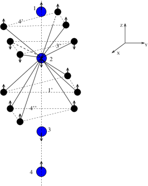
Figure 1: Crystal structure of $\alpha$-Fe₂O₃. Large circles are Fe atoms which belong the smallest unit cell used in the LDA+U calculations. The small circles are Fe atoms which surround Atom 2. Arrows denote the magnetic configuration used in our calculation.

Electronic structure of $\alpha$-hematite calculated using the standard LDA+U approximation Anisimov with on-site Coulomb interaction parameters U = 5 eV, J = 0.88 eV and structure data from newnham is in a good agreement with previous theoretical calculations.Amrit We have obtained the magnetic moment of 4.1 $\mu_{B}$ per Fe atom. This value is a little smaller than those obtained in experiments (4.6-4.9 $\mu_{B}$). The energy gap value of 1.67 eV is also slightly underestimated comparing with experimental data (2.14 eV in paper benjelloun ).

The Brillouin zone integration has been performed in the grid generated by using (6;6;6) divisions. The energy integration has been performed in the complex plane by using 800 energy points on the rectangular contour. The calculated isotropic exchange interactions and contributions in site magnetic torque $\vec{A}_{2}$ are presented in Table I. The simplified crystal structure and the interaction paths are shown in Fig.1.

One can see that the obtained interaction picture is more complicated that those Moriya examined in order to describe the weak ferromagnetism in $\alpha$-hematite.moriya There are strong isotropic exchange interaction with third and fourth neighbours. This agrees well with experimental results samuelsen and theoretical predictions.goodenough The summary exchange of atom 2 with nearest neighbours is given by $J_{2}=\sum_{i\not=2}J_{2\,i}\,=\,$ 189.26 meV.

Table 1: Isotropic exchange interaction parameter and different contributions in components of site magnetic torque of Fe₂O₃ (in meV). The couplings with negative sign are ferromagnetic. d_ij is distance between i and j atoms in a.u. $\vec{R}_{ij}$ is radius vector from i site to j site in units of the lattice constant (5.49 a.u.).

(i, j)	dij	$\vec{R}_{ij}$	Jij	B${}^{x}_{ij}$	B${}^{y}_{ij}$	B${}^{z}_{ij}$
(2,2)	0	(0;0;0)	0	0	0	0.162
(2,1)	5.45	(0;0;-0.99)	8.576	0	0	0.005
(2,3’)	5.60	(-0.5;-0.86;0.20)	-7.3	-0.036	0.015	0.001
(2,3’)	5.60	(1;0;0.20)	-7.3	0.032	0.023	0.001
(2,3’)	5.60	(-0.5;0.86;0.20)	-7.3	0.004	-0.038	0.001
(2,1’)	6.36	(0.5;-0.86;-0.58)	25.224	0.071	0.019	-0.14
(2,1’)	6.36	(-1;0;-0.58)	25.224	-0.052	0.052	-0.14
(2,1’)	6.36	(0.5; 0.86;-0.58)	25.224	-0.019	-0.071	-0.14
(2,4’)	6.99	(0.5;-0.86;0.79)	17.502	0.168	0.063	0.101
(2,4’)	6.99	(-1;0;0.79)	17.502	-0.139	0.114	0.101
(2,4’)	6.99	(0.5;0.86;0.79)	17.502	-0.029	-0.178	0.101
(2,4”)	6.99	(-0.5;-0.86;-0.79)	17.502	0.128	0.094	0.076
(2,4”)	6.99	(1;0;-0.79)	17.502	0.017	-0.158	0.076
(2,4”)	6.99	(-0.5;0.86;-0.79)	17.502	-0.145	0.064	0.076

The components of site magnetic torque vector on the atom 2 are given by $A^{x}_{2}=\sum_{i}B^{x}_{2i}\,=\,$ 0 eV, $A^{y}_{2}=\sum_{i}B^{y}_{2i}\,=\,$ 0 eV and $A^{z}_{2}=\sum_{i}B^{z}_{2i}\,=\,$ 0.281 meV. One can see that the on-site interaction $B^{z}_{22}$ gives the main contribution in $\vec{A}_{2}$. We have calculated also the site magnetic torque of $\vec{A}_{1}$ which has the following components (0;0;-0.281), the same value but the opposite sign comparing with $\vec{A}_{2}$. The value of canting angle of $|\vec{\delta\phi}|\,=\,0.4\times 10^{-3}$ calculated with Eq.(43) is of the correct order of magnitude but is more than two time smaller than experimental data $1.1\times 10^{-3}$ (Ref. Flanders, ; Bodker, ). The reason for the difference between experimentally observed and calculated here values of canting angle could be the necessity to take into consideration the higher order terms with respect to spin-orbit coupling which were not considered in the present study.

It is easy to show that in the case when all spin lie along z axis there is no canting of the spin moments. On the other hand if direction of Weiss field is perpendicular to z axis the canting exists and the system has weak ferromagnetic moment. This picture fully agrees with experimental and theoretical data. moriya ; Flanders ; Bodker

II.2 La₂CuO₄

In the case of the cuprates Dzyaloshinskii-Moriya interaction is the leading source of anisotropy, since single-ion anisotropy does not occur due to the S=$\frac{1}{2}$ nature of the spins on the Cu²⁺ sites. The experimental data Thio ; Kastner demonstrate that in case of low temperature orthorhombic phase the spins do not lie exactly in the Cu-O planes, but are canted out of the plane by a small angle (0.17^∘). Coffey and coworkers Coffey made complete examination of the anisotropic exchange interaction in orthorhombic phase based on a symmetry consideration. They assumed rotation axis of the the CuO₆ as a direction of antisymmetric exchange interaction and obtained that the spins are canted in plane which is perpendicular Dzyaloshinskii-Moriya vector.

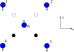
Figure 2: The schematic crystal structure of La₂CuO₄ in low temperature orthorhombic phase. The open circles are oxygen atoms which are tilted up out of the Cu plane, the black circles are oxygen atoms tilted down out the Cu plane. The big gray circles are copper atoms. Arrows denote the magnetic configuration used in LDA+U calculations with spin moments lie along z axis.

The first attempt at a microscopic calculation of the Dzyaloshinskii-Moriya anisotropy for La₂CuO₄ in low temperature orthorhombic and tetragonal phases was made by Coffey, Rice, and Zhang.Rice They have neglected the symmetric anisotropic exchange interaction which is of the second order with respect to the spin-orbit coupling and can be written in spin Hamiltonian in the following form:

$$H_{ij}\,=\,\vec{S_{i}}\,M_{ij}\,\vec{S_{j}},$$

where M_ij is a symmetric $3\,\times\,3$ tensor.

Shekhtman, Entin-Wolhman, and Aharony shekhtman have shown that symmetric anisotropic exchange interaction can not be neglected, since its contribution to the magnetic energy is of the same order of magnitude as that of the antisymmetric anisotropic exchange interaction (Dzyaloshinskii-Moriya). On the basis of our results (as we show below) we can conclude also that taking into account the second order terms with respect to the spin-orbit coupling must be important.

We have performed the LDA+U calculations for La₂CuO₄ in low temperature orthorhombic phase using structural data for Nd doped La₂CuO₄,Axe with on-site Coulomb interaction parameters U = 10 eV, J =1 eV (the same as used in work Korotin ). The schematic structure of Cu-O layer of La₂CuO₄ in low temperature orthorhombic phase is presented in Fig.2.

The experimental value of the energy gap is reported to be about 2 eV (Ref. cooper, ). Our gap value of 1.94 eV is in a good agreement with experimental data. The calculated magnetic moment value on Cu atom is 0.61 $\mu_{B}$ which also agrees well with experiment.Yamada

Table 2: Isotropic exchange J_0j and the components of different contributions in site magnetic torque $\vec{A}_{0}$ (in meV). $\vec{R}_{ij}$ is radius vector from i site to j site in units of the lattice constant (10.14 a.u.).

(i, j)	$\vec{R}_{ij}$	Jij	B${}^{x}_{ij}$	B${}^{y}_{ij}$	B${}^{z}_{ij}$
(0,0)	(0;0;0)	0	0.101	0	0
(0,1)	(-0.5;0.5;0)	14.576	0.020	-0.032	-0.005
(0,2)	(0.5;0.5;0)	14.576	0.020	0.032	0.005
(0,3)	(0.5;-0.5;0)	14.576	0.020	-0.032	-0.005
(0,4)	(-0.5;-0.5;0)	14.576	0.020	0.032	0.005

We have performed calculations of isotropic exchange interactions and the different contributions to site magnetic torque components (Table II) using the energy integration in the complex plane with 700 energy points on the rectangular contour and the Brillouin zone integration has been performed in the grid generated by using (6;6;6) divisions. The obtained values of exchange interaction parameters are in a good agreement with results of previous calculations for low temperature tetragonal phase Korotin and experimental estimations.Thio The exchange interactions with next neighbours are negligibly small. The summary exchange and the components of site magnetic torque are given by $J_{0}\,=\sum_{i\not=0}J_{0\,i}\,=\,$ 58.304 meV, $A^{x}_{0}\,=\,$ 0.18 meV, $A^{y}_{0}\,=\,$ 0 meV and $A^{z}_{0}\,=\,$ 0 eV. We obtained that $\vec{A}_{2}$=(-0.18;0;0), again of the same value but the opposite sign comparing with $\vec{A}_{0}$. It means that the system has net ferromagnetic moment if spins lie in plane which is perpendicular to $x$ axis, which is axis of rotation of oxygen octahedra. This fully agrees with results of previous theoretical works.Thio ; Coffey ; Rice The obtained value of canting angle $|\vec{\delta\phi}|\,=\,0.77\times 10^{-3}$ is about three times smaller than those experimentally observed $2.2\div 2.9\times 10^{-3}$ (Ref. Thio, ; Kastner, ).

Again as for Fe₂O₃ we expect that the inclusion of second order spin-orbit coupling terms could improve the agreement. Such calculations are in progress.

III Conclusion

We present a method for calculation of spin Hamiltonian parameters responsible for magnetic moments canting. The effective Hamiltonian for canted magnetism was proposed. We shown that the parameters of this model Hamiltonian can be obtained from first-principles calculations. Using the developed method we described the weak ferromagnetism in Fe₂O₃ and La₂CuO₄. It was shown that on-site contribution $\vec{B}_{ii}$ in site magnetic torque $\vec{A}_{i}$ plays the crucial role for net ferromagnetic moment of Fe₂O₃ and La₂CuO₄ in low temperature orthorhombic phase.

IV ACKNOWLEDGMENTS

We would like to thank A.I. Lichtenstein who initiated this investigation. We also wishes to thank F. Mila, M. Troyer, T.M. Rice, M. Sigrist, M. Elhajal and M.A. Korotin for helpful discussions. This work is supported by the scientific program ”Russian Universities” yp.01.01.059 and Russian Foundation for Basic Research grant RFFI 04-02-16096.

References

- (1) W. Heisenberg, Z. Physik 49, 619 (1928).
- (2) P.W. Anderson, Phys. Rev. 115, 2 (1959); Solid State Physics 14, 99 (Academic, New York 1963).
- (3) E. Dagotto and T.M. Rice, Science 271, 618 (1996).
- (4) A.W. Garrett, S.E. Nagler, D.A. Tennant, B.C. Sales, and T. Barnes, Phys. Rev. Lett. 79, 745 (1997).
- (5) W.E. Pickett, Phys. Rev. Lett. 79, 1746 (1997).
- (6) P. Lemmens, G. Güntherodt, and C. Gros, Physics Reports 375, 1 (2003).
- (7) A.I. Lichtenstein, M.I. Katsnelson, V.P. Antropov, and V.A. Gubanov, J. Magn. Magn. Mater. 67, 65 (1987).
- (8) I.V. Solovyev and K. Terakura, Phys. Rev. B 58, 15496 (1998).
- (9) M.A. Korotin, I.S. Elfimov, V.I. Anisimov, M. Troyer, and D.I. Khomskii, Phys. Rev. Lett. 83, 1387 (1999).
- (10) M.A. Korotin, V.I. Anisimov, T. Saha-Dasgupta, and I. Dasgupta, J. Phys.: Condens. Matter 12, 113 (2000).
- (11) D.W. Boukhvalov, A.I. Lichtenstein, V.V. Dobrovitski, M.I. Katsnelson, B.N. Harmon, V.V. Mazurenko, and V.I. Anisimov, Phys. Rev. B 65, 184435 (2002).
- (12) I. Dzyaloshinskii, J. Phys. Chem. Solids 4, 241 (1958).
- (13) Toru Moriya, Phys. Rev. 120, 91 (1960).
- (14) I.V. Solovyev, N. Hamada and K. Terakura, Phys. Rev. Lett. 76, 4825 (1996).
- (15) M.I. Katsnelson and A.I. Lichtenstein, Phys. Rev. B 61, 8906 (2000).
- (16) A.R. Machintosh and O.K. Andersen, in: Electrons at the Fermin Surface, ed. M. Springford (Cambridge Univ. Press, London, 1980) p. 149.
- (17) M. Methfessel and J. Kubler, J. Phys. F 12, 141 (1982).
- (18) V. Heine, in: Solid State Physics, ed. H. Ehrenreich et al. (Academic Press, New York, 1980) p. 1.
- (19) V.I. Anisimov, J. Zaanen, and O.K. Andersen, Phys. Rev. B 44, 943 (1991); V.I. Anisimov, F. Aryasetiawan, and A.I. Lichtenstein, J. Phys.: Condens Matter 9, 767 (1997).
- (20) O.K. Andersen and O. Jepsen, Phys. Rev. Lett. 53, 2571 (1984); O.K. Andersen, Z. Pawlowska, and O. Jepsen, Phys. Rev. B 34, 5253 (1986).
- (21) T. Smith, Phys. Rev. 8, 721 (1916); L. Neel, Rev. Mod. Phys. 25, 58 (1953).
- (22) P.J. Flanders and J.P. Remeika, Philos. Mag. 11, 1271 (1965).
- (23) F. Bodker, M.F. Hansen, C.B. Koch, K. Lefmann, and S. Morup, Phys. Rev. B 61, 6826 (2000).
- (24) L.M. Sandratskii, M. Uhl, and J. Kübler, J. Phys.: Condensed Matter 8, 983 (1996); L.M. Sandratskii and J. Kübler, Europhys. Lett. 33, 447 (1996).
- (25) R.E. Newnham and Y.M. de Haan, Z.Kristallogr 117, 235 (1962).
- (26) A. Bandyopadhyay, J. Velev, W.H. Butler, S.K. Sarker, and O. Bengone, Phys. Rev. B 69, 174429 (2004).
- (27) D. Benjelloun, J.-P. Bonnet, J.-P. Doumerc, J.-C. Launay, M. Onillon, and P. Hagenmuller, Mater. Chem. Phys. 10, 503 (1984).
- (28) E.J. Samuelsen and G. Shirane, Phys. Stat. Sol. 42, 241 (1970).
- (29) J.B. Goodenough, Phys. Rev. 117, 1442 (1960).
- (30) T. Thio, T.R. Thurston, N.W. Preyer, P.J. Picone, M.A. Kastner, H.P. Jenssen, D.R. Gabbe, C.Y. Chen, R.J. Birgeneau, and A. Aharony, Phys. Rev. B 38, 905 (1988).
- (31) M.A. Kastner, R.J. Birgeneau, T.R. Thurston, P.J. Picone, H.P. Jenssen, D.R. Gabbe, M. Sato, K. Fukuda, S. Shamoto, Y. Endoh, K. Yamada, and G. Shirane, Phys. Rev. B 38, 6636 (1988).
- (32) D. Coffey, K.S. Bedell, and S.A. Trugman, Phys. Rev. B 42, 6509 (1990).
- (33) D. Coffey, T.M. Rice and F.C. Zhang, Phys. Rev. B 44, 10112 (1991).
- (34) L. Shekhtman, O. Entin-Wohlman, and A. Aharony, Phys. Rev. Lett. 69, 836 (1992).
- (35) J.D. Axe and M.K. Crawford, J. Low Temp. Phys. 95, 271 (1994).
- (36) V.I. Anisimov, M.A. Korotin, I.A. Nekrasov, Z.V. Pchelkina, and S. Sorella, Phys. Rev. B 66, 100502 (2002).
- (37) S.L. Cooper, G.A. Thomas, A.J. Millis, P.E. Sulewski, J. Orenstein, D.H. Rapkine, S-W. Cheong, and P.L. Trevor, Phys. Rev. B 42, 10785 (1990).
- (38) K. Yamada, E. Kudo, Y. Endoh, Y. Hidaka, M. Oda, M. Suzuki and T. Murakami, Solid State Commun. 64, 753 (1987).