Forecast and Control of Epidemics in a Globalized World

Abstract

The rapid worldwide spread of the severe acute respiratory syndrome (SARS) demonstrated the potential threat an infectious disease poses in a closely interconnected and interdependent world. Here we introduce a probabilistic model which describes the worldwide spreading of infectious diseases and demonstrate that a forecast of the geographical spread of epidemics is indeed possible. It combines a stochastic local infection dynamics between individuals with stochastic transport in a worldwide network which takes into account the national and international civil aviation traffic. Our simulations of the SARS outbreak are in suprisingly good agreement with published case reports. We show that the high degree of predictability is caused by the strong heterogeneity of the network. Our model can be used to predict the worldwide spreading of future infectious diseases and to identify endangered regions in advance. The performance of different control strategies is analyzed and our simulations show that a quick and focused reaction is essential to inhibit the global spreading of epidemics.

I Introduction

The application of mathematical modeling to the spread of epidemics has a long history and was initiated by Daniel Bernoulli’s work on the effect of cow-pox inoculation on the spread of smallpox in 1760Bernoulli (1760). Most studies concentrate on the local temporal development of diseases and epidemics. Their geographical spread is less well understood, although important progress has been achieved in a number of case studies Keeling et al. (2001); Smith et al. (2002); Keeling et al. (2003). The key question and difficulty is how to include spatial effects and to quantify the dispersal of individuals. This problem has been studied with some effort in various ecological systems, for instance in plant dispersal by seeds Bullock et al. (2002). Today’s volume, speed and non-locality of human travel (Fig. 1) and the rapid worldwide spread of SARS (Fig. 2) demonstrate that modern epidemics cannot be accounted for by local diffusion models which are only applicable as long as the mean distance traveled by individuals is small compared to geographical extents. These local reaction-diffusion models generically lead to epidemic wavefronts, which were observed for example in the geotemporal spread of the Black Death in Europe from 1347-50 Murray (1993); Langer (1964); Noble (1974); Grenfell et al. (2001); Mollison (1991).

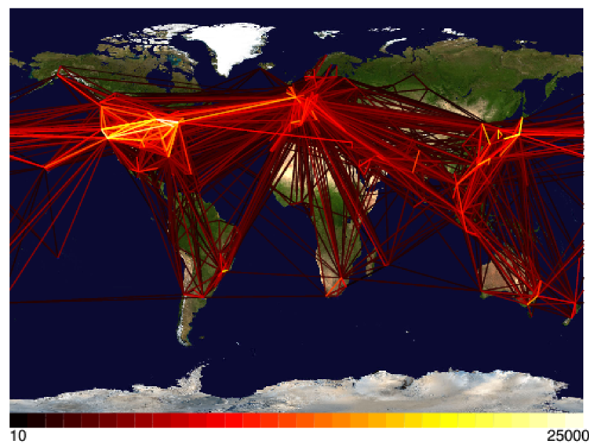
Figure 1: Global aviation network. A geographical representation of the civil aviation traffic among the $500$ largest international airports in over $100$ different countries is shown. Each line represents a direct connection between airports. The color encodes the number of passengers per day (see color code at the bottom) traveling between two airports. The network accounts for more than $95\%$ of the international civil aviation traffic. For each pair $(i,j)$ of airports, we checked all flights departing from airport $j$ and arriving at airport $i$. The amount of passengers carried by a specific flight within one week can be estimated by the size of the aircraft (We used manufacturer capacity information on over $150$ different aircraft types) times the number of days the flight operates in one week. The sum of all flights yields the passengers per week, i.e. $M_{ij}$ in Eq. (7). We computed the total passenger capacity $\sum M_{ij}$ of each airport $j$ per week and found very good agreement with independently obtained airport capacities.

Here we focus on mechanisms of the worldwide spreading of infectious diseases. Our model consists of two parts: a local infection dynamics and the global traveling dynamics of individuals similar to the models investigated in Longini (1985). However, both constituents of our model are treated on a stochastic level, taking full account of fluctuations of disease transmission, latency and recovery on one hand, and fluctuations of the geographical dispersal of individuals on the other. Furthermore we incorporate nearly the entire civil aviation network.

II Local Infection Dynamics

In the standard deterministic SIR model for infectious diseases, a population with $N$ individuals is categorized according to its infection status: susceptibles ($S$), infectious ($I$) or recovered and immune ($R$)Murray (1993); Anderson and May (1991). The dynamics which specifies the flow among these categories is given by

$$\text{d}s/\text{d}t=-\alpha\,s\,j,\qquad\text{d}j/\text{d}t=\alpha\,s\,j-\beta\,j\quad,$$ (1)

where $s=S/N$ and $j=I/N$ denote the relative number of susceptibles and infecteds, respectively. The relative number of recovered individuals $r=R/N$ is obtained by conservation of the entire population, i.e. $r(t)=1-j(t)-s(t)$, and $\tau=\beta^{-1}$ is the average infectious period. The key quantity describing the infection is the basic reproduction number $\rho_{0}=\alpha/\beta$, which is the average number of secondary infections transmitted by an infectious individual in an otherwise uninfected population. If $\rho_{0}>1$ and the initial relative number of susceptibles is greater than a critical value $s_{c}=1/\rho_{0}$ an epidemic develops ($\text{d}j/\text{d}t>0$). As the number of infected individuals increases, the fraction of susceptibles $s$ decreases and thus the number of contacts of infected individuals withfig susceptibles decreases until $s=s_{c}$ when the epidemic reaches its maximum and subsequently decays.

The above SIR model incorporates the underlying mechanism of transmission and recovery dynamics and has been able to account for experimental data in a number of cases. However, transmission of and recovery from an infection are intrinsically stochastic processes and the deterministic SIR model does not account for fluctuations. These fluctuations are particularly important at the beginning of an epidemic when the number of infecteds is very small.

In this regime a probabilistic description must be used. Schematically the stochastic infection dynamics is given by

$$S+I\xrightarrow{\alpha}2\,I,\qquad I\xrightarrow{\beta}\emptyset\quad.$$ (2)

The first reaction reflects the fact that an encounter of an infected individual with a susceptible results in two infecteds at a probability rate $\alpha$, the second indicates that infecteds are removed (recover) at a rate $\beta$ and effectively disappear from the population. The quantity of interest is the probability $p(S,I;t)$ of finding a number $S$ of susceptibles and $I$ infecteds in a population of size $N$ at time $t$. Assuming that the process is Markovian on the relevant time scales, the dynamics of this probability is governed by the master equation Gardiner (1985)

$$\partial_{t}\,p(S,I;t) = \frac{\alpha}{N}(S+1)\,(I-1)\,p(S+1,I-1;t)+\beta\,(I+1)\,p(S,I+1;t)$$ (3)

$$- \left(\frac{\alpha}{N}SI\,p-\beta\,I\right)p(S,I;t)\quad.$$

In addition to this dynamics one must specify the initial condition $p(S,I;\,t=t_{0})$ which is typically assumed to be a small but fixed number of infecteds $I_{0}$, i.e. $p(S,I;t=t_{0})=\delta_{I,I_{0}}\delta_{S,N-I_{0}}$.

The relation of the probabilistic master equation (3) to the deterministic SIR-model (1) can be made in the limit of a large but finite population, i.e. $N\gg 1$. In this limit one can approximate the master equation by a Fokker-Planck equation by means of an expansion in terms of conditional moments (Kramers-Moyal expansion Gardiner (1985)), see the supplement material. The associated description in terms of stochastic Langevin equations reads

$$\text{d}s/\text{d}t = -\alpha\,s\,j+\frac{1}{\sqrt{N}}\sqrt{\alpha\,s\,j}\xi_{1}(t)$$ (4)

$$\text{d}j/\text{d}t = \alpha s\,j-\beta\,j-\frac{1}{\sqrt{N}}\sqrt{\alpha\,s\,j}\xi_{1}(t)+\frac{1}{\sqrt{N}}\sqrt{\beta\,j}\xi_{2}(t)$$ (5)

Here, the independent Gaussian white noise forces $\xi_{1}(t)$ and $\xi_{2}(t)$ reflect the fluctuations of transmission and recovery, respectively. Note that the magnitude of the fluctuations are $\propto 1/\sqrt{N}$ and disappear in the limit $N\rightarrow\infty$ in which case Eqs. (1) are recovered. However, for large but finite $N$ a crucial difference is apparent: Eqs. (4) and (5) contain fluctuating forces and $N$ is a parameter of the system. A careful analysis shows that even for very large populations (i.e. $N\gg 1$) fluctuations play a prominent role in the initial phase of an epidemic outbreak and cannot be neglected. For instance even when $\rho_{0}>0$, a small initial number of infecteds in a population may no necessarily lead to an outbreak which cannot be accounted for by the deterministic model.

III Dispersal on the Aviation Network

As individuals travel around the world, the disease may spread from one place to another. In order to quantify the traveling behavior of individuals, we have analyzed all national and international civil flights among the $500$ largest airports by passenger capacity. This analysis yields the global aviation network shown in Fig. 1, further details of the data collection is compiled in the supplement material. The strength of a connection between two airports is given by the passengers capacity, i.e. the number of passengers that travel this route per day.

We incorporate the global dispersion of individuals into our model by dividing the population into $M$ local urban populations labeled $i$ containing $N_{i}$ individuals. For each $i$ the number of susceptibles, infecteds individuals is given by $S_{i}$ and $I_{i}$, respectively. In each urban area the infection dynamics is governed by the master equation (3).

Stochastic dispersal of individuals is defined by a matrix $\gamma_{ij}$ of transition probability rates between populations

$$S_{i}\xrightarrow{\gamma_{ij}}S_{j}\qquad I_{i}\xrightarrow{\gamma_{ij}}I_{j},\qquad i,j=1,...,M\quad,$$ (6)

where $\gamma_{ii}=0$. Along the same lines as presented above one can formulate a master equation for the pair of vectors $\mathbf{X}=\left\{S_{1},I_{1},...,S_{M},I_{M}\right\}$ which defines the stochastic state of the system. This master equation is provided explicitely in supplement material.

In order to account for the global spread of an epidemic via the aviation network one needs to specify the matrix $\gamma_{ij}$. Since the global exchange of individuals between urban areas is carried out by airborne travel one can estimate the probability rate matrix $\gamma_{ij}$ by t. We assume that an individual remains in urban area for some time before traveling to another region. A flight $j\rightarrow i$ is chosen according to the weights

$$w_{ij}=M_{ij}/\sum_{i}M_{ij}\quad.$$ (7)

where $M_{ij}$ is the number of passengers per unit time that depart from an airport in region $j$ and arrive at airport in region $i$. The matrix $w$ accounts for the overall connectivity of the aviation network as well as for the heterogeneity in the strength of the connections. Denoting the typical time period individuals remain at $i$ by $\tau_{i}$ the matrix $\gamma_{ij}$ is expressed in terms of $w_{ij}$ according to $\gamma_{ij}=w_{ij}/\tau_{j}$. If we assume that each airport is surrounded by a catchment area with a population $N_{i}$ the typical time individuals remain at $i$ is given by $\tau_{i}=N_{i}/\sum_{j}M_{ji}$. If the capacity of airport $i$ reflects the need of the associated catchment area (i.e. $N_{i}\propto\sum_{j}M_{ji}$), the waiting times $\tau_{i}$ are identical for all $i$, i.e. $\tau_{i}=\tau=\gamma^{-1}$ which implies $\gamma_{ij}=\gamma\,w_{ij}$. In our model the global rate $\gamma$ is a free parameter. In order to verify the its validity, we apply our model to the SARS outbreak. The rate $\gamma$ can be computed from the ratio of the number of infected individuals in Hong Kong to the number of infected individuals outside Hong Kong, which is provided by the WHO data. For the local infection dynamics we use a simple extension of the above stochastic SIR model: The categories $S$, $I$ and $R$ are completed by a category $L$ of latent individuals which have been infected but are not infectious yet themselves, accounting for the latency of the disease. In our simulations individuals remain in the latent or infectious stage for periods drawn from the delay distribution provided in Fig. 2 in Donnelly et al. (2003). In our simulation we chose random infection times the distribution of which is known for SARS Donnelly et al. (2003). In a realistic simulation the basic reproduction number $\rho_{0}$ cannot be assumed to be constant over time. Successful control measures, for instance, generally decrease $\rho_{0}$. We chose a time dependent $\rho_{0}(t)$ as provided by Refs. Riley et al. (2003); Lipsitch et al. (2003).

IV Results of Simulations

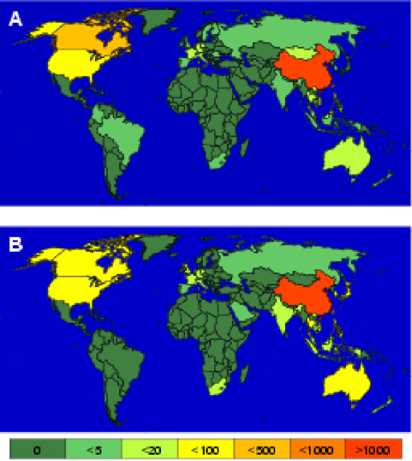
Figure 2: (a) Geographical representation of the global spreading of probable SARS cases on May 30th, 2003 as reported by the WHO and CDC. The first cases of SARS emerged in mid November 2002 in Guangdong Province, ChinaCDC (2003). The disease was then carried to Hong Kong on the February 21st, 2003 and began spreading around the world along international air travel routes, as tourists and the medical doctors who treated the early cases traveled internationally. As the disease moved out of southern China, the first hot zones of SARS were Hong Kong, Singapore, Hanoi (Viet Nam) and Toronto (Canada), but soon cases in Taiwan, Thailand, the United States, Europe and elsewhere were reported. (a) Geographical representation of the results of our simulations 90 days after an initial infection in Hong Kong, The simulation corresponds to the real SARS infection at the end of May, 2003. Since our Since the simulations cannot describe the infection in China, where the disease started in November 2002, we used the WHO data for China.

Fig. 2 depicts a geographical representation of the results of our simulations. Initially, an infected individual was placed in Hong Kong. For this initial condition we simulated $1000$ realizations of the stochastic model and computed the mean value $\left\langle I(t)\right\rangle$ of the number of infecteds at each node $i=1,...,M$ of the network. Since the size of catchment areas varies on many scales, the fluctuation range is best quantied by the means of the relative variance of $z=\log\,I$, i.e. $\eta=\sqrt{\left\langle z^{2}\right\rangle-\left\langle z\right\rangle^{2}}/<z>.$ In our simulations we computed this measure for every $i$ of the network. Fig 2 shows the prediction of our model for the spread of SARS at $t=90$ days after the initial outbreak in Hong Kong (February 19, 2003), corresponding to the May 20, 2003. The results of our simulations are in remarkable agreement with the worldwide spreading of SARS as reported by the WHO (compare Fig. 2): There is an almost one-to-one correspondence between infected countries as predicted by the simulations and the WHO data.

Country	WHO	WHO	Simulation
	05/20/2003	05/30/2003	Average	$\eta$	Min	Max
Hong Kong	1718	1739	1951	0.35	1373.9	2770.4
Taiwan	383	676	318.2	0.55	184.0	550.3
Singapore	206	206	136.6	0.68	69.4	268.7
Japan	-	-	60.4	0.84	26.6	137.0
Canada	140	188	41.8	0.94	16.4	106.6
USA	67	66	65.9	0.84	28.4	152.7
Vietnam	63	63	49.2	0.86	20.7	116.3
Philippines	12	12	30.0	0.97	6.2	50.7
Germany	9	10	14.4	1.1	4.8	43.1
Netherlands	-	-	5.9	1.09	2.0	17.6
Bangladesh	-	-	10	1.15	3.2	31.6
Mongolia	9	9	-	-	-	-
Italy	9	9	5.3	1.02	1.9	14.6
Thailand	8	8	35.4	0.89	14.5	86.8
France	7	7	7.6	1.09	2.6	22.6
Australia	6	6	27.0	1.05	10.1	72.5
Malaysia	7	5	17.7	1.05	6.2	50.7
United Kingdom	4	4	16.7	1.04	5.9	47.0

Table 1: A comparison of the SARS case reports provided by the WHO and the results of our simulation for all countries with a reported case number $\geq 4$. The expected number of infecteds predicted by our model is estimated by the average over $1000$ realizations of the stochastic model. The epidemic was simulation for $t=90$ days after the initial outbreak of SARS in Hong Kong (February 19, 2003), yielding a simulation end of May 20, 2003. The range defined by column $6$ and $7$ was computed by means of the fluctuation measure $\eta$ (see text) which is approximately one for all countries.

Also the orders of magnitude of the numbers of infected individuals in a country agree (Table 1). While for most countries the reported cases by the WHO lie within the fluctuation range, two deviation between the reported cases and the predictions of the simulation are apparent: Our simulations predict a relatively high number of SARS cases in Japan (between 26.6 and 137.0). However, the Japanese Government reported no confirmed case (only 5 suspected cases) of SARS in Japan, as of May 30, 2003. How a single realization may deviate from the expectation can be seen from the difference between the simulation and the reported cases in the USA and Canada. The simulations show that on average the USA should have a higher number of SARS cases than Canada, although the opposite was reported by the WHO. The impact of the inherent stochasticity of the infection and traveling dynamics is discussed in the next section.

V The impact of fluctuations

Figure 3: Two confined populations with exchange of individuals. In each population the dynamics is governed by the SIR-reaction scheme (6). Individuals travel from on population to the other at a rate $\gamma$. Parameters are $N_{A}=N_{B}=10,000$, $R_{0}=4$ and an initial number of infecteds $I_{0}=20$ in population $A$ Left: The probability $p(\gamma)$ of an outbreak occurring in population $B$ as a function of transition rate $\gamma$. The insets depict histograms of the time lag $T$ between the outbreaks in $A$ and $B$ for those realization for which an outbreak occurs in $B$. The circles are results of the simulations of $100,000$ realizations, the solid curve is the analytic result of Eq. (8) Right: A star-shaped network with a central population $A$ connected to $M-1$ populations $B_{1},...,B_{M-1}$with rates $\gamma_{1},...,\gamma_{M-1}$. The cumulated variance (Eq. LABEL:eq:typicalvariance) for a star network with 32 populations is depicted as a function of the average transmission rate $\bar{\gamma}$. Two cases are exemplified: equal rates (circles) and distributed rates according to Eq. 10 with $\gamma_{{\rm max}}/\gamma_{{\rm min}}\approx 1000$ (squares). The solid lines show the analytical results given by Eq. 9 and Eq. 8. Parameters are $N_{A}=N_{B}=10,000$, $R_{0}=4$ and an initial number of infecteds $I_{0}=20$ in population $A$. The numerical values are obtained by calculating the variance of the fluctuations of 100 different realizations of the epidemic outbreak for each $\bar{\gamma}$.

Bearing in mind the low number of infections and the small value of $\rho_{0}$ for SARS, the high degree of predictability, i.e. the low impact of fluctuations on the network level, is rather surprising, especially because our simulations take into account the full spectrum of fluctuations of disease transmission, recovery and dispersal and that the system evolves on a highly complex network. Naively, one expects that dispersal fluctuations between two given populations are amplified as the epidemic spreads globally and that no prediction can be made. In order to clarify this important point, consider the system of two confined populations $A$ and $B$ which exchange individuals as depicted in Fig. 3. For simplicity we assume that both populations have the same size (i.e. $N_{A}=N_{B}=N$) and individuals traverse at a rate $\gamma$. Now assume that initially a small number of infected $I_{0}$ is introduced to population $A$ without any infecteds contained in $B$. For a sufficiently high number of infecteds in $A$ an epidemic occurs. For $\gamma>0$ infecteds are introduced to $B$ and a subsequent outbreak may occur in $B$ after a time lag $T$. Fig. 3 depicts the results of simulations for two populations with $N=10,000$ and $\rho_{0}=4$. Various realizations of the time course $I_{A}(t)$ and $I_{B}(t)$ of the epidemic in both populations we computed. The initial number of infecteds in population was $I_{A}(t=0)=I_{0}=20$. The left panel depicts the probability $p(\gamma)$ of an outbreak occuring in population $B$ as a function if the transition rate $\gamma$. For large enough rates the probability is nearly unity, since a sufficient number of infecteds is introduced to $B$. For very low rates $\gamma$ no infecteds are introduced to $B$ during the time span of the epidemic in $A$ and thus $p(\gamma)\rightarrow 0$ as $\gamma\rightarrow 0$. For intermediate values of $\gamma$ the probability $p(\gamma)$ is neither one nor unity and the time course in population $B$ cannot be predicted with certainty. The function $p(\gamma)$ is given by

$$p(\gamma)=1-\exp(-\gamma/\gamma^{\star}),$$ (8)

where the critical rate $\gamma^{\star}$ is a function of the parameters $\rho_{0}$ and $N$. The insets depict histograms of the time lag $T$ for those realization for which an outbreak occured in $B$. Each histogram corresponds to a different transition rate $\gamma$. The smaller $\gamma$ the higher the variability in $T$. Note that even in a range in which $p(\gamma)\approx 1$, the time lag $T$ is still a stochastic quantity with a high degree of variance (see also the supplement material).

Consequently, the introduction of stochastic exchange of infected individuals leads to a lack of predictability in the time of onset of the initially uninfected population. In the light of the analysis of two populations, the predictability in the case of SARS on the aviation network seems even more puzzling.

The situation changes drastically in networks which exhibits a high degree of variability in the rate matrix $\gamma_{ij}$. Clearly, this is the case for the aviation network. Consider the simple network depicted in Fig. 3. Each population contains $N$ individuals. A central population $A$ is coupled to a set of $M-1$ surrounding populations $B_{1},...B_{M-1}$. Assume that initially a number of infecteds $I_{0}$ is introduced to the central population $A$ such that an outbreak occurs. The entire set of rates $\left\{\gamma_{j}\right\}{}_{j=1,...,M-1}$ determines the behaviour in the surrounding populations. If all rates $\gamma_{j}$ are identical and very small we expect no infection to occur in the $B_{j}$, for large enough $\gamma_{j}$ an outbreak will occur in every $B_{j}$. In the aviation network, however, transition rates are distributed on many scales and the response of the network to a central outbreak depends on the statistical properties of this distribution denoted by$q(\gamma)$. In order to quantify the reaction of the network we introduce for each surrounding population a binary number $\xi_{j}$ with $j=1,...,M-1$ which is unity if an outbreak occurs in $B_{j}$ and zero if it doesn’t. According to Eq. (8) for a given rate $\gamma$ this quantity is a random number with a conditional probability density $p(\xi_{i}|\gamma)=(1-p(\gamma))\,\delta(\xi_{i})+p(\gamma)\,\delta(\xi_{i}-1)$. The variability of the network is thence quantified be the cumulative variance per population and we define

$$\sigma=\frac{4}{M-1}\sum_{i}\text{var}(\xi_{i})=\int\text{d}\gamma\,p(\gamma)\,(1-p(\gamma))\,q(\gamma)$$ (9)

as a measure for the uncertainty of the network response. If for example $q(\gamma)=\delta(\gamma-\bar{\gamma})$, i.e. all transition rate are identical and equal to $\bar{\gamma}$, then $\sigma(\bar{\gamma})=4\,p(\bar{\gamma})(1-p(\bar{\gamma})$, which is unity for $p(\bar{\gamma})=1/2$. Comparing with Eq. (8) we see that when $\bar{\gamma=\gamma^{\star}\log 2}$ the system with identical transition rates $\gamma_{i}=\bar{\gamma}$ exhibits the highest degree of unpredictability when the rates are of the order of the critical rate defined by (8). The function $\sigma(\bar{\gamma})$ is shown in Fig. 3.

Now assume that the rate $\gamma_{j}$ are drawn from a distribution

$$q(\gamma)=\frac{1}{\log(\gamma_{\text{max}}/\gamma_{\min})}\frac{1}{\gamma}\qquad\gamma_{\text{max}}\leq\gamma\leq\gamma_{\min}.$$ (10)

which implies a high degree of variance within the interval $\left[\gamma_{\text{min}},\gamma_{\text{max}}\right]$ (i.e. $\gamma_{j}$ is distributed uniformly on a logarithmic scale). This high variability in rates drastically changes the predictability of the system. Inserting into Eq. (9) yields $\sigma(\bar{\gamma})$ for strongly distributed rates. In Fig. 3 this function is compared to a system of identical transition rates. On one hand, for intermediate values of $\gamma\approx\gamma^{\star}$ the predictability is much higher than in the system of identical rates. This is a rather counterintuitive result. Despite the additional randomness in transition rates, the degree of determinism is increased.

VI Control Strategies

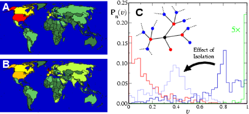
Figure 4: Left: Geographical representation of the results two simulations of hypothetical SARS outbreaks 90 days after an initial infection in (a) New York and (b) London for the same parameters and color code as in Fig. 2. Right: Impact and control of epidemics. The probability $p_{n}(v)$ of having to vaccinate a fraction $v$ of the population in order to prevent the epidemic from spreading, if an initial infected individual is permitted to travel $n=1$ (red), $2$ (blue), and $3$ (green) times. The probability $p_{n}(v)$ is estimated by placing the infected individual on a node $i$ (black dot) of the network. The fraction $v_{i}$ associated with node $i$ is given by the number of susceptibles in a subnetwork which can be reached by the infected individual after $n=1,\,2$ and $3$ steps. Histogramming $v_{i}$ for all nodes $i$ yields an estimate for $p_{n}(v)$. The light-blue curve depicts the strong impact of isolating only $2\%$ of the largest cities after an initial outbreak ($n=2$) and is to be compared to the blue curve.

Fig. 4 exemplify how our model can be employed to predict endangered regions if the origin of a future epidemic is located quickly. The figure depict simulations of the global spread of SARS at $t=90$ days after hypothetical outbreaks in New York and London, respectively. Despite the worldwide spread of the epidemic in each case, the degree of infection of each country differs considerably, which has important consequences for control strategies.

Vaccination of a fraction of the population reduces the fraction of susceptibles and thus yields a smaller effective reproduction number $\rho$. If a sufficiently large fraction is vaccinated, $\rho$ drops below 1 and the epidemic becomes extinct. The global aviation network can be employed to estimate the fraction of the global population that needs to be vaccinated in order to prevent the epidemic from spreading. Fig. 4 demonstrates that a quick response to an initial outbreak is necessary if global vaccination is to be avoided. The Figure depicts the probability $p_{n}(v)$ of having to vaccinate a fraction $v$ of the population if an infected individual is randomly placed in one of the cities and permitted to travel $n=1,\,2$ or $3$ times. For the majority of originating cities the initial spread is regionally confined and thus a quick response to an outbreak requires only a vaccination of a small fraction of the population. However, if the infected individual travels twice, the expected fraction $\left\langle v\right\rangle$ of the population which needs to be vaccinated is considerable ($74.58\%$). For $n=3$ global vaccination is necessary.

As a reaction to a new epidemic outbreak, it might be advantageous to impose travel restrictions to inhibit the spread. Here we compare two strategies: (i) the shutdown of individual connections and (ii) the isolations of cities. Our simulations show that an isolation of only $2\%$ of the largest cities already drastically reduces $\left\langle v\right\rangle$ (with $n=2$) from $74.58\%$ to $37.50\%$ (compare the blue and light-blue curves in Fig. 4). In contrast, a shutdown of the strongest connections in the network is not nearly as effective. In order to obtain a similar reduction of $\left\langle v\right\rangle$ the top $27.5\%$ of connections would need to be taken off the network. Thus, our analysis shows that a remarkable success is guaranteed if the largest cities are isolated as a response to an outbreak.

In a globalized world with millions of passengers traveling around the world week by week infectious diseases may spread rapidly around the world. We believe that a detailed analysis of the aviation network represents a cornerstone for the development of efficient quarantine strategies to prevent diseases from spreading. As our model is based on a microscopic description of traveling individuals our approach may be considered a reference point for the development and simulation of control strategies for future epidemics.

We thank E. Bodenschatz for critical reading of the manuscript and stimulating discussions. This research was supported in part by the National Science Foundation under Grant No. PHY99-07949.

References

- Bernoulli (1760) D. Bernoulli, Mém. Math. Phys. Acad. Roy. Sci., Paris p. 1 (1760).
- Keeling et al. (2001) M. J. Keeling, M. E. J. Woolhouse, D. J. Shaw, L. Matthews, M. Chase-Topping, D. T. Haydon, S. J. Cornell, J. Kappey, J. Wilesmith, and B. T. Grenfell, Science 294, 813 (2001).
- Smith et al. (2002) D. L. Smith, B. Lucey, L. A. Waller, J. E. Childs, and L. A. Real, Proc. Natl. Acam. Sci. USA 99, 3668 (2002).
- Keeling et al. (2003) M. J. Keeling, M. E. J. Woolhouse, R. M. May, G. Davies, and B. T. Grenfell, Nature 421, 136 (2003).
- Bullock et al. (2002) J. M. Bullock, R. E. Kenward, and R. S. Hails, eds., Dispersal Ecology, The 42nd Symposium of the British Ecological Society held at the University of Reading (Blackwell Publishing, United Kingdom, 2002).
- Murray (1993) J. D. Murray, Mathematical Biology (Springer-Verlag Berlin Heidelberg New York, 1993).
- Langer (1964) W. L. Langer, Scientific American 2, 114 (1964).
- Noble (1974) J. V. Noble, Nature 250, 726 (1974).
- Grenfell et al. (2001) B. T. Grenfell, O. N. Bjornstadt, and J. Kappey, Nature 414, 716 (2001).
- Mollison (1991) D. Mollison, Math. Biosci. 107, 255 (1991).
- Longini (1985) L. A. R. I. M. Longini, Mathematical Biosciences 75, 3 (1985).
- Anderson and May (1991) R. M. Anderson and R. M. May, Infectious Diseases of Humans (Oxford Univ. Press, Oxford, 1991).
- Gardiner (1985) C. W. Gardiner, Handbook of Stochastic Methods (Springer Verlag, Berlin, 1985).
- Donnelly et al. (2003) C. A. Donnelly, A. C. Ghani, G. M. Leung, A. J. Hedley, C. Fraser, S. Riley, L. J. Abu-Raddad, L.-M. Ho, T.-Q. Thach, P. Chau, et al., Lancet 361, 1761 (2003).
- Riley et al. (2003) S. Riley, C. Fraser, C. A. Donnelly, A. C. Ghani, L. J. Abu-Raddad, A. J. Hedley, G. M. Leung, L.-M. Ho, T.-H. Lam, T. Q. Thach, et al., Science 300, 1961 (2003).
- Lipsitch et al. (2003) M. Lipsitch, T. Cohen, B. Cooper, J. M. Robins, S. Ma, L. James, G. Gopalakrishna, S. K. Chew, C. C. Tan, M. H. Samore, et al., Science 300, 1966 (2003).
- CDC (2003) CDC, Morb Mortal Wkly Rep 52, 241 (2003).