Production of three-body Efimov molecules in an optical lattice

Abstract

We study the possibility of associating meta-stable Efimov trimers from three free Bose atoms in a tight trap realised, for instance, via an optical lattice site or a microchip. The suggested scheme for the production of these molecules is based on magnetically tunable Feshbach resonances and takes advantage of the Efimov effect in three-body energy spectra. Our predictions on the energy levels and wave functions of three pairwise interacting ⁸⁵Rb atoms rely upon exact solutions of the Faddeev equations and include the tightly confining potential of an isotropic harmonic atom trap. The magnetic field dependence of these energy levels indicates that it is the lowest energetic Efimov trimer state that can be associated in an adiabatic sweep of the field strength. We show that the binding energies and spatial extents of the trimer molecules produced are comparable, in their magnitudes, to those of the associated diatomic Feshbach molecule. The three-body molecular state follows Efimov’s scenario when the pairwise attraction of the atoms is strengthened by tuning the magnetic field strength.

I Introduction

Since the early days of quantum mechanics, the understanding of the complexity of few-body energy spectra has been the subject of numerous theoretical and experimental studies. Already in 1935 Thomas Thomas35 predicted that three particles may be rather tightly bound even when their short ranged pairwise interactions support only a single, arbitrarily weakly bound state. The energy of the tightly bound three-body state was found to diverge in the hypothetical limit of a zero range binary potential. Thomas’ discoveries were later generalised by Efimov Efimov70 , predicting that the number of bound states of three identical Bosons increases beyond all limits when the pairwise attraction between the particles is weakened in such a way that the only two-body bound state ceases to exist. Such an excited three-body energy state that appears under weakening of the attractive pairwise interaction is called an Efimov state. Conversely, under strengthening of the attractive part of the binary potential an Efimov state disappears into the continuum. This remarkable quantum phenomenon of three-body energy spectra is usually referred to as Efimov’s scenario.

The existence of Efimov states in nature has still not been finally confirmed. Likely candidates may be found among the systems of identical Bosons, whose binary interaction potential supports only a single, weakly bound state. Already in 1977 Lim et al. Lim77 predicted the existence of an excited state of the helium trimer molecule ⁴He₃ which followed Efimov’s scenario. This discovery has later been confirmed by independent theoretical studies Cornelius86 ; Esry96 ; Kolganova98 ; Nielsen98 ; Gonzalez99 ; Blume00 ; Barletta01 ; Jensen04 using more accurate helium dimer potentials. From the experimental viewpoint, the observations of Ref. Grisenti00 clearly reveal that the helium dimer ⁴He₂ is indeed weakly bound. Even the helium trimer molecule has been detected by diffracting a helium molecular beam Schoellkopf94 from a micro-fabricated material transmission grating. While state selective diffraction experiments with helium trimers may, in principle, be possible HK00 , there is still no conclusive evidence for the existence of their exited state.

The possibility of manipulating the low energy inter-atomic interactions, using magnetically tunable Feshbach resonances, has provided new perspectives for the observation of Efimov’s effect. Recent experiments with cold gases of Fermionic atoms Regal03 ; Strecker03 as well as Bosonic species Herbig03 ; Duerr04 ; Xu03 ; Thompson04 have demonstrated that adiabatic sweeps of the magnetic field strength can be used to associate highly excited diatomic Feshbach molecules with an arbitrarily weak bond. While all these experiments were performed in atom traps under comparatively weak spatial confinement, there have been suggestions to produce molecules in the tightly confining light potential of an optical lattice Jaksch02 . Since tight lattices suppress number fluctuations between different sites Greiner02 , the molecular association may, in principle, be performed with two or even three atoms per site. A similarly tight or even stronger harmonic confinement of atoms may be achieved in microchip traps Long03 . The energy levels of a pair of interacting atoms in a tight micro-trap have been determined in Refs. BERW_FP28 ; Tiesinga00 ; Bolda02 . The universal properties Yamashita03 ; Braaten04 of three-body energy spectra in the presence of a confining harmonic potential have been studied in Ref. Jonsell02 , using an adiabatic approximation to solve the stationary Schödinger equation in hyper-spherical coordinates Blume02 .

In this paper we exactly solve the Faddeev equations F_JETP12 to determine the magnetic field dependence of the energy levels of three identical Bose atoms, whose pairwise interactions are tuned, using the technique of Feshbach resonances, in a harmonic micro-trap realised by an optical lattice site or a microchip. Our results show that linear sweeps of the magnetic field strength can be used to populate the lowest energetic meta-stable Efimov trimer molecular state, largely in analogy to the association of diatomic Feshbach molecules. We show that the properties of the trimers produced, with respect to the strength of their bonds, are comparable to those of the associated diatomic Feshbach molecule. We illustrate all our general findings for the example of the 155 G Feshbach resonance of ⁸⁵Rb Bose atoms.

The paper is organised as follows: In Section II we discuss those universal properties of near resonant diatomic bound states that are crucial for the association of Efimov trimers. We then introduce the particular requirements on the type of Feshbach resonance, under which universality can be attained over a wide range of magnetic field strengths. Our results indicate that broad, entrance channel dominated Feshbach resonances may be best suited to produce the trimers and preserve their stability on time scales sufficiently long to study their properties. We provide a general criterion that shows why the 155 G resonance of ⁸⁵Rb meets these requirements KGB03 ; KGG04 ; Marcelis04 .

In Section III we first illustrate the occurrence of the Thomas and Efimov effects in the energy spectra of three Bose atoms in free space, whose binary interactions are tuned using the technique of Feshbach resonances. Our discussion reveals, in particular, why all Efimov trimer states in such systems are, in general, intrinsically meta-stable. We then show how the three-body energy spectrum is modified due to the presence of the harmonic confining potential of an isotropic atom trap. These considerations allow us to identify the lowest energetic Efimov state as the molecular trimer state that can be associated in an adiabatic sweep of the magnetic field strength.

Section IV illustrates the energy levels and wave functions of three ⁸⁵Rb atoms under the tight confinement of an optical lattice site or a microchip trap. We show that, under realistic conditions, the trimer molecules produced, when released from the lattice, are sufficiently confined in space that they can be identified as separate entities of a dilute gas. We then suggest a general scheme for their detection that directly takes advantage of the periodic nature of an optical lattice.

All the details of our calculations are given in the appendices: Appendix A introduces the separable binary potential L_PR135 ; Sandhas72 ; Beliaev90 that we have used to accurately describe the low energy scattering properties of a pair of ⁸⁵Rb atoms. We show, furthermore, how the separable potential approach can be extended to determine the two-body energy levels, in the presence of an isotropic harmonic atom trap, over a wide range of trap frequencies. We apply these techniques in Appendix B to derive a general scheme to exactly solve the Faddeev equations for three pairwise interacting atoms including the confining trapping potential. Since our approach differs considerably from the known techniques for the solution of the Faddeev equations in free space, we provide a detailed description of their numerical implementation. To demonstrate its predictive power with respect to three-body energy spectra, we provide estimates of the accuracy of our separable potential approach through comparisons with ab initio calculations Barletta01 of the helium trimer ground and excited state energies.

II Energy levels of a trapped atom pair

In this section we introduce the concept of universal two-body scattering and bound state properties characteristic for cold collision physics in the vicinity of zero energy resonances. These universal properties are crucial for the existence of the Thomas and Efimov effects in three-body energy spectra. We describe the conditions under which the universality of binary physical observables can be attained over a wide range of magnetic field strengths in experiments using Feshbach resonances to tune the inter-atomic interactions. We provide the relevant physical parameters of the microscopic binary potential that determine the energy spectra of an atom pair in free space as well as under the spatial confinement of an atom trap. We then show how the variation of the energies under adiabatic changes of the magnetic field strength can be used to associate diatomic molecules. Throughout this paper we discuss applications for the example of the 155 G Feshbach resonance of ⁸⁵Rb ($1\,\mathrm{G}=10^{-4}$ T). The underlying physical concepts, however, are quite general and can be applied to cold collisions of other species of Bose atoms involving what we shall identify as entrance channel dominated resonances.

II.1 Resonance enhanced scattering

II.1.1 Magnetic field tunable Feshbach resonances

Binary collisions in cold gases involve large de Broglie wavelengths which typically very much exceed all length scales set by the inter-atomic interactions. At the low collision energies the microscopic potential enters the description of scattering phenomena only in terms of a single length scale, the $s$ wave scattering length $a$. The experimental technique of Feshbach resonances employs a homogeneous magnetic field of strength $B$ to manipulate the scattering length, taking advantage of the fact that the pairwise interaction depends on the coupling between the atomic Zeeman levels. Each Zeeman state is determined by the pair of total angular momentum quantum numbers $(f,m_{f})$ of the hyperfine level with which the Zeeman state correlates adiabatically at zero magnetic field. In our applications to cold gases of ⁸⁵Rb the atoms are prepared in the magnetically trapped hyperfine state with the total angular momentum quantum number $f=2$ and the orientation quantum number $m_{f}=-2$ with respect to the direction of the magnetic field. The interaction between the atoms is usually described in terms of the binary scattering channels associated with the pairs of Zeeman levels of the individual atoms. The relative energies between the dissociation thresholds associated with the channels can be tuned using the Zeeman effect. We shall denote the open $s$ wave channel of a pair of asymptotically separated atoms of the gas as the entrance channel.

The typically weak inter-channel coupling can be grossly enhanced by tuning the energy $E_{\mathrm{res}}(B)$ of a closed channel vibrational state $|\psi_{\mathrm{res}}\rangle$ (the Feshbach resonance level) in the vicinity of the dissociation threshold of the entrance channel. General considerations Mies00 ; GKGTJ_JPB37 show that a virtual energy match between $E_{\mathrm{res}}(B)$ and the threshold leads to a zero energy resonance in the entrance channel, i.e. a singularity of the scattering length, described by the formula:

$$a=a_{\mathrm{bg}}\left(1-\frac{\Delta B}{B-B_{0}}\right).$$ (1)

Here $a_{\mathrm{bg}}$ is usually referred to as the background scattering length, $\Delta B$ is the resonance width and $B_{0}$ is the position of the zero energy resonance.

II.1.2 Universal properties of near resonant bound state wave functions

The emergence of the zero energy resonance indicates the degeneracy of the binding energy $E_{\mathrm{b}}(B)$ of the highest excited vibrational multi-channel molecular bound state $|\psi_{\mathrm{b}}\rangle$ (the Feshbach molecule) with the threshold for dissociation of the entrance channel at the magnetic field strength $B_{0}$. The magnetic field dependence of $E_{\mathrm{b}}(B)$ is due to the perturbation of the physically relevant multi-channel energy levels by the strong coupling between the entrance channel and the closed channel Feshbach resonance state. The energy $E_{\mathrm{b}}(B)$ approaches the entrance channel dissociation threshold from the side of positive scattering lengths, while beyond the resonant field strength $B_{0}$, at negative scattering lengths, the bound state $|\psi_{\mathrm{b}}\rangle$ is transferred into a virtual state. At magnetic field strengths in the close vicinity of the zero energy resonance, all low energy binary collision properties are thus dominated by the properties of the bound state $|\psi_{\mathrm{b}}\rangle$, whose wave function becomes universal in the limit $a\to\infty$. This implies that the admixture of the Feshbach resonance level to the molecular bound state $|\psi_{\mathrm{b}}\rangle$ vanishes in accordance with the following asymptotic formula GKGTJ_JPB37 :

$$|\langle\psi_{\mathrm{res}}|\psi_{\mathrm{b}}\rangle|^{2}\underset{a\to\infty}{\sim}1/\left(1+\frac{1}{2}\mu_{\mathrm{res}}\frac{a_{\mathrm{bg}}\Delta B}{a}\frac{ma^{2}}{\hbar^{2}}\right).$$ (2)

Here $\mu_{\mathrm{res}}=dE_{\mathrm{res}}/dB$ is the virtually constant magnetic moment of the resonance level $|\psi_{\mathrm{res}}\rangle$ and $m$ is the atomic mass. We note that, in general, the physically relevant Feshbach molecular state $|\psi_{\mathrm{b}}\rangle$ and the Feshbach resonance level $|\psi_{\mathrm{res}}\rangle$ are considerably different with respect to their magnetic moments and their spatial extents. The state $|\psi_{\mathrm{b}}\rangle$ binds the atoms, while $|\psi_{\mathrm{res}}\rangle$ may have only a short lifetime, in particular, when the inter-channel coupling is strong.

In the vicinity of the magnetic field strength $B_{0}$ the long range molecular bound state $|\psi_{\mathrm{b}}\rangle$ consists mainly of its component in the entrance channel, which is given by the usual form of a near resonant bound state wave function KGJB03 ; GKGTJ_JPB37 :

$$\psi_{\mathrm{b}}(r)\approx\frac{e^{-r/a}}{r\sqrt{2\pi a}}.$$ (3)

Its mean inter-atomic distance, i.e. the bond length, then diverges like the scattering length in accordance with the relationship:

$$\langle r\rangle=\int\ d^{3}r\ r\left|\psi_{\mathrm{b}}(r)\right|^{2}\approx a/2.$$ (4)

The associated binding energy is also determined solely in terms of the scattering length by the universal formula:

$$E_{\mathrm{b}}\approx-\hbar^{2}/(ma^{2}).$$ (5)

II.1.3 Entrance and closed channel dominated Feshbach resonances

The possibility of magnetically tuning the scattering length using Feshbach resonances is unique among all physical systems. The universal properties of the near resonant bound state wave function described by Eqs. (3), (4) and (5), however, are not directly related to the inter-channel coupling and apply equally well, for instance, also to the deuteron in nuclear physics BlattWeisskopf52 and to the weakly bound helium dimer ⁴He₂ van der Waals molecule Grisenti00 . Since our applications to the association of Efimov trimer molecules crucially depend on the single channel nature of the bound state $|\psi_{\mathrm{b}}\rangle$ of the Feshbach molecule, we shall briefly outline the requirements on the Feshbach resonance that assure the validity of the universal considerations over a significant range of magnetic field strengths. To this end, we consider the general properties of long range alkali van der Waals molecules that are determined, to an excellent approximation, by the scattering length in addition to the asymptotic form $-C_{6}/r^{6}$ of the binary potential at large inter-atomic distances $r$. In accordance with Ref. GF_PRA48 , we shall describe the dependence of the molecular energy level on the van der Waals dispersion coefficient $C_{6}$ in terms of a mean scattering length $\bar{a}$, which is given by the formula:

$$\bar{a}=\frac{l_{\mathrm{vdW}}}{\sqrt{2}}\ \frac{\Gamma(3/4)}{\Gamma(5/4)}.$$ (6)

Here $l_{\mathrm{vdW}}=\frac{1}{2}\left(mC_{6}/\hbar^{2}\right)^{1/4}$ is usually referred to as the van der Waals length and $\Gamma$ denotes Euler’s gamma function. The binding energy of an alkali van der Waals molecule is then determined by the formula GF_PRA48 :

$$E_{\mathrm{b}}=-\hbar^{2}/\left[m(a-\bar{a})^{2}\right].$$ (7)

As discussed in detail for the examples of ²³Na and ⁸⁵Rb in Ref. KGG04 , a variety of Feshbach resonances can be classified on the basis of the properties of their associated Feshbach molecules: Throughout this paper, we shall denote a Feshbach resonance as entrance channel dominated when the binding energy $E_{\mathrm{b}}(B)$ is well approximated by Eq. (7) in some range of magnetic field strengths about $B_{0}$, and, at the same time, the contribution of the mean scattering length $\bar{a}$ of Eq. (6) improves the universal estimate of Eq. (5), i.e.:

$$\left|E_{\mathrm{b}}+\frac{\hbar^{2}}{m(a-\bar{a})^{2}}\right|<\left|E_{\mathrm{b}}+\frac{\hbar^{2}}{ma^{2}}\right|.$$ (8)

The bound state $|\psi_{\mathrm{b}}\rangle$ then describes a van der Waals molecule which implies that its properties are determined mainly by the entrance channel potential rather than the resonance level. In fact, the general considerations of Ref. GKGTJ_JPB37 show that the admixture of the closed channel resonance state $|\psi_{\mathrm{res}}\rangle$ to the Feshbach molecular state $|\psi_{\mathrm{b}}\rangle$ is negligible as soon as Eq. (7) applies to its energy (cf., also, Fig. 3 of Ref. KGG04 ). A general criterion for the applicability of Eq. (7) can be derived from the two channel approach of Ref. GKGTJ_JPB37 which leads to the following inequality Petrov04FR :

$$\left|\frac{\bar{a}}{a_{\mathrm{bg}}}\frac{\hbar^{2}/(m\bar{a}^{2})}{\mu_{\mathrm{res}}\ \Delta B}\right|\ll 1.$$ (9)

Under the conditions of Eq. (9), the reason for the suppression of the closed channel contribution to the Feshbach molecule is the large detuning of the Feshbach resonance level from the dissociation threshold of the entrance channel at the position $B_{0}$ of the zero energy resonance GKGTJ_JPB37 . The parameters for the 155 G Feshbach resonance of ⁸⁵Rb, i.e. $\mu_{\mathrm{res}}/h=-3.12\,$MHz/G Kokkelmans_private04 , $C_{6}=4703\,$a.u. KKHV_PRL88 ($1\,\mathrm{a.u.}=0.095734\times 10^{-24}\,$J nm⁶), $\Delta B=10.71\,$G Claussen03 , and $a_{\mathrm{bg}}=-443\,a_{0}$ ($a_{0}=0.052918\,$nm) Claussen03 , give the quantity in Eq. (9) to be $4\times 10^{-2}$. The 155 G Feshbach resonance of ⁸⁵Rb is therefore entrance channel dominated. Similar conclusions were reached in Refs. KGB03 ; Marcelis04 .

There is also a variety of closed channel dominated Feshbach resonances, like, e.g., those in ²³Na KGG04 , whose Feshbach molecular states $|\psi_{\mathrm{b}}\rangle$ become universal [cf. Eq. (3)] only in a small region of magnetic field strengths about the zero energy resonance at $B_{0}$. These states are not intermediately transferred into a van der Waals molecule away from the resonance. Closed channel dominated resonances do not satisfy the criterion of Eq. (9) and the bound states $|\psi_{\mathrm{b}}\rangle$ are thus significantly influenced by the resonance level $|\psi_{\mathrm{res}}\rangle$ immediately outside the region of universality. Our considerations on three-body energy spectra take into account just a single scattering channel. We shall therefore focus in the following just on the entrance channel dominated Feshbach resonances of alkali Bose atoms.

II.2 Adiabatic association of diatomic molecules in a tight atom trap

Recent experiments have demonstrated the possibility of producing translationally cold diatomic Feshbach molecules using linear downward ramps of the Feshbach resonance level across the dissociation threshold of the colliding atoms. These studies on molecular association have been performed in quantum degenerate Fermi gases Regal03 ; Strecker03 , consisting of an incoherent mixture of two spin states, as well as in dilute vapours of cold Bose atoms Herbig03 ; Duerr04 ; Xu03 ; Thompson04 .

The highly excited Feshbach molecules produced can be quite unstable with respect to de-excitation upon collisions with surrounding atoms. Exact calculations of the de-excitation rate constants are challenging and have been performed only for transitions between tightly bound states Soldan02 . Most of the current knowledge, therefore, relies upon experimental evidence. For Fermionic species it has been predicted Petrov04 that the de-excitation mechanism is particularly efficient when the bond length of the Feshbach molecule is sufficiently small for its wave function to have a significant spatial overlap with more tightly bound molecular states. The experimental studies of Ref. Regal04 confirm this trend.

The observation of large collisional de-excitation rate constants of Feshbach molecules consisting of Bose atoms has been reported in Ref. Mukaiyama04 . The ²³Na resonance studied in these experiments, however, is closed channel dominated KGG04 . The properties of the ²³Na₂ Feshbach molecules of Ref. Mukaiyama04 are thus rather different from those that we shall discuss in the following applications KGG04 . The general experimental trends for both the Fermionic Regal03 and the Bosonic Thompson04 species suggest that broad, entrance channel dominated Feshbach resonances may be best suited to associate a large portion of the atoms to Feshbach molecules and stabilise them. Most of the currently known entrance channel dominated Feshbach resonances have been found, however, in Fermionic gases Regal03 ; Bartenstein04 .

Inelastic de-excitation collisions with background atoms may be efficiently suppressed when the molecules are produced in the tight micro-traps of an optical lattice with an average occupation of two or three atoms per site, respectively. Since the production of diatomic Feshbach molecules and Efimov trimers in tight harmonic atom traps can be performed in similar manners, we shall first discuss the underlying physical concept for the simpler case of the association of a pair of atoms.

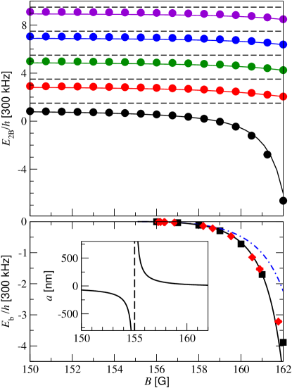
Figure 1: (Color online) Magnetic field dependence of the vibrational energy levels $E_{\mathrm{2B}}$ of a pair of ⁸⁵Rb atoms in a $\nu_{\mathrm{ho}}=300$ kHz trap (upper part) as compared to the binding energies of the highest excited vibrational state of the ⁸⁵Rb₂ dimer molecule in free space (lower part). The circles in the upper part indicate numerical solutions of the two-body Schrödinger equation for a microscopic interaction potential explicitly incorporating the exact scattering length as well as the exact asymptotic $-C_{6}/r^{6}$ interaction energy, while the solid curves indicate calculations using the separable potential approach of Appendix A. The diamonds in the lower part are experimental binding energies obtained from Ref. Claussen03 and the squares indicate results of full coupled channels calculations of S. Kokkelmans Kokkelmans_private04 . The solid curve indicates the dimer binding energies obtained from the separable potential approach, while the dashed dotted curve corresponds to their near resonant approximation of Eq. (5). The inset of the lower part of the figure shows the singularity of the scattering length at the magnetic field strength $B_{0}=155.041$ G Claussen03 .

The association of diatomic Feshbach molecules using magnetically tunable Feshbach resonances is closely related to the variation of the two-body energy spectrum under adiabatic changes of the magnetic field strength. Figure 1 shows such an energy spectrum versus the magnetic field strength $B$ for a pair of ⁸⁵Rb atoms in a tight spherically symmetric harmonic atom trap, whose high frequency of $\nu_{\mathrm{ho}}=300$ kHz may be realised in a microchip trap Westbrook or in an optical lattice Tiesinga00 . The details of the underlying calculations are explained in Appendix A. In Fig. 1 the binding energy of the Feshbach molecule in free space is shown for comparison. The spherical symmetry of the atom trap allows us to separate the centre of mass from the relative coordinates of the atoms BERW_FP28 ; Tiesinga00 ; Bolda02 , and only the relevant levels of the relative motion are depicted in Fig. 1. We have chosen the zero of energy, for each magnetic field strength, at the dissociation threshold of the entrance channel in free space. Following the adiabatic curves of the energies clearly reveals that a pair of ⁸⁵Rb atoms occupying the level closest to the threshold on the low field side of the zero energy resonance is transferred into the level of the Feshbach molecule when the magnetic field strength is varied adiabatically across the resonance. The energy of the trapped molecular level and the free space binding energy $E_{\mathrm{b}}$ approach one another as the magnetic field strength is increased. A similar statement applies to their wave functions. This reflects the physical concept of the adiabatic association of diatomic molecules in tight atom traps.

The two-body trap level closest to the dissociation threshold can, in principle, be prepared by loading a Bose-Einstein condensate adiabatically into an optical lattice. In the case of ⁸⁵Rb the negative background scattering length of $a_{\mathrm{bg}}=-443\ a_{0}$ prevents such a condensate from being stable on the low field side of the resonance. To produce ⁸⁵Rb₂ Feshbach molecules via an adiabatic sweep of the magnetic field strength, the Bose-Einstein condensate needs to be prepared on the high field side of the resonance before it is loaded into the lattice. The resonance then needs to be crossed as quickly as possible to reach its low field side and, at the same time, avoid a significant heating of the atomic cloud KGG04 . Such a sequence of magnetic field sweeps is described in Ref. Thompson04 in the context of the adiabatic association of ⁸⁵Rb₂ Feshbach molecules in a cold gas.

III Thomas and Efimov effects

In this section we discuss the Thomas and Efimov effects in the three-body energy spectra of interacting Bose atoms. We show that these phenomena occur when the binary scattering length is tuned by a magnetic field in the vicinity of a zero energy resonance. We then describe how the Efimov spectrum is modified in the presence of a trapping potential. Our results indicate that it is the lowest energetic Efimov trimer state that can be populated by adiabatic changes of the magnetic field strength.

III.1 Three-body energy levels in free space

Throughout this section, we consider three Bose atoms that interact pairwise through their binary potential. This assumption is justified for the description of weakly bound molecules, like the Efimov trimers in the present applications, whose inter-atomic separations very much exceed the van der Waals length. Tightly bound trimer molecules may be significantly influenced by genuinely three-body forces, which we shall neglect in the following. We assume furthermore that the binary potential supports at most a single bound state, the Feshbach molecule $|\psi_{\mathrm{b}}\rangle$. We thus neglect all tightly bound diatomic states, whose spatial extents are typically much smaller than the van der Waals length. In view of the large separation of the length scales between Efimov trimers and the Feshbach molecule on the one hand and the tightly bound dimer states on the other hand, we believe that this treatment provides an excellent approximation to the three-body states and their low energies we consider in this paper. We note, however, that any trimer state with an energy above the two-body ground level can, at least in principle, decay into a dimer bound state and a third free atom in accordance with energy conservation. As, in free space, the binding energies of three atoms are thus strictly limited, from above, by the two-body ground state energy, the trimer molecules under consideration are all in meta-stable states. Their associated lifetimes may depend sensitively on the details of the binary and three-body interactions.

Given that the binary interactions support just a single, arbitrarily weakly bound state, it has been predicted, in terms of a rigorous variational treatment by Thomas Thomas35 , that three particles can be comparatively tightly bound. The three-body ground state can persist even when the binary interactions are weakened in such a way that their only bound state ceases to exist. Such three-body bound states that exist in the absence of any bound two-body subsystem are usually referred to as Borromean states Borromean .

The Thomas scenario of Borromean states has been subsequently generalised by Efimov Efimov70 , in a striking way, predicting that the number of three-body bound states of identical Bosons increases beyond all limits when the energy of the only two-body bound state is tuned towards the dissociation threshold. Efimov’s effect is closely related to the spatial extent of the near resonant two-body bound state wave function, which is determined by the scattering length in accordance with Eq. (4). According to Efimov’s treatment, it is indeed the scattering length, rather than the range of the potential, that sets the scale of the range of the effective three-particle interactions at the low collision energies under consideration. When the two-body binding energy reaches the dissociation threshold these interactions therefore acquire a long range. In contrast to a short range binary potential, however, long range interactions can support infinitely many bound states Schwinger61 . All these Efimov states are spherically symmetric and their energies accumulate at the three-body dissociation threshold. Their number is predicted to follow, in the limit $|a|\to\infty$, the asymptotic relationship:

$$N_{\mathrm{Efimov}}\gtrsim\frac{1}{\pi}\log\left(p_{\mathrm{c}}\left|a\right|/\hbar\right).$$ (10)

Here $p_{\mathrm{c}}$ is a momentum parameter related to the range of the binary interactions. Efimov’s remarkable results have been subsequently confirmed by Amado and Noble Amado72 .

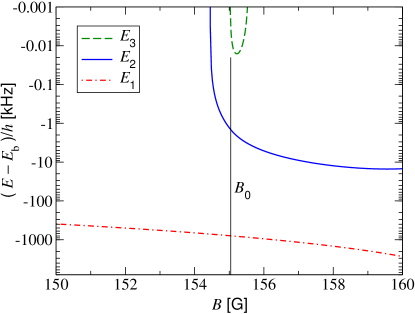
Figure 2: (Color online) Magnetic field dependence of the vibrational energy levels of ⁸⁵Rb₃ trimers relative to the binding energy $E_{\mathrm{b}}$ of the ⁸⁵Rb₂ Feshbach molecule (using $E_{\mathrm{b}}=0$ for $B<B_{0}$) in free space (cf. Fig. 1). The first Efimov states, whose energies are indicated by the solid and dashed curves, emerge at about $154.4$  G and $155$ G, respectively. The energies of the other Efimov states are not resolved even on the logarithmic energy scale. The second Efimov state (dashed curve) ceases to exist at about 155.5 G.

Efimov’s scenario can be realised, using the technique of Feshbach resonances, by magnetically tuning the binary scattering length of three Bose atoms in the vicinity of a zero energy resonance. Figure 2 shows the energy levels of three ⁸⁵Rb atoms in free space versus the magnetic field strength in the vicinity of the 155 G Feshbach resonance. The exact three-body binding energies have been determined using the momentum space Faddeev approach Gloeckle83 and the separable binary potential of Appendix A. According to Eq. (10), the number of Borromean Efimov states at negative binary scattering lengths increases beyond all limits when the pairwise attraction is strengthened in such a way that the two-body bound state emerges at the dissociation threshold. Two of their energies, i.e. the solid and dashed curves, are resolved on the logarithmic scale of Fig. 2. The dotted dashed curve is associated with the energy of the comparatively tightly bound Borromean state predicted by Thomas Thomas35 on the low field side of the zero energy resonance at $B_{0}=155.041$ G (vertical solid line).

It turns out that, as the bond of the dimer state is strengthened any further, the energies of the Efimov states successively cross the two-body binding energy and become unbound. Beyond the crossing point, the Efimov states can decay into a bound two-body subsystem, i.e. the Feshbach molecule, and a free particle, in accordance with energy conservation. This explains why the number of three-body bound states decreases as the attractive pairwise interactions are strengthened in the presence of a two-body bound state. In Fig. 2 we have chosen the zero of energy to be the three-body dissociation threshold, i.e. the binding energy $E_{\mathrm{b}}$ of the Feshbach molecule. The energy $E_{3}$ of the second Efimov state thus crosses the dimer binding energy at a magnetic field strength of 155.5 G.

Following the rigorous proof of Efimov’s effect by Amado and Noble Amado72 , the parameter $p_{\mathrm{c}}$ of Eq. (10) may be estimated, using the separable potential approach to the low energy spectrum of a pair of alkali atoms of Appendix A, to be:

$$p_{\mathrm{c}}\approx 2\hbar/(\pi\bar{a}).$$ (11)

In agreement with Thomas’ Thomas35 and Efimov’s Efimov70 original suggestions, Eq. (11) recovers the order of magnitude of $\hbar/r_{\mathrm{eff}}$, where $r_{\mathrm{eff}}=\frac{1}{3}[\Gamma(1/4)/\Gamma(3/4)]^{2}\bar{a}\approx 2.9\times\bar{a}$ is the effective range of the interaction between a pair of alkali atoms in the limit of large scattering lengths Flambaum99 ; Gao00 . Equation (11) thus confirms that, in contrast to the associated two-body problem, the low energy physics of three Bose atoms crucially depends on the range of the binary potential. In fact, in the hypothetical limit of a zero range potential not only the number of three-body bound states becomes infinite but also the three-body ground state energy diverges Thomas35 . This singular behaviour clearly reveals that the low energy three Boson problem is unsuited for a treatment in terms of pairwise contact interactions in the absence of energy cutoffs.

III.2 Adiabatic association of Efimov trimers in an atom trap

The spatial confinement of an atom trap restricts the bond length of the Feshbach molecule. This, in turn, implies that the energy levels of three trapped atoms, unlike those in free space, do not have any accumulation point even when the magnetic field strength is tuned across a singularity of the binary scattering length. Figure 3 reveals, however, that the energy spectrum of three ⁸⁵Rb atoms depends sensitively on the magnetic field strength, largely in analogy to the two-body spectrum of Fig. 1. The energy levels in Fig. 3 have been obtained from exact solutions of the Faddeev equations, in the presence of a spherically symmetric trapping potential, using the approach of Appendix B.

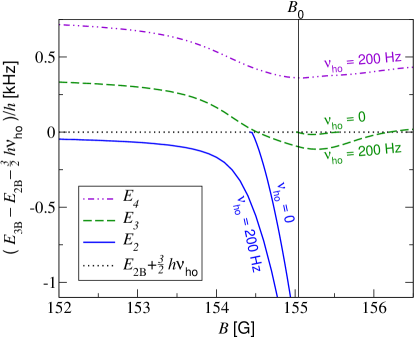
Figure 3: (Color online) Magnetic field dependence of the vibrational energy levels $E_{\mathrm{3B}}$ of three interacting ⁸⁵Rb atoms in a low frequency $\nu_{\mathrm{ho}}=200$ Hz trap as compared to the energies of the free space Efimov states of Fig. 2. The energies of the trapped atoms are shown relative to $E_{\mathrm{2B}}+\frac{3}{2}h\nu_{\mathrm{ho}}$, where we have chosen $E_{\mathrm{2B}}$ as the lowest energy of a pair of trapped ⁸⁵Rb atoms, i.e. the two-body level that correlates adiabatically, in the limit $\nu_{\mathrm{ho}}\to 0$, with the binding energy $E_{\mathrm{b}}$ of the Feshbach molecule of Fig. 1. In analogy, we have subtracted the dimer binding energy $E_{\mathrm{b}}$ from the Efimov trimer energies in free space for the purpose of comparison.

We have chosen the low frequency $\nu_{\mathrm{ho}}=200$ Hz of a typical magnetic atom trap in Fig. 3, which allows us to directly compare the energy levels of three ⁸⁵Rb atoms in the presence of the trap with those of the Efimov states in Fig. 2. This comparison shows that the trapped three-body energy level $E_{2}$ (solid curve), closest to the three-body dissociation threshold in free space (dotted horizontal line), correlates adiabatically, in the limit $\nu_{\mathrm{ho}}\to 0$, with the energy of the first Efimov state. A magnetic field pulse sequence similar to the one discussed in Subsection II.2 and in Ref. Thompson04 can, in principle, be used to populate the trapped three-body energy level associated with the solid curve in Fig. 3 on the low field side of $B_{0}$. An adiabatic upward sweep of the magnetic field strength across the three-body zero energy resonance of Fig. 2 at about 154.4 G then transfers the trapped state into the first Efimov state. The physical concept underlying the adiabatic association of Efimov trimers in atom traps is, therefore, completely analogous to the considerations on the production of diatomic Feshbach molecules in Subsection II.2.

IV Trimer molecules in an optical lattice

In this section we describe three interacting ⁸⁵Rb atoms in a tight micro-trap of an optical lattice site or in a microchip trap with a realistic oscillator frequency. Our results indicate that the spatial extent of the wave function of the first Efimov state can be tuned in such a way that it is smaller than realistic mean inter-atomic separations of dilute gases. We discuss, furthermore, how the periodicity of an optical lattice can, in principle, be used to detect the trimer molecules.

IV.1 Three-body energy levels and wave functions in tightly confining atom traps

The sites of an optical lattice, in general, confine the atoms much more tightly than usual magnetic traps for cold gases. Their harmonic frequencies differ by several orders of magnitude, from tens to hundreds of kHz in the case of a lattice Tiesinga00 or a microchip trap Long03 ; Westbrook as compared to about $100$ Hz for a conventional magnetic trap. During the course of our studies, we have calculated the energy levels of three ⁸⁵Rb atoms for a variety of trap frequencies extending from 200 Hz in Fig. 3 to 1 MHz. Our results indicate that, despite the pronounced differences in the spatial confinement, all spectra follow the same trends in their dependence on the magnetic field strength. The variation of the trap frequencies mainly affects the spacings between the energy levels. In fact, all our considerations with respect to the association of Efimov trimer molecules depend just on the possibility of trapping exactly three atoms rather than on the tightness of the spatial confinement.

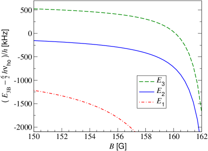
Figure 4: (Color online) Magnetic field dependence of the vibrational energy levels $E_{\mathrm{3B}}$ of three ⁸⁵Rb  atoms relative to the zero point energy $\frac{6}{2}h\nu_{\mathrm{ho}}$ of three hypothetically non-interacting atoms in a tightly confining $\nu_{\mathrm{ho}}=300$ kHz trap.

As a typical example of our results, Fig. 4 shows the energy levels of three ⁸⁵Rb atoms versus the magnetic field strength in a tightly confining atom trap with a frequency of $\nu_{\mathrm{ho}}=300$ kHz. We note that in Fig. 4 the energies are given relative to the zero point energy of three hypothetically non-interacting trapped atoms, while in Figs. 2 and 3 we have chosen the zero of energy at the three-body dissociation threshold in free space, i.e. at the binding energy $E_{\mathrm{b}}$ of the Feshbach molecule. The solid curve of $E_{2}$ in Fig. 4 thus correlates adiabatically, in the limit $\nu_{\mathrm{ho}}\to 0$, with the first Efimov state of Figs. 2 and 3. Figure 2 reveals that the trapped first Efimov state is transferred into a meta-stable trimer molecule, within a range of magnetic field strengths from 154.4 G to at least 160 G, when it is adiabatically released from the trap. The modulus of its binding energy is always slightly larger than $\left|E_{\mathrm{b}}\right|$. These predictions suggest that the adiabatic association of the first Efimov trimer state is, in principle, feasible and leads to reasonably strong bonds. We note that the production of the weakly bound ⁸⁵Rb₂ Feshbach molecules has been observed over a wide range of magnetic field strengths Thompson04 .

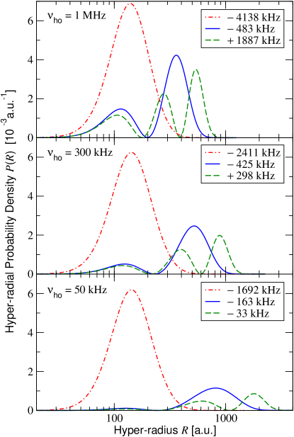
Figure 5: (Color online) Hyper-radial probability densities $P(R)$ of the lowest energetic vibrational states of three ⁸⁵Rb atoms at $B=158.1$ G for the trap frequencies $\nu_{\text{ho}}=1\,$MHz, $\nu_{\text{ho}}=300\,$kHz, and $\nu_{\text{ho}}=50\,$kHz. The legends show the associated energies of the interacting atoms relative to the zero point energy of three hypothetically non-interacting atoms, i.e. $E_{\mathrm{3B}}-\frac{6}{2}h\nu_{\mathrm{ho}}$. The hyper-radius is given on a logarithmic scale.

Weakly bound molecules, such as Efimov trimers, are characterised by a large spatial extent of their wave functions KGJB03 . In order to identify them as separate entities in a dilute gas, it is crucial for the size of the molecules to be much smaller than the mean spacing between their centres of mass. As discussed in Appendix B, even the isotropic wave functions of the Efimov trimers depend on three parameters and can therefore not be directly visualised. To give an impression of the spatial structure of their wave functions, Fig. 5 shows the hyper-radial probability densities $P(R)$ of the three lowest energetic ⁸⁵Rb trimer states, at a magnetic field strength of 158.1 G, for trap frequencies decreasing from $1\,$MHz down to $50\,$kHz. In analogy to the case of diatomic molecules, the number of zeros of $P(R)$ is related to the degree of excitation of the three-body energy state. The solid curves are associated with the first Efimov state, which can be produced through an adiabatic upward sweep of the magnetic field strength. The wave function of this state extends over a few hundreds of Bohr radii in the $1\,$MHz trap and completely decays at about $2000\,$a.u. in the case of the $50\,$kHz trap. The sizes of the trimer states produced are thus comparable to the single particle oscillator lengths ($a_{\mathrm{ho}}=[h/(m\nu_{\mathrm{ho}})]^{1/2}\approx 1000\,$a.u. for ⁸⁵Rb atoms in a 50 kHz trap). This indicates that the three atoms occupy a volume comparable to the size of the single atom oscillator ground state. Although these length scales very much exceed the spatial extent of even the most loosely bound observed diatomic ground state molecule (the helium dimer Grisenti00 ), realistic cold gases are usually sufficiently dilute that the wave functions of these Efimov trimers do not overlap each other once they are adiabatically released from the lattice (cf., e.g., Ref. Zwierlein03 for an estimate of the remarkably large bond lengths of ⁶Li₂ Feshbach molecules produced in a dilute gas).

IV.2 Detection of Efimov trimer molecules in an optical lattice

A variety of present day detection techniques for weakly bound Feshbach molecules in cold gases relies upon direct rf photo-dissociation spectroscopy Regal03 , atom loss and recovery measurements Strecker03 ; Thompson04 , or the spatial separation of the molecular cloud from the remnant atomic gas Herbig03 ; Duerr04 ; Xu03 . While all these techniques may be applicable, in one way or another, also to Efimov trimers, an optical lattice lends itself to a rather different approach to their detection; the mass spectrometry using the periodic light potential as a diffracting device. We shall focus in the following on the perspectives of the diffraction technique.

The crucial coherence properties of Bose-Einstein condensed atomic gases loaded into optical lattices have been studied in detail in Ref. Greiner02 . These experiments indicate that the possibility of diffraction depends on the weakness of the light potential. Contrary to this, the association of Efimov trimers requires high tunnelling barriers between the individual sites to protect the molecules against inelastic collisions. In accordance with Ref. Greiner02 , we expect that adiabatically releasing the lattice depth transfers the gas of the Efimov trimers produced from their insulating phase back into the super-fluid phase. Super-fluid gases in optical lattices, however, can be diffracted Greiner02 .

The spatial periodicity of the optical lattice implies that the momenta of the cold molecules, when released from the light potential, are determined by multiples of the reciprocal lattice vectors with a negligible spread under the conditions of super-fluidity. The associated quantised velocity transfers obtained from the lattice, and consequently also the diffraction angles, are therefore inversely proportional to the molecular mass. The principle of this mass selection technique has been demonstrated in several earlier experiments on the spatial separation of weakly bound helium dimers Grisenti00 ; Schoellkopf94 and trimers Schoellkopf94 as well as sodium dimers Chapman95 from molecular beams. The freely expanding ⁸⁵Rb Efimov trimers of the present applications may then be dissociated and imaged using the methods of Refs. Strecker03 ; Herbig03 ; Duerr04 ; Xu03 ; Thompson04 . The mass selection detection technique suggested in this paper is general and could be applied, for instance, also to diatomic Feshbach molecules.

We expect that the most serious constraint on the production and detection of Efimov trimers in optical lattices is their intrinsic meta-stability. In the special case of ⁸⁵Rb₃ molecules there are two mechanisms that can lead to their spontaneous dissociation: The first mechanism consists in the decay into a fast, tightly bound dimer molecule and a fast atom. The second decay scenario involves spin relaxation of a constituent of the trimer molecule in analogy to the studies of Refs. Thompson04 ; KTJ04 . While the present considerations do not allow us to estimate the molecular lifetimes associated with the first decay mechanism, it has been shown in Refs. Thompson04 ; KTJ04 that spin relaxation can be efficiently suppressed by increasing the spatial extent of the molecules. It can be ruled out completely for other atomic species, in which the individual atoms are prepared in their electronic ground state. We are, however, not aware of other well studied entrance channel dominated Feshbach resonances of identical Bose atoms besides ⁸⁵Rb.

V Conclusions

We have studied in this paper the association of weakly bound meta-stable trimer molecules from three free Bose atoms in the ground state of a tight micro-trap of an optical lattice site or of a microchip. Our approach takes advantage of a remarkable quantum phenomenon in three-body energy spectra, known as Efimov’s effect. Efimov’s effect occurs when the binary scattering length is tuned in the vicinity of a zero energy resonance and involves the emergence of infinitely many three-body molecular states. We have shown that this scenario can be realised by magnetically tuning the inter-atomic interactions using the technique of Feshbach resonances.

The association scheme for trimer molecules, suggested in this paper, involves an adiabatic sweep of the magnetic field strength across a three-body zero energy resonance and can be performed largely in analogy to the well known association of diatomic molecules via magnetically tunable Feshbach resonances. Our results indicate that the predicted binding energies and spatial extents of the Efimov trimer molecules produced are comparable in their magnitudes to the associated quantities of the diatomic Feshbach molecules. We have illustrated our general considerations for the example of ⁸⁵Rb  including a suggestion for a complete experimental scenario and a possible detection scheme.

Once the meta-stable trimer molecules are produced, the possibility of tuning the inter-atomic interactions using Feshbach resonances may, in principle, be exploited to study the Efimov property of the trimer state. Since, according to the predictions of this paper, it is the first Efimov state that gets associated in an adiabatic sweep of the magnetic field strength, the trimer molecules are expected to dissociate as the pairwise attraction between the atoms is strengthened. This, at first sight, counterintuitive scenario can be realised by tuning the magnetic field strength away from the zero energy resonance on the side of positive scattering lengths. Once the energy of the diatomic Feshbach molecule crosses the binding energy of the trimers, the Efimov states dissociate into the Feshbach molecule as well as a third free atom. In this way, the technique of Feshbach resonances could provide a unique opportunity to finally confirm this predicted Efimov70 but as yet unobserved fascinating quantum phenomenon in the energy spectrum of three Bose particles.

Appendix A Separable two-body interaction

In this appendix we provide a convenient effective binary interaction potential that well describes the relevant low energy vibrational levels of an atom pair, both in free space and under the strong spatial confinement of a tight micro-trap of an optical lattice site or of a microchip. We determine the parameters of the effective potential in terms of the $s$ wave binary scattering length $a$ and the van der Waals dispersion coefficient $C_{6}$, which characterises the interaction energy at asymptotically large inter-atomic distances.

A.1 Overview of the separable potential approach in free space

A.1.1 Hamiltonian

We first consider a pair of identical Bose atoms of mass $m$ at the positions $\bm{\mathrm{r}}_{1}$ and $\bm{\mathrm{r}}_{2}$, respectively, which interact via the microscopic potential $V$ in the absence of a confining atom trap. The associated free-space binary Hamiltonian is then given by the formula:

$$H_{\mathrm{free}}=H_{0}^{\mathrm{free}}+V.$$ (12)

Here the non-interacting Hamiltonian

$$H_{0}^{\mathrm{free}}=-\frac{\hbar^{2}}{2(2m)}\nabla_{\bm{\mathrm{R}}}^{2}-\frac{\hbar^{2}}{2(\frac{m}{2})}\nabla_{\bm{\mathrm{r}}}^{2}$$ (13)

accounts for the kinetic energy, where $\bm{\mathrm{R}}=\frac{1}{2}(\bm{\mathrm{r}}_{1}+\bm{\mathrm{r}}_{2})$ and $\bm{\mathrm{r}}=\bm{\mathrm{r}}_{1}-\bm{\mathrm{r}}_{2}$ denote the centre of mass and relative coordinates of the atom pair, respectively. We assume in the following that the centre of mass is at rest and focus only on the relative motion of the atom pair. The non-interacting Hamiltonian in free space then reduces to $\hat{H}_{0}^{\mathrm{free}}=-\hbar^{2}\nabla_{\bm{\mathrm{r}}}^{2}/m$.

A.1.2 Transition matrix

In our subsequent applications to three-body systems it will be convenient to represent all bound and free energy levels of the binary subsystems in terms of their transition matrix $\hat{T}(z)$ associated with the relative motion of the atoms, whose singularities as a function of the continuous variable $z$ determine the two-body energy spectrum. In general, the transition matrix associated with the interaction potential $V$ can be obtained from the Lippmann-Schwinger equation newton :

$$\hat{T}(z)=V+V\hat{G}_{0}^{\mathrm{free}}(z)\hat{T}(z).$$ (14)

Here $\hat{G}_{0}^{\mathrm{free}}(z)=(z-\hat{H}_{0}^{\mathrm{free}})^{-1}$ is the Green’s function of the relative motion of the atoms in the absence of inter-atomic interactions.

A.1.3 Low energy physical observables

The solution of the two-body Lippmann-Schwinger equation (14) for the microscopic inter-atomic potential $V(\bm{\mathrm{r}})$ is a demanding problem in its own right. The full binary interaction, however, describes a range of energies much larger than those accessible to cold collision physics. We shall therefore introduce a simpler effective potential which properly accounts just for the relevant low energy physical observables. Considerations GKGTJ_JPB37 beyond the scope of this paper show that all physical observables associated with cold binary collisions can be described by a single parameter, the $s$ wave scattering length $a$. The $T$ matrix determines the scattering length by its plane wave matrix elements in the limit of zero energy:

$$\langle\bm{\mathrm{p}}^{\prime}=0|\hat{T}(0)|\bm{\mathrm{p}}=0\rangle=\frac{1}{(2\pi\hbar)^{3}}\frac{4\pi\hbar^{2}}{m}a.$$ (15)

The very existence of the Thomas and Efimov effects clearly reveals that cold collisions of three Bose atoms are sensitive also to the spatial range of the interaction. At large distances $r$ the asymptotic form of the inter-atomic potential is given by $V(\bm{\mathrm{r}})\underset{r\to\infty}{\sim}-C_{6}/r^{6}$, where $C_{6}$ is the van der Waals dispersion coefficient. We shall thus determine the effective binary potential of alkali atoms in such a way that it provides a straightforward access to the full $T$ matrix and, at the same time, recovers the exact scattering length $a$ as well as those low energy physical observables that are sensitive also to $C_{6}$, such as, for instance, the the energies of the trapped atom pairs in Fig. 1. As shown in Ref. GF_PRA48 , the $C_{6}$ coefficient enters these measurable quantities in terms of the mean scattering length of Eq. (6). In our applications to energy spectra in the vicinity of a zero energy resonance the mean scattering length $\bar{a}$ determines the binding energy of the highest excited diatomic vibrational state (cf. Fig. 1) at positive scattering lengths $a$ by Eq. (7).

A.1.4 Solution of the Lippmann-Schwinger equation

To efficiently solve the two-body and three-body Schrödinger equations, it is convenient to choose a (non-local) separable potential of the general form (see, e.g., Ref. L_PR135 ; Sandhas72 ; Beliaev90 )

$$V_{\mathrm{sep}}=|g\rangle A\langle g|$$ (16)

as an effective replacement of the full microscopic binary interaction $V(\bm{\mathrm{r}})$. Here $|g\rangle$ is usually referred to as the form factor that sets the scale of the spatial range of the potential, while the amplitude $A$ determines the interaction strength. For convenience, we choose the form factor to be a Gaussian function in momentum space GKGTJ_JPB37 :

$$g(p)=\langle\bm{\mathrm{p}}|g\rangle=\left(\frac{\sigma^{2}}{\pi\hbar^{2}}\right)^{3/4}\exp\left(-\frac{p^{2}\sigma^{2}}{2\hbar^{2}}\right).$$ (17)

To adjust the amplitude $A$ and the range parameter $\sigma$ in such a way that $V_{\mathrm{sep}}$ recovers the scattering length $a$ as well as the mean scattering length $\bar{a}$ of the microscopic interaction potential $V(\bm{\mathrm{r}})$, we determine the full two-body energy spectrum associated with the separable potential via its transition matrix. We thus solve the Lippmann-Schwinger equation (14) formally, by iteration, in terms of its Born series:

$$\hat{T}_{\mathrm{sep}}(z)=\sum_{j=0}^{\infty}\left[V_{\mathrm{sep}}\hat{G}_{0}^{\mathrm{free}}(z)\right]^{j}V_{\mathrm{sep}}.$$ (18)

A simple derivation then shows that the $T$ matrix $\hat{T}_{\mathrm{sep}}(z)$ associated with $V_{\mathrm{sep}}$ is given by the formula:

$$\hat{T}_{\mathrm{sep}}(z)=|g\rangle\tau_{\mathrm{free}}(z)\langle g|.$$ (19)

Here the function $\tau_{\mathrm{free}}(z)$ can be determined from a geometric series to be:

$$\tau_{\mathrm{free}}(z)=\left[A^{-1}-\langle g|\hat{G}^{\mathrm{free}}_{0}(z)|g\rangle\right]^{-1}.$$ (20)

A.1.5 Adjustment of the separable potential

Evaluated at zero energy, $\tau_{\mathrm{free}}(z=0)$ is related to the $s$ wave binary scattering length $a$ through Eq. (15). Given the Gaussian form of $|g\rangle$ in Eq. (17), a spectral decomposition of the Green’s function $\hat{G}_{0}^{\mathrm{free}}(z)$ in terms of plane wave momentum states shows that its matrix element in Eq. (20) can be evaluated at zero energy to be $\langle g|\hat{G}^{\mathrm{free}}_{0}(0)|g\rangle=-2m\sigma^{2}/\hbar^{2}$. This leads to the relation

$$A=\frac{-\hbar^{2}/(2m\sigma^{2})}{1-\sqrt{\pi}\sigma/a},$$ (21)

which can be used to eliminate the amplitude $A$ in favour of the range parameter $\sigma$ and the scattering length $a$.

The single pole of $\tau_{\mathrm{free}}(z)$ at positive scattering lengths determines the energy $E_{\mathrm{b}}$ of the highest excited near resonant vibrational bound state (cf. Fig. 1). The adjustment of the energy $E_{\mathrm{b}}$ to Eq. (7) has been performed in Ref. GKGTJ_JPB37 and determines the remaining unknown range parameter to be:

$$\sigma=\sqrt{\pi}\bar{a}/2.$$ (22)

In our application to ⁸⁵Rb we use $\sigma=69.58$ a.u. which corresponds to $C_{6}=4703$ a.u. KKHV_PRL88 . The amplitude $A$ depends on the magnetic field strength $B$ via the scattering length $a$ in accordance with Eq. (21).

A.2 Energy levels of a trapped atom pair

A.2.1 Energy levels of the relative motion in the absence of an inter-atomic interaction

In the following applications we describe the micro-trap by a three dimensional spherically symmetric harmonic potential. The linear confining force then allows us to separate the centre of mass motion from the relative motion of a trapped atom pair BERW_FP28 ; Tiesinga00 ; Bolda02 . In the absence of an inter-atomic interaction the Hamiltonian of the relative motion is thus given by:

$$\hat{H}_{0}=-\frac{\hbar^{2}}{2\left(\frac{m}{2}\right)}\nabla_{\bm{\mathrm{r}}}^{2}+\frac{1}{2}\left(\frac{m}{2}\right)\omega_{\mathrm{ho}}^{2}\bm{\mathrm{r}}^{2}.$$ (23)

Here $\omega_{\mathrm{ho}}$ is the angular trap frequency. Throughout this appendix we choose energy states $|\varphi_{klm_{l}}\rangle$ of the harmonic oscillator with a definite orbital angular momentum, where $l$ is the angular momentum quantum number and $m_{l}$ is the orientation quantum number. The associated energies are given by $E_{kl}=\hbar\omega_{\mathrm{ho}}(2k+l+3/2)$, where $k=0,1,2,\ldots$ labels the vibrational excitation of the atom pair morsefeshbach . We denote the spherically symmetric vibrational energy states by $|\varphi_{k}\rangle=|\varphi_{k00}\rangle$ and their energies by $E_{k}=E_{k0}$. Their wave functions are given by

$$\varphi_{k}(r)=\sqrt{\frac{\beta^{3/2}}{2\pi}\frac{\Gamma(k+1)}{\Gamma(k+\frac{3}{2})}}\ e^{-\beta r^{2}/2}\ L_{k}^{(\frac{1}{2})}(\beta r^{2}),$$ (24)

where $L_{k}^{(\frac{1}{2})}$ is an associated Laguerre polynomial. The parameter $\beta=m\omega_{\mathrm{ho}}/(2\hbar)$ is related to the harmonic oscillator length $a_{\mathrm{ho}}$ for a single atom, i.e. the trap length, by $\beta=1/(2a_{\mathrm{ho}}^{2})$.

A.2.2 Separable potential approach in the presence of a trapping potential

The spherical symmetry of the trap allows us to determine the energy levels of the relative motion of a pair of interacting trapped atoms in complete analogy to their counterparts in free space BERW_FP28 ; Tiesinga00 ; Bolda02 . The associated Hamiltonian is then given by

$$\hat{H}=\hat{H}_{0}+V(\bm{\mathrm{r}}),$$ (25)

where $V(\bm{\mathrm{r}})$ is the spherically symmetric microscopic inter-atomic potential and $\hat{H}_{0}$ is the Hamiltonian of Eq. (23). In the following, we shall denote the energies associated with $\hat{H}$ by $E_{\mathrm{2B}}$.

Given that typically the trap length $a_{\mathrm{ho}}$ very much exceeds the van der Waals length $l_{\mathrm{vdW}}$, the full microscopic interaction can be replaced by the separable potential of Appendix A.1 to describe the limited range of energies involved in the adiabatic association of molecules. The associated $T$ matrix $\hat{T}_{\mathrm{sep}}(z)$ of the relative motion of a pair of trapped interacting atoms can then be determined in analogy to Appendix A.1. This yields:

$$\hat{T}_{\mathrm{sep}}(z)=|g\rangle\tau(z)\langle g|.$$ (26)

The function $\tau(z)$ can be obtained from Eq. (20) by replacing the Green’s function $\hat{G}_{0}^{\mathrm{free}}(z)$ in free space by its counterpart $\hat{G}_{0}(z)=(z-\hat{H}_{0})^{-1}$ in the presence of the trapping potential. This leads to the relation:

$$\tau(z)=\left[\left(\tau_{\mathrm{free}}(0)\right)^{-1}-4\left(\frac{m}{2}\right)\sigma^{2}/\hbar^{2}-\langle g|\hat{G}_{0}(z)|g\rangle\right]^{-1}.$$ (27)

The poles of $\tau(z)$ determine the energy levels of the Hamiltonian (25) in the separable potential approximation, i.e. the poles are located at the energies $z=E_{\mathrm{2B}}$.

We have evaluated the function $\tau(z)$ in terms of the oscillator states $|\varphi_{k}\rangle$ of Eq. (24) using the spectral decomposition of the Green’s function $\hat{G}_{0}(z)$. The matrix element relevant to Eq. (27) is given by:

$$\langle g|\hat{G}_{0}(z)|g\rangle=\sum_{k=0}^{\infty}\frac{\left|\langle\varphi_{k}|g\rangle\right|^{2}}{z-E_{k}}.$$ (28)

During the course of our studies, we have compared the separable potential approach to the two-body energy spectrum to predictions obtained with a microscopic potential $V(\bm{\mathrm{r}})$ for a variety of scattering lengths and trap frequencies. Figure 1 shows such a comparison for a rather tight $\nu_{\mathrm{ho}}=300$ kHz atom trap, which clearly reveals the applicability of the separable potential approach in the range of energies relevant to the adiabatic association of Efimov trimer molecules.

Appendix B Three-body energy levels and wave functions

In this appendix we derive the Faddeev equations that determine the exact energy levels of three interacting Bose atoms in the confining potential of a spherical trap. We then describe a practical method to exactly solve these equations in the separable potential approach.

B.1 Faddeev approach

B.1.1 Three-body Hamiltonian and Jacobi coordinates

Throughout this appendix, we assume that the atoms interact pairwise via the potential $V(\bm{\mathrm{r}})$. The complete Hamiltonian is then given by:

$$H=H_{0}+V(\bm{\mathrm{r}}_{23})+V(\bm{\mathrm{r}}_{31})+V(\bm{\mathrm{r}}_{12}).$$ (29)

Here the non-interacting Hamiltonian

$$H_{0}=\sum_{i=1}^{3}\left(-\frac{\hbar^{2}}{2m}\nabla_{\bm{\mathrm{r}}_{i}}^{2}+\frac{1}{2}m\omega_{\mathrm{ho}}^{2}\bm{\mathrm{r}}_{i}^{2}\right)$$ (30)

accounts for the kinetic energy and the harmonic trapping potential of each atom, while $V(\bm{\mathrm{r}}_{ij})$ describes the interaction between the atoms $i$ and $j$ ($i,j=1,2,3$) in dependence on their relative coordinates $\bm{\mathrm{r}}_{ij}=\bm{\mathrm{r}}_{i}-\bm{\mathrm{r}}_{j}$. In the following, we employ the Jacobi coordinates $\bm{\mathrm{R}}=(\bm{\mathrm{r}}_{1}+\bm{\mathrm{r}}_{2}+\bm{\mathrm{r}}_{3})/3$, $\bm{\mathrm{\rho}}=\bm{\mathrm{r}}_{1}-(\bm{\mathrm{r}}_{2}+\bm{\mathrm{r}}_{3})/2$ and $\bm{\mathrm{r}}=\bm{\mathrm{r}}_{2}-\bm{\mathrm{r}}_{3}$ of Fig. 6 to separate out the three-body centre of mass. In analogy to the case of a pair of trapped atoms, the harmonic force then allows us to divide the non-interacting three-body Hamiltonian of Eq. (30) into three harmonic oscillator contributions associated with the Jacobi coordinates. The binary potentials involve only the relative coordinates $\bm{\mathrm{\rho}}$ and $\bm{\mathrm{r}}$. The complete three-body Hamiltonian can thus be represented by:

$$H= -\frac{\hbar^{2}}{2(3m)}\nabla_{\bm{\mathrm{R}}}^{2}+\frac{1}{2}(3m)\omega_{\mathrm{ho}}^{2}\bm{\mathrm{R}}^{2}-\frac{\hbar^{2}}{2(\frac{2}{3}m)}\nabla_{\bm{\mathrm{\rho}}}^{2}$$

$$+\frac{1}{2}\left(\frac{2}{3}m\right)\omega_{\mathrm{ho}}^{2}\bm{\mathrm{\rho}}^{2}-\frac{\hbar^{2}}{2(\frac{m}{2})}\nabla_{\bm{\mathrm{r}}}^{2}+\frac{1}{2}\left(\frac{m}{2}\right)\omega_{\mathrm{ho}}^{2}\bm{\mathrm{r}}^{2}$$

$$+V\!\left(\bm{\mathrm{r}}\right)+V\!\left(\bm{\mathrm{\rho}}+\frac{1}{2}\bm{\mathrm{r}}\right)+V\!\left(\bm{\mathrm{\rho}}-\frac{1}{2}\bm{\mathrm{r}}\right).$$ (31)

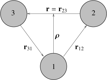
Figure 6: Jacobi coordinates of the relative motion of three atoms. The set of coordinates $\bm{\mathrm{\rho}}$ and $\bm{\mathrm{r}}$ is selected in such a way that it is suited to describe the hypothetical situation of an interacting pair of atoms $(2,3)$ with atom 1 playing the role of a spectator.

B.1.2 Faddeev equations for three trapped atoms

The Faddeev equations for the energy levels of three pairwise interacting atoms in the confining potential of a trap can be derived largely in analogy to their counterparts in free space F_JETP12 . To this end, we introduce the Green’s function

$$G_{0}(z)=(z-H_{0})^{-1}$$ (32)

associated with the non-interacting Hamiltonian of Eq. (30) and denote the binary potential associated with the atom pair $(i,j)$ by $V_{k}=V(\bm{\mathrm{r}}_{ij})$ for each of the three possible combinations of atomic indices

$$(ijk)=(1,2,3),(2,3,1),(3,1,2).$$

The stationary Schrödinger equation $H|\psi\rangle=E|\psi\rangle$ for a three-body energy state $|\psi\rangle$ can then be represented in terms of the matrix equation:

$$|\psi\rangle=G_{0}(E)\left(V_{1}+V_{2}+V_{3}\right)|\psi\rangle.$$ (33)

Introducing the Faddeev components

$$|\psi_{i}\rangle=G_{0}(E)V_{i}|\psi\rangle,$$ (34)

the three-body energy state is given by $|\psi\rangle=|\psi_{1}\rangle+|\psi_{2}\rangle+|\psi_{3}\rangle$. Inserting this Faddeev decomposition into Eq. (33) on the left hand side and rearranging the terms yields:

$$\left[1-G_{0}(E)V_{1}\right]|\psi_{1}\rangle=G_{0}(E)V_{1}\left(|\psi_{2}\rangle+|\psi_{3}\rangle\right).$$ (35)

Equation (35) can then be solved formally for $|\psi_{1}\rangle$ by multiplying both sides with $\left[1-G_{0}(E)V_{1}\right]^{-1}$ from the left. This leads to the Faddeev equation:

$$|\psi_{1}\rangle=\left[1-G_{0}(E)V_{1}\right]^{-1}G_{0}(E)V_{1}\left(|\psi_{2}\rangle+|\psi_{3}\rangle\right).$$ (36)

The kernel of Eq. (36) can then be expanded into the power series associated with the inverse matrix $\left[1-G_{0}(E)V_{1}\right]^{-1}$. This expansion yields:

$$\left[1-G_{0}(E)V_{1}\right]^{-1}G_{0}(E)V_{1}=G_{0}(E)\sum_{j=0}^{\infty}\left[V_{1}G_{0}(E)\right]^{j}V_{1}.$$ (37)

In analogy to Eq. (18), the sum on the right hand side of Eq. (37) can be identified as the Born series associated with the Lippmann-Schwinger equation:

$$T_{1}(z)=V_{1}+V_{1}G_{0}(z)T_{1}(z).$$ (38)

Representing Eq. (36) in terms of the $T$ matrix $T_{1}(E)$ for the interacting pair of atoms $(2,3)$ then recovers the Faddeev equation for $|\psi_{1}\rangle$ in its original form F_JETP12 :

$$|\psi_{1}\rangle=G_{0}(E)T_{1}(E)\left(|\psi_{2}\rangle+|\psi_{3}\rangle\right).$$ (39)

The Faddeev equations for $|\psi_{2}\rangle$ and $|\psi_{3}\rangle$ are obtained by cyclic permutations of the atomic indices. The resulting set of three coupled matrix equations for $|\psi_{1}\rangle$, $|\psi_{2}\rangle$ and $|\psi_{3}\rangle$ determines all energy levels of three interacting atoms in a trap. We note that the formal derivations leading to Eq. (39) do not refer to the specific nature of the confining potential. This is the reason for the general validity of the Faddeev approach in free space as well as in the presence of an atom trap.

B.1.3 Faddeev approach for three identical Bose atoms

In the special case of systems of three identical Bose atoms, such as ⁸⁵Rb₃, the three Faddeev components depend on each other through cyclic permutations of the atoms. These permutations can be represented by a unitary operator $\mathcal{U}$, i.e. $|\psi_{2}\rangle=\mathcal{U}|\psi_{1}\rangle$ and $|\psi_{3}\rangle=\mathcal{U}^{2}|\psi_{1}\rangle$, which transforms the three-body wave functions in accordance with the formula:

$$(\mathcal{U}\psi)(\bm{\mathrm{R}},\bm{\mathrm{\rho}},\bm{\mathrm{r}})=\psi(\bm{\mathrm{R}},\bm{\mathrm{\rho}}^{\prime},\bm{\mathrm{r}}^{\prime}).$$ (40)

Here the primed coordinates are determined by $\textstyle{{\bm{\mathrm{\rho^{\prime}}}}\choose{\bm{\mathrm{r^{\prime}}}}}=\mathcal{J}\textstyle{{\bm{\mathrm{\rho}}}\choose{\bm{\mathrm{r}}}}$, where

$$\mathcal{J}=\left(\begin{array}[]{rr}-\frac{1}{2}\mathbf{1}&\frac{3}{4}\mathbf{1}\\ -\mathbf{1}&-\frac{1}{2}\mathbf{1}\end{array}\right)$$ (41)

is a $6\times 6$ matrix satisfying $\mathcal{J}^{3}=1$. The first Faddeev component of Eq. (39) is thus determined by the single Faddeev equation:

$$|\psi_{1}\rangle=G_{0}(E)T_{1}(E)\left(\mathcal{U}+\mathcal{U}^{2}\right)|\psi_{1}\rangle.$$ (42)

B.1.4 Basis set expansion approach

In the following, we employ a basis set expansion approach to solve the Faddeev equation (42), which provides an extension of the momentum space Faddeev approach Gloeckle83 to systems of trapped atoms. Since, according to Eq. (31), the free Hamiltonian $H_{0}$ can be divided into a sum of three independent harmonic oscillators, we choose the basis of products

$$|\Phi_{KLM_{L}},\phi_{\kappa\lambda\mu_{\lambda}},\varphi_{klm_{l}}\rangle=|\Phi_{KLM_{L}}\rangle|\phi_{\kappa\lambda\mu_{\lambda}}\rangle|\varphi_{klm_{l}}\rangle$$ (43)

of the energy states of the individual oscillators with a definite angular momentum, i.e. $|\Phi_{KLM_{L}}\rangle$, $|\phi_{\kappa\lambda\mu_{\lambda}}\rangle$ and $|\varphi_{klm_{l}}\rangle$ are the oscillator energy states associated with the Jacobi coordinates $\bm{\mathrm{R}}$, $\bm{\mathrm{\rho}}$ and $\bm{\mathrm{r}}$, respectively.

The kernel of the Faddeev equation (42) is diagonal in the non-interacting energy states $|\Phi_{KLM_{L}}\rangle$. The component $|\psi_{1}\rangle$ can thus be chosen in such a way that it factorises into a centre of mass part and a relative part, i.e.

$$|\psi_{1}\rangle=|\Phi_{KLM_{L}}\rangle|\psi^{\mathrm{rel}}_{1}\rangle.$$ (44)

The relative part $|\psi^{\mathrm{rel}}_{1}\rangle$ then satisfies a reduced Faddeev equation at the shifted energy $E_{\mathrm{3B}}=E-E_{KL}$:

$$|\psi^{\mathrm{rel}}_{1}\rangle=G_{0}^{\mathrm{rel}}\left(E_{\mathrm{3B}}\right)T_{1}^{\mathrm{rel}}\left(E_{\mathrm{3B}}\right)\left[\mathcal{U}+\mathcal{U}^{2}\right]|\psi^{\mathrm{rel}}_{1}\rangle.$$ (45)

Here $G_{0}^{\mathrm{rel}}\left(E_{\mathrm{3B}}\right)$ and $T_{1}^{\mathrm{rel}}\left(E_{\mathrm{3B}}\right)$ can be interpreted in terms of a reduced non-interacting Green’s function and a reduced $T$ matrix, respectively, which depend only on the Jacobi coordinates $\bm{\mathrm{\rho}}$ and $\bm{\mathrm{r}}$ describing the relative motion of the three atoms.

In order to solve Eq. (45), the basis set expansion approach takes advantage of the convenient diagonal representation of the reduced non-interacting Green’s function in terms of the chosen basis states:

$$G_{0}^{\mathrm{rel}}(E_{\mathrm{3B}})=\sum_{\kappa,k\lambda,l=0}^{\infty}\sum_{\mu_{\lambda}=-\lambda}^{\lambda}\sum_{m_{l}=-l}^{l}\frac{|\phi_{\kappa\lambda\mu_{\lambda}},\varphi_{klm_{l}}\rangle\langle\phi_{\kappa\lambda\mu_{\lambda}},\varphi_{klm_{l}}|}{E_{\mathrm{3B}}-E_{\kappa\lambda}-E_{kl}}.$$ (46)

Since the reduced $T$ matrix $T_{1}^{\mathrm{rel}}\left(E_{\mathrm{3B}}\right)$ includes just the interaction between the pair of atoms $(2,3)$, it is related to the $T$ matrix $\hat{T}(z)$ of the relative motion of this atom pair by the formula:

$$\langle\phi_{\kappa\lambda\mu_{\lambda}},\varphi_{klm_{l}}|T_{1}^{\mathrm{rel}}(E_{\mathrm{3B}})|\phi_{\kappa^{\prime}\lambda^{\prime}\mu_{\lambda}^{\prime}},\varphi_{k^{\prime}l^{\prime}m_{l}^{\prime}}\rangle= \langle\varphi_{klm_{l}}|\hat{T}(z)|\varphi_{k^{\prime}l^{\prime}m_{l}^{\prime}}\rangle$$

$$\times\delta_{\kappa\kappa^{\prime}}\delta_{\lambda\lambda^{\prime}}\delta_{\mu_{\lambda}\mu^{\prime}_{\lambda}}.$$ (47)

Here $z=E_{\mathrm{3B}}-E_{\kappa\lambda}$ accounts for the energy of atom 1. The kernel of Eq. (42) is thus completely determined by the solution of the two-body Lippmann-Schwinger equation in the presence of the trapping potential.

The complete three-body energy state can be factorised in analogy to Eq. (44), i.e.

$$|\psi\rangle=|\Phi_{KLM_{L}}\rangle|\psi_{\mathrm{rel}}\rangle.$$ (48)

Given the solution of Eq. (45), the reduced Faddeev component $|\psi_{1}^{\mathrm{rel}}\rangle$ determines $|\psi_{\mathrm{rel}}\rangle$ by the relationship:

$$|\psi_{\mathrm{rel}}\rangle=\left(1+\mathcal{U}+\mathcal{U}^{2}\right)|\psi^{\mathrm{rel}}_{1}\rangle.$$ (49)

Equations (45), (46) and (47) set up our general approach to the energy spectrum of three interacting atoms in a trap, while Eqs. (48) and (49) yield the associated three-body energy states.

B.2 Solution of the Faddeev equations in the separable potential approach

B.2.1 Faddeev equations in the separable potential approach

We shall show in the following that the separable potential approach to the two-body $T$ matrix, in combination with the basis set expansion, provides a practical scheme to exactly solve the Faddeev equation (45) in the presence of a trapping potential. To this end, we apply Eqs. (47) and (26) to Eq. (45). This yields:

$$|\psi^{\mathrm{rel}}_{1}\rangle= G_{0}^{\mathrm{rel}}\left(E_{\mathrm{3B}}\right)\sum_{\kappa=0}^{\infty}\sum_{\lambda=0}^{\infty}\sum_{\mu_{\lambda}=-\lambda}^{\lambda}|\phi_{\kappa\lambda\mu_{\lambda}},g\rangle\tau\left(E_{\mathrm{3B}}-E_{\kappa\lambda}\right)$$

$$\times\langle\phi_{\kappa\lambda\mu_{\lambda}},g|\left[\mathcal{U}+\mathcal{U}^{2}\right]|\psi^{\mathrm{rel}}_{1}\rangle.$$ (50)

Equation (50) reveals that $|\psi^{\mathrm{rel}}_{1}\rangle$ is of the general form:

$$|\psi^{\mathrm{rel}}_{1}\rangle=G_{0}^{\mathrm{rel}}\left(E_{\mathrm{3B}}\right)|f,g\rangle.$$ (51)

As only the unknown amplitude $f_{\kappa\lambda\mu_{\lambda}}=\langle\phi_{\kappa\lambda\mu_{\lambda}}|f\rangle$ needs to be determined, the separable potential approach significantly simplifies the Faddeev equation (45) by reducing its dimensionality from six to three. We shall show in the following that due to the spherical symmetry of the form factor $|g\rangle$ the number of dimensions reduces even further to only one provided that the three-body energy levels under consideration have $s$ wave symmetry.

B.2.2 Basis set expansion

In accordance with the basis set expansion approach, we consider the projected amplitude $f_{\kappa\lambda\mu_{\lambda}}$. The ansatz of Eq. (51) for the solution of the Faddeev equation (50) then determines the amplitude $f_{\kappa\lambda\mu_{\lambda}}$ by the matrix equation:

$$f_{\kappa\lambda\mu_{\lambda}}=\tau\left(E_{\mathrm{3B}}-E_{\kappa\lambda}\right)\sum_{\kappa^{\prime}=0}^{\infty}\sum_{\lambda^{\prime}=0}^{\infty}\sum_{\mu_{\lambda}^{\prime}=-\lambda^{\prime}}^{\lambda^{\prime}}\mathcal{K}_{\kappa\lambda\mu_{\lambda},\kappa^{\prime}\lambda^{\prime}\mu_{\lambda}^{\prime}}\left(E_{\mathrm{3B}}\right)f_{\kappa^{\prime}\lambda^{\prime}\mu_{\lambda}^{\prime}}.$$ (52)

In accordance with Eq. (46), the reduced kernel matrix associated with this equation for $f_{\kappa\lambda\mu_{\lambda}}$ is given by the formula:

$$\mathcal{K}_{\kappa\lambda\mu_{\lambda},\kappa^{\prime}\lambda^{\prime}\mu_{\lambda}^{\prime}}\left(E_{\mathrm{3B}}\right)=\langle\phi_{\kappa\lambda\mu_{\lambda}},g|\left(\mathcal{U}+\mathcal{U}^{2}\right)G_{0}^{\mathrm{rel}}\left(E_{\mathrm{3B}}\right)|\phi_{\kappa^{\prime}\lambda^{\prime}\mu_{\lambda}^{\prime}},g\rangle.$$ (53)

The complete kernel also involves the function $\tau\left(E_{\mathrm{3B}}-E_{\kappa\lambda}\right)$ which we have discussed in detail in Appendix A.1. Inserting the spectral decomposition of the Green’s function of three non-interacting trapped atoms of Eq. (46) then determines the reduced kernel matrix to be:

$$\mathcal{K}_{\kappa\lambda\mu_{\lambda},\kappa^{\prime}\lambda^{\prime}\mu_{\lambda}^{\prime}}= \sum_{k,k^{\prime}=0}^{\infty}\sum_{l,l^{\prime}=0}^{\infty}\sum_{m_{l}=-l}^{l}\sum_{m_{l}^{\prime}=-l^{\prime}}^{l^{\prime}}\frac{\langle g|\varphi_{klm_{l}}\rangle\langle\varphi_{k^{\prime}l^{\prime}m_{l}^{\prime}}|g\rangle}{E_{\mathrm{3B}}-E_{\kappa^{\prime}\lambda^{\prime}}-E_{k^{\prime}l^{\prime}}}$$

$$\times\langle\phi_{\kappa\lambda\mu_{\lambda}},\varphi_{klm_{l}}|\left(\mathcal{U}+\mathcal{U}^{2}\right)|\phi_{\kappa^{\prime}\lambda^{\prime}\mu_{\lambda}^{\prime}},\varphi_{k^{\prime}l^{\prime}m_{l}^{\prime}}\rangle.$$ (54)

B.2.3 Symmetry considerations

The spherical symmetry of the form factor $|g\rangle$ of Eq. (17) implies that only the spherically symmetric basis states $|\varphi_{k}\rangle\equiv|\varphi_{k00}\rangle$ contribute to the summation in Eq. (54), i.e. $l=l^{\prime}=0$ and $m_{l}=m_{l}^{\prime}=0$. As, moreover, the total angular momentum operator $\bm{\mathrm{\mathcal{L}}}=\bm{\mathrm{\lambda}}+\bm{\mathrm{l}}$ associated with the three-body state $|\psi_{\mathrm{rel}}\rangle$ commutes with the permutation operator $\mathcal{U}$, the off-diagonal elements $\lambda\neq\lambda^{\prime}$ and $\mu\neq\mu_{\lambda}^{\prime}$ of the kernel vanish, i.e. the kernel does not couple solutions of different angular momenta $\bm{\mathrm{\lambda}}$. Furthermore, the Hamiltonian $H$ commutes with $\mathcal{U}$ which implies that the matrix element of $\left(\mathcal{U}+\mathcal{U}^{2}\right)$ in the reduced kernel matrix of Eq. (54) is non-zero only if

$$\kappa+k=\kappa^{\prime}+k^{\prime}.$$ (55)

This is a consequence of energy conservation.

We shall focus in the following on those energy states of three trapped interacting atoms that correlate adiabatically, in the limit of zero trap frequency, with the three-body $s$ wave Efimov states. We thus restrict the discussion to three-body states with zero total angular momentum $\mathcal{L}=0$. In this case all angular momentum quantum numbers are zero and may be omitted. This implies that the kernel matrix in Eq. (52) reduces to

$$\mathcal{K}_{\kappa\kappa^{\prime}}\left(E_{\mathrm{3B}}\right)=\sum_{k,k^{\prime}=0}^{\infty}\frac{g_{k}\langle\phi_{\kappa},\varphi_{k}|\left(\mathcal{U}+\mathcal{U}^{2}\right)|\phi_{\kappa^{\prime}},\varphi_{k^{\prime}}\rangle g_{k^{\prime}}}{E_{\mathrm{3B}}-E_{\kappa}-E_{k}},$$ (56)

and the amplitude $f_{\kappa}=\langle\phi_{\kappa}|f\rangle$ satisfies the matrix equation:

$$f_{\kappa}=\tau\left(E_{\mathrm{3B}}-E_{\kappa}\right)\sum_{\kappa^{\prime}=0}^{\infty}\mathcal{K}_{\kappa\kappa^{\prime}}\left(E_{\mathrm{3B}}\right)f_{\kappa^{\prime}}.$$ (57)

In accordance with the ansatz of Eq. (51), the first Faddeev component is then given in terms of the amplitude $f_{\kappa}$ and the form factor $g_{k}$ by the formula:

$$\langle\phi_{\kappa},\varphi_{k}|\psi_{1}^{\mathrm{rel}}\rangle=\frac{f_{\kappa}g_{k}}{E_{\mathrm{3B}}-E_{\kappa}-E_{k}}.$$ (58)

B.3 Determination of the kernel matrix

A main difficulty in the numerical determination of the amplitude $f_{\kappa}$ from Eq. (57) consists in calculating the reduced kernel matrix $\mathcal{K}_{\kappa\kappa^{\prime}}\left(E_{\mathrm{3B}}\right)$ for the variety of trap frequencies studied in this paper. While in tight atom traps ($\nu_{\mathrm{ho}}>100\,$kHz) the discrete nature of the energy levels is most significant, the opposite regime of low trap frequencies ($\nu_{\mathrm{ho}}<1\,$kHz) involves a large range of vibrational quantum numbers $\kappa$ leading to a continuum of modes in the limit $\nu_{\mathrm{ho}}\to 0$. To obtain a stable scheme for the determination of the reduced kernel matrix in the limits of both high and low trap frequencies, we have performed separate treatments of the regimes of low and high vibrational quantum numbers $\kappa$. Since these aspects of the studies of trapped systems of three interacting atoms differ significantly from the known techniques to solve the Faddeev equations in free space Gloeckle83 , we shall outline in detail the numerical procedure we have applied.

B.3.1 The kernel matrix at low vibrational excitations

In the limit of small $\kappa$ the determination of the reduced kernel matrix $\mathcal{K}_{\kappa\kappa^{\prime}}$ consists mainly of the calculation of the matrix elements

$$C_{\kappa k,\kappa^{\prime}k^{\prime}}=\langle\phi_{\kappa},\varphi_{k}|\left[\mathcal{U}+\mathcal{U}^{2}\right]|\phi_{\kappa^{\prime}},\varphi_{k^{\prime}}\rangle.$$ (59)

We perform this calculation in the configuration space representation. To this end, it is convenient to introduce the auxiliary function:

$$\psi_{k}(\beta;x)=\sqrt{\frac{\beta^{3/2}}{2\pi}\frac{\Gamma(k+1)}{\Gamma(k+\frac{3}{2})}}\ e^{-x/2}\ L_{k}^{(\frac{1}{2})}(x).$$ (60)

This function is related to the spherically symmetric harmonic oscillator states (cf. Appendix A.2) associated with the Jacobi coordinates $\bm{\mathrm{\rho}}$ and $\bm{\mathrm{r}}$ by the formulae

$$\phi_{\kappa}(\rho)= \psi_{\kappa}(\beta_{\rho};\beta_{\rho}\rho^{2}),$$ (61)

$$\varphi_{k}(r)= \psi_{k}(\beta_{r};\beta_{r}r^{2}),$$ (62)

respectively. Here the parameters $\beta_{\rho}=\frac{2}{3}m\omega_{\mathrm{ho}}/\hbar$ and $\beta_{r}=\frac{1}{2}m\omega_{\mathrm{ho}}/\hbar$ account for the different masses associated with the individual harmonic oscillator contributions to the three-body Hamiltonian (31). The matrix element involving the permutation operator can then be represented by:

$$C_{\kappa k,\kappa^{\prime}k^{\prime}}= \int d^{3}\rho\ d^{3}r\ \psi_{\kappa}(\beta_{\rho};\beta_{\rho}\rho^{2})\psi_{k}(\beta_{r};\beta_{r}r^{2})$$

$$\times\left[\psi_{\kappa^{\prime}}(\beta_{\rho};\beta_{\rho}\rho^{\prime 2})\psi_{k^{\prime}}(\beta_{r};\beta_{r}r^{\prime 2})\right.$$

$$+\left.\psi_{\kappa^{\prime}}(\beta_{\rho};\beta_{\rho}\rho^{\prime\prime 2})\psi_{k^{\prime}}(\beta_{r};\beta_{r}r^{\prime\prime 2})\right].$$ (63)

Here the permutation operators $\mathcal{U}$ and $\mathcal{U}^{2}$ transform the coordinates $\bm{\mathrm{\rho}}$ and $\bm{\mathrm{r}}$ into primed and double primed coordinates $\textstyle{{\bm{\mathrm{\rho}}^{\prime}}\choose{\bm{\mathrm{r}}^{\prime}}}=\mathcal{J}\textstyle{{\bm{\mathrm{\rho}}}\choose{\bm{\mathrm{r}}}}$ and $\textstyle{{\bm{\mathrm{\rho}}^{\prime\prime}}\choose{\bm{\mathrm{r}}^{\prime\prime}}}=\mathcal{J}^{2}\textstyle{{\bm{\mathrm{\rho}}}\choose{\bm{\mathrm{r}}}}$, respectively, in accordance with the transformation matrix $\mathcal{J}$ of Eq. (41). The transformation with $\mathcal{J}$ yields:

$$\beta_{\rho}\rho^{\prime 2}= \frac{1}{4}\beta_{\rho}\rho^{2}+\frac{3}{4}\beta_{r}r^{2}-\sqrt{\frac{3}{4}\beta_{\rho}\beta_{r}}\ \bm{\mathrm{\rho}}\cdot\bm{\mathrm{r}},$$ (64)

$$\beta_{r}r^{\prime 2}= \frac{3}{4}\beta_{\rho}\rho^{2}+\frac{1}{4}\beta_{r}r^{2}+\sqrt{\frac{3}{4}\beta_{\rho}\beta_{r}}\ \bm{\mathrm{\rho}}\cdot\bm{\mathrm{r}}.$$ (65)

This implies the relationship:

$$\beta_{\rho}\rho^{\prime 2}+\beta_{r}r^{\prime 2}=\beta_{\rho}\rho^{2}+\beta_{r}r^{2}.$$ (66)

Similar relations hold for the double primed coordinates with the reversed signs in front of the square roots. The integrand on the right hand side of Eq. (63), therefore, depends only on the variables $\rho$ and $r$ in addition to the variable $x=\bm{\mathrm{\rho}}\cdot\bm{\mathrm{r}}/(\rho r)$, which involves the angle between the coordinates $\bm{\mathrm{\rho}}$ and $\bm{\mathrm{r}}$. The integration over the remaining three variables is readily performed and leads to the formula:

$$C_{\kappa k,\kappa^{\prime}k^{\prime}}= 4(2\pi)^{2}\int_{0}^{\infty}\rho^{2}d\rho\ \int_{0}^{\infty}r^{2}dr\ \psi_{\kappa}(\beta_{\rho};\beta_{\rho}\rho^{2})\psi_{k}(\beta_{r};\beta_{r}r^{2})$$

$$\times\int_{-1}^{1}dx\ \psi_{\kappa^{\prime}}\left(\beta_{\rho};\frac{1}{4}\beta_{\rho}\rho^{2}+\frac{3}{4}\beta_{r}r^{2}-\sqrt{\frac{3}{4}\beta_{\rho}\beta_{r}}\rho rx\right)$$

$$\times\psi_{k^{\prime}}\left(\beta_{r};\frac{3}{4}\beta_{\rho}\rho^{2}+\frac{1}{4}\beta_{r}r^{2}+\sqrt{\frac{3}{4}\beta_{\rho}\beta_{r}}\rho rx\right).$$ (67)

This formula can be further evaluated by changing the variables to $u=\beta_{\rho}\rho^{2}$ and $v=\beta_{r}r^{2}$ and using the explicit form of the harmonic oscillator wave functions of Eq. (60). This evaluation yields:

$$C_{\kappa k,\kappa^{\prime}k^{\prime}}=\sqrt{\frac{\Gamma(\kappa+1)}{\Gamma(\kappa+\frac{3}{2})}\frac{\Gamma(k+1)}{\Gamma(k+\frac{3}{2})}\frac{\Gamma(\kappa^{\prime}+1)}{\Gamma(\kappa^{\prime}+\frac{3}{2})}\frac{\Gamma(k^{\prime}+1)}{\Gamma(k^{\prime}+\frac{3}{2})}}\ I_{\kappa k,\kappa^{\prime}k^{\prime}}.$$ (68)

The coefficients $I_{\kappa k,\kappa^{\prime}k^{\prime}}$ that involve the associated Laguerre polynomials read:

$$I_{\kappa k,\kappa^{\prime}k^{\prime}}= \int_{0}^{\infty}du\ u^{\frac{1}{2}}e^{-u}L_{\kappa}^{(\frac{1}{2})}(u)\int_{0}^{\infty}dv\ v^{\frac{1}{2}}e^{-v}L_{k}^{(\frac{1}{2})}(v)$$

$$\times\int_{-1}^{1}dx\ P_{\kappa^{\prime}k^{\prime}}(u,v,x).$$ (69)

Here the function

$$P_{\kappa^{\prime}k^{\prime}}(u,v,x)= L_{\kappa^{\prime}}^{(\frac{1}{2})}\left(\frac{1}{4}u+\frac{3}{4}v-\sqrt{\frac{3}{4}uv}x\right)$$

$$\times L_{k^{\prime}}^{(\frac{1}{2})}\left(\frac{3}{4}u+\frac{1}{4}v+\sqrt{\frac{3}{4}uv}x\right)$$ (70)

is a polynomial of degree $\kappa^{\prime}+k^{\prime}$ in the variable $x$. These derivations reveal that the matrix element in Eq. (68) is independent not only of the inter-atomic interaction potential but also of the frequency of the atom trap. The trap frequency enters Eq. (57) through the projections of the form factor onto the basis states and through the energy denominator.

To further evaluate Eq. (69), we represent the function $P_{\kappa^{\prime}k^{\prime}}(u,v,x)$ by the sum:

$$P_{\kappa^{\prime}k^{\prime}}(u,v,x)=\sum_{\gamma=0}^{\kappa^{\prime}+k^{\prime}}P_{\kappa^{\prime}k^{\prime}}^{\gamma}(u,v)x^{\gamma}.$$ (71)

Here the coefficients $P_{\kappa^{\prime}k^{\prime}}^{\gamma}(u,v)$ depend on the variables $u$ and $v$. Equation (71) then allows us to perform the integration over the variable $x$ in Eq. (69). Only the even powers $x^{\gamma}$ of the variable $x$ contribute to this integral, while all terms involving the odd powers vanish. When $\gamma$ is even, however, it turns out that the coefficients $P_{\kappa^{\prime}k^{\prime}}^{\gamma}(u,v)$ themselves are bivariate polynomials in the variables $u$ and $v$ and can also be expanded in powers of $u$ and $v$ with expansion coefficients $P_{\kappa^{\prime}k^{\prime}}^{\gamma\tau t}$. This expansion thus yields:

$$P_{\kappa^{\prime}k^{\prime}}^{\gamma}(u,v)=\sum_{\tau=0}^{\kappa^{\prime}+k^{\prime}}\sum_{t=0}^{\kappa^{\prime}+k^{\prime}-\tau}P_{\kappa^{\prime}k^{\prime}}^{\gamma\tau t}u^{\tau}v^{t}.$$ (72)

The representation of the expansion coefficients $P_{\kappa^{\prime}k^{\prime}}^{\gamma}(u,v)$ in Eq. (72) in terms of a polynomial allows us to take advantage of the general formula

$$\int_{0}^{\infty}du\ u^{\frac{1}{2}}e^{-u}L_{\kappa}^{(\frac{1}{2})}(u)u^{\tau}=\left\{\begin{array}[]{c@{\,:\,}r}0&0\leq\tau<\kappa\\ (-1)^{\kappa}\Gamma(\tau+\frac{3}{2})\binom{\tau}{\kappa}&\qquad\kappa\leq\tau\end{array}\right.$$ (75)

to perform the remaining integrations in Eq. (69) over the variables $u$ and $v$. Here $\binom{\tau}{\kappa}$ is a combinatorial. Equation (75) thus determines the coefficients $I_{\kappa k,\kappa^{\prime}k^{\prime}}$ of Eq. (69) to be:

$$I_{\kappa k,\kappa^{\prime}k^{\prime}}= (-1)^{\kappa^{\prime}+k^{\prime}}\sum^{\kappa^{\prime}+k^{\prime}}_{{\gamma=0}\atop{(\gamma\ \mathrm{even})}}\!\!\frac{2}{\gamma+1}\sum_{\tau=\kappa}^{\kappa^{\prime}+k^{\prime}}\Gamma\left(\tau+\frac{3}{2}\right)\binom{\tau}{\kappa}$$

$$\times\sum_{t=k}^{\kappa^{\prime}+k^{\prime}-\tau}\Gamma\left(t+\frac{3}{2}\right)\binom{t}{k}P_{\kappa^{\prime}k^{\prime}}^{\gamma\tau t}.$$ (76)

The limits of the different sums in Eq. (76) lead to a further simplification in the determination of $I_{\kappa k,\kappa^{\prime}k^{\prime}}$ as follows: The summation over the index $t$ is limited by the condition $\kappa^{\prime}+k^{\prime}-\tau\geq k$, which, together with the condition $\tau\geq\kappa$ for the index $\tau$, implies the inequality $\kappa^{\prime}+k^{\prime}\geq\kappa+k$. Similar considerations show that also the inequality $\kappa^{\prime}+k^{\prime}\leq\kappa+k$ is fulfilled, which, in summary, leads to the restriction $\kappa+k=\kappa^{\prime}+k^{\prime}$. These explicit derivations simply recover Eq. (55), which we have obtained independently from general symmetry considerations. Consequently, the summations over $\tau$ and $t$ in Eq. (76) reduce to a single term determined by $\tau=\kappa$ and $t=k$. This gives the coefficient $I_{\kappa k,\kappa^{\prime}k^{\prime}}$ to be:

$$I_{\kappa k,\kappa^{\prime}k^{\prime}}=(-1)^{\kappa+k}\ \Gamma\left(\kappa+\frac{3}{2}\right)\Gamma\left(k+\frac{3}{2}\right)\sum^{\kappa+k}_{{\gamma=0}\atop{(\gamma\ \mathrm{even})}}\!\!\frac{2}{\gamma+1}P_{\kappa^{\prime}k^{\prime}}^{\gamma\kappa k}.$$ (77)

The remaining, as yet, undetermined expansion coefficients $P_{\kappa^{\prime}k^{\prime}}^{\gamma\kappa k}$ of Eq. (72) can be obtained from the explicit form of the associated Laguerre polynomials, i.e. $L_{\kappa}^{(\frac{1}{2})}(x)=\sum_{\nu=0}^{\kappa}c_{\kappa\nu}x^{\nu}$, and their expansion coefficients:

$$c_{\kappa\nu}=(-1)^{\nu}\frac{1}{\nu!}\binom{\kappa+\frac{1}{2}}{\kappa-\nu}.$$ (78)

To this end, we consider the function $P_{\kappa^{\prime}k^{\prime}}^{\gamma}(u,v)$ of Eq. (71), whose explicit form can be determined from Eq. (70) to be:

$$P_{\kappa^{\prime}k^{\prime}}^{\gamma}(u,v)= \left(\frac{3}{4}\right)^{\frac{\gamma}{2}}(uv)^{\frac{\gamma}{2}}\sum_{\nu=0}^{\kappa^{\prime}}c_{\kappa^{\prime}\nu}\sum_{n=0}^{k^{\prime}}c_{k^{\prime}n}\sum_{\alpha=\max(0,\gamma-n)}^{\min(\nu,\gamma)}(-1)^{\alpha}\binom{\nu}{\alpha}$$

$$\times\binom{n}{\gamma-\alpha}\left(\frac{1}{4}u+\frac{3}{4}v\right)^{\nu-\alpha}\left(\frac{3}{4}u+\frac{1}{4}v\right)^{n+\alpha-\gamma}.$$ (79)

Equations (72) and (79) then give the remaining expansion coefficients $P_{\kappa^{\prime}k^{\prime}}^{\gamma\kappa k}$ to be:

$$P_{\kappa^{\prime}k^{\prime}}^{\gamma\kappa k}= 4^{\frac{\gamma}{2}-\kappa-k}c_{\kappa^{\prime}\kappa^{\prime}}c_{k^{\prime}k^{\prime}}\!\!\!\sum_{\alpha=\max(0,\gamma-k^{\prime})}^{\min(\kappa^{\prime},\gamma)}\!\!\!\!\!\!(-1)^{\alpha}\binom{\kappa^{\prime}}{\alpha}\binom{k^{\prime}}{\gamma-\alpha}$$

$$\times\sum_{\eta=\max(0,\kappa^{\prime}-\kappa-\alpha+\frac{\gamma}{2})}^{\min(\kappa^{\prime}-\alpha,k-\frac{\gamma}{2})}\binom{\kappa^{\prime}-\alpha}{\eta}\binom{k^{\prime}+\alpha-\gamma}{k-\frac{\gamma}{2}-\eta}\ 3^{\kappa-\kappa^{\prime}+\alpha+2\eta}.$$ (80)

In order to summarise our results in a concise form, we introduce the coefficients

$$\tilde{P}_{\kappa^{\prime}k^{\prime}}^{\gamma\kappa k}=\frac{P_{\kappa^{\prime}k^{\prime}}^{\gamma\kappa k}}{c_{\kappa^{\prime}\kappa^{\prime}}c_{k^{\prime}k^{\prime}}}=(-1)^{\kappa+k}\ \Gamma(\kappa^{\prime}+1)\Gamma(k^{\prime}+1)P_{\kappa^{\prime}k^{\prime}}^{\gamma\kappa k},$$ (81)

which are obtained simply by dividing $P_{\kappa^{\prime}k^{\prime}}^{\gamma\kappa k}$ of Eq. (80) by the expansion coefficients $c_{\kappa^{\prime}\kappa^{\prime}}=(-1)^{\kappa^{\prime}}/\Gamma(\kappa^{\prime}+1)$ and $c_{k^{\prime}k^{\prime}}=(-1)^{k^{\prime}}/\Gamma(k^{\prime}+1)$ of the associated Laguerre polynomials. An analysis of its summation limits shows that the sum over $\eta$ in Eq. (80) vanishes unless the conditions $\gamma\leq 2\kappa$ and $\gamma\leq 2k$ are fulfilled. In accordance with Eq. (77), we thus obtain:

$$I_{\kappa k,\kappa^{\prime}k^{\prime}}=\frac{\Gamma\left(\kappa+\frac{3}{2}\right)\Gamma\left(k+\frac{3}{2}\right)}{\Gamma\left(\kappa^{\prime}+1\right)\Gamma\left(k^{\prime}+1\right)}\sum^{\min(\kappa+k,2\kappa,2k)}_{{\gamma=0}\atop{(\gamma\ \mathrm{even})}}\frac{2}{\gamma+1}\tilde{P}_{\kappa^{\prime}k^{\prime}}^{\gamma\kappa k}.$$ (82)

The complete matrix element of Eq. (63) is then determined by the formula:

$$C_{\kappa k,\kappa^{\prime}k^{\prime}}= \sqrt{\frac{\Gamma(\kappa+1)}{\Gamma(\kappa^{\prime}+1)}\frac{\Gamma(\kappa+\frac{3}{2})}{\Gamma(\kappa^{\prime}+\frac{3}{2})}\frac{\Gamma(k+1)}{\Gamma(k^{\prime}+1)}\frac{\Gamma(k+\frac{3}{2})}{\Gamma(k^{\prime}+\frac{3}{2})}}$$

$$\times\sum^{\min(\kappa+k,2\kappa,2k)}_{{\gamma=0}\atop{(\gamma\ \mathrm{even})}}\!\!\frac{2}{\gamma+1}\tilde{P}_{\kappa^{\prime}k^{\prime}}^{\gamma\kappa k}.$$ (83)

Since the triple summation over $\alpha$, $\eta$ and $\gamma$ in Eqs. (80) and (83) contains only integer numbers, the calculation of the matrix element $C_{\kappa k,\kappa^{\prime}k^{\prime}}$ is, in principle, straightforward. As these numbers can, however, be very large in magnitude and have alternating signs, we have employed a computer algebra system to carry out the sum in multi-precision integer arithmetic. This proved practical for the indices $0\leq\kappa,\kappa^{\prime}\lesssim 40$.

B.3.2 The kernel matrix in the limit of high vibrational excitations

The numerical determination of the matrix element $C_{\kappa k,\kappa^{\prime}k^{\prime}}$ using Eq. (83) becomes impractical in the limit of large indices $\kappa$ and $\kappa^{\prime}$. We shall, therefore, provide a scheme to directly determine the reduced kernel matrix for these higher vibrational quantum numbers in terms of its asymptotic form in the continuum limit. Starting from Eq. (53) evaluated at zero angular momenta $\lambda=0$ and $\lambda^{\prime}=0$, the exact reduced kernel matrix is given by the formula:

$$\mathcal{K}_{\kappa\kappa^{\prime}}\left(E_{\mathrm{3B}}\right)= \langle\phi_{\kappa},g|\left(\mathcal{U}+\mathcal{U}^{2}\right)G_{0}^{\mathrm{rel}}\left(E_{\mathrm{3B}}\right)|\phi_{\kappa^{\prime}},g\rangle$$

$$= \sum_{k=0}^{\infty}\frac{\langle\phi_{\kappa},g|\left(\mathcal{U}+\mathcal{U}^{2}\right)|\phi_{\kappa^{\prime}},\phi_{k}\rangle\langle\phi_{k}|g\rangle}{E_{\mathrm{3B}}-E_{\kappa^{\prime}}-E_{k}}.$$ (84)

It turns out that, due to the permutation operators, the right hand side of Eq. (84) depends just on the oscillator wave functions $\phi_{\kappa}(\rho)$, $\phi_{\kappa^{\prime}}(\rho)$ and $\phi_{k}(r)$ in a limited range of radii $\rho$ and $r$ set by the width of the form factor $g(r)$. The typical length scale associated with the width of $g(r)$ is set by the range parameter $\sigma$ of Eq. (22) and is thus determined by the van der Waals length $l_{\mathrm{vdW}}$. As the van der Waals length is typically much smaller than the harmonic oscillator length $a_{\mathrm{ho}}=\sqrt{\hbar/(m\omega_{\mathrm{ho}})}$, the trapping potential is flat within the relevant range of radii $\rho,r\lesssim\sigma$ and the potential energy is much smaller than the mean kinetic energy of the highly excited oscillator states. We can, therefore, replace in Eq. (84) the Green’s function $G_{0}^{\mathrm{rel}}\left(E_{\mathrm{3B}}\right)$ of the trapping potential by its counterpart $G_{0}^{\mathrm{free}}\left(E_{\mathrm{3B}}\right)$ in free space and perform the continuum limit of the oscillator states $|\phi_{\kappa}\rangle$ and $|\phi_{\kappa^{\prime}}\rangle$.

Given that the radius $\rho$ is limited by the condition $\rho\lesssim\sigma$, in the continuum limit the harmonic oscillator energy wave functions $\phi_{\kappa\lambda\mu_{\lambda}}(\bm{\mathrm{\rho}})$ approach, up to a normalisation constant, the partial waves $|q\lambda\mu_{\lambda}\rangle$, i.e. the improper energy states of the free space Hamiltonian

$$H_{\rho}=-\frac{\hbar^{2}}{2(\frac{2}{3}m)}\nabla_{\bm{\mathrm{\rho}}}^{2}$$ (85)

with a definite angular momentum.

These partial waves thus satisfy the Schrödinger equation $H_{\rho}|q\lambda\mu_{\lambda}\rangle=E_{q}|q\lambda\mu_{\lambda}\rangle$, associated with the kinetic energy $E_{q}=q^{2}/[2(\frac{2}{3}m)]$, and are related to the plane waves $|\bm{\mathrm{q}}^{\prime}\rangle$ by

$$\langle\bm{\mathrm{q}}^{\prime}|q\lambda\mu_{\lambda}\rangle=(-i)^{\lambda}\ q^{-2}\delta(q-q^{\prime})Y_{\lambda}^{\mu_{\lambda}}(\bm{\mathrm{q}}^{\prime}/q^{\prime}),$$ (86)

where $Y_{\lambda}^{\mu_{\lambda}}$ is a spherical harmonic.

To determine the asymptotic form of the reduced kernel matrix in the limit of high vibrational excitations, we insert into Eq. (84) two complete sets of improper states $|q\lambda\mu_{\lambda}\rangle$ and $|q^{\prime}\lambda^{\prime}\mu_{\lambda}^{\prime}\rangle$. This yields:

$$\mathcal{K}_{\kappa\kappa^{\prime}}\left(E_{\mathrm{3B}}\right)\underset{\kappa,\kappa^{\prime}\to\infty}{\sim} \int_{0}^{\infty}\!\!\!dq\,q^{2}\langle\phi_{\kappa}|q00\rangle\!\int_{0}^{\infty}\!\!\!dq^{\prime}\,q^{\prime 2}\langle q^{\prime}00|\phi_{\kappa^{\prime}}\rangle$$

$$\times\langle q00,g|\left(\mathcal{U}+\mathcal{U}^{2}\right)G_{0}^{\mathrm{free}}\left(E_{\mathrm{3B}}\right)|q^{\prime}00,g\rangle.$$ (87)

A simple calculation then shows that for high vibrational quantum numbers $\kappa$ the function $q^{2}\langle\phi_{\kappa}|q00\rangle$ is sharply peaked about the central momentum $\bar{q}$ at the matched energies $E_{\kappa}=E_{q}$. This implies:

$$\bar{q}=\sqrt{\frac{4}{3}m\hbar\omega_{\mathrm{ho}}\left(2\kappa+\frac{3}{2}\right)}.$$ (88)

A similar relation holds for the central momentum $\bar{q}^{\prime}$ associated with the function $q^{\prime 2}\langle q^{\prime}00|\phi_{\kappa^{\prime}}\rangle$. We may, therefore, evaluate the slowly varying matrix element $\langle q00,g|\left(\mathcal{U}+\mathcal{U}^{2}\right)G_{0}^{\mathrm{free}}\left(E_{\mathrm{3B}}\right)|q^{\prime}00,g\rangle$ in Eq. (87) at $q=\bar{q}$ and $q^{\prime}=\bar{q}^{\prime}$. The remaining integration over $q$ then yields

$$\int_{0}^{\infty}\!\!\!dq\,q^{2}\langle\phi_{\kappa}|q00\rangle=2\left(\frac{2m\hbar\omega_{\mathrm{ho}}}{3}\right)^{3/4}\sqrt{\frac{\Gamma(\kappa+\frac{3}{2})}{\Gamma(\kappa+1)}},$$ (89)

and the integration over $q^{\prime}$ can be performed in an analogous way. Using the spectral decomposition of the free space Green’s function in terms of plane wave momentum states and the explicit Gaussian expression for the form factor in Eq. (17), the remaining matrix element $\langle\bar{q}00,g|\left(\mathcal{U}+\mathcal{U}^{2}\right)G_{0}^{\mathrm{free}}\left(E_{\mathrm{3B}}\right)|\bar{q}^{\prime}00,g\rangle$ can be determined analytically. In the limit of high vibrational excitations $\kappa$ and $\kappa^{\prime}$ the reduced kernel matrix is then given by the formula:

$$\mathcal{K}_{\kappa\kappa^{\prime}}\left(E_{\mathrm{3B}}\right)\underset{\kappa,\kappa^{\prime}\to\infty}{\sim} \frac{16}{\sqrt{\pi}}\sqrt{\frac{\Gamma(\kappa+\frac{3}{2})}{\Gamma(\kappa+1)}\frac{\Gamma(\kappa^{\prime}+\frac{3}{2})}{\Gamma(\kappa^{\prime}+1)}}\left(\frac{2}{3}\frac{m\omega_{\mathrm{ho}}\sigma^{2}}{\hbar}\right)^{3/2}$$

$$\times\frac{m}{\bar{q}\bar{q}^{\prime}}\ \exp\left(\left[\frac{3}{8}(\bar{q}^{2}+\bar{q}^{\prime 2})-mE_{\mathrm{3B}}\right]\sigma^{2}/\hbar^{2}\right)$$

$$\times\Bigg{\{}\mathrm{Ei}\left[\left(mE_{\mathrm{3B}}-(\bar{q}^{2}+\bar{q}^{\prime 2}-\bar{q}\bar{q}^{\prime})\right)\sigma^{2}/\hbar^{2}\right]$$

$$-\mathrm{Ei}\left[\left(mE_{\mathrm{3B}}-(\bar{q}^{2}+\bar{q}^{\prime 2}+\bar{q}\bar{q}^{\prime})\right)\sigma^{2}/\hbar^{2}\right]\Bigg{\}}.$$ (90)

Here $\mathrm{Ei}$ denotes the exponential integral $\mathrm{Ei}(x)=\int_{-\infty}^{x}dt\ t^{-1}e^{t}$.

B.4 Three-body energy wave functions

B.4.1 Basis set expansion of a three-body energy state

Once the reduced kernel matrix $\mathcal{K}_{\kappa\kappa^{\prime}}(E_{\mathrm{3B}})$ has been calculated, the three-body energies $E_{\mathrm{3B}}$ and amplitudes $f_{\kappa}=\langle\phi_{\kappa}|f\rangle$ can be obtained from the numerical solution of Eq. (57). According to Eqs. (49) and (51), each solution completely determines its associated three-body energy state by the formula:

$$|\psi_{\mathrm{rel}}\rangle=\left(\mathbf{1}+\mathcal{U}+\mathcal{U}^{2}\right)G_{0}^{\mathrm{rel}}\left(E_{\mathrm{3B}}\right)|f,g\rangle.$$ (91)

The numerical determination of the complete state $|\psi_{\mathrm{rel}}\rangle$ requires an expansion of Eq. (91) into harmonic oscillator states. Since, throughout this paper, we focus on three-body $s$ wave states, a suitable basis set for the expansion is provided by the the three-body oscillator energy states with zero total angular momentum $\bm{\mathrm{\mathcal{L}}}=\bm{\mathrm{\lambda}}+\bm{\mathrm{l}}$. The total angular momentum quantum number of a three-body $s$ wave state is thus given by $\mathcal{L}=0$, and $\mathcal{M}_{\mathcal{L}}=0$ is its associated orientation quantum number. The $s$ wave basis states are then related to the oscillator energy states $|\phi_{\kappa\lambda\mu_{\lambda}}\rangle$ and $|\varphi_{klm_{l}}\rangle$ with $\lambda=l$ and $\mu_{\lambda}=-m_{l}$ by the formula:

$$|\phi_{\kappa},\varphi_{k};\mathcal{L}\!=\!0,\mathcal{M}_{\mathcal{L}}\!=\!0,l,l\rangle=\!\!\sum_{m_{l}=-l}^{l}\frac{(-1)^{l-m_{l}}}{\sqrt{2l+1}}|\phi_{\kappa lm_{l}},\varphi_{kl-m_{l}}\rangle.$$ (92)

Here ${(-1)^{l-m_{l}}}/{\sqrt{2l+1}}$ is a Clebsch-Gordan coefficient. Although the permutation operator $\mathcal{U}$ commutes with the total three-body angular momentum $\bm{\mathrm{\mathcal{L}}}$, it does not individually commute with the partial angular momenta $\bm{\mathrm{\lambda}}$ and $\bm{\mathrm{l}}$. Despite the fact that $|f\rangle$ and $|g\rangle$ contain only contributions from the spherically symmetric harmonic oscillator basis states $|\phi_{\kappa}\rangle$ and $|\varphi_{k}\rangle$, respectively, the basis set expansion of the complete state $|\psi_{\mathrm{rel}}\rangle$ thus involves oscillator states $|\phi_{\kappa\lambda\mu_{\lambda}}\rangle$ and $|\varphi_{klm_{l}}\rangle$ with all $\lambda,l=0,1,2,\dots$ values. This leads to the difficulty that the matrix elements of Eq. (63) need to be calculated also between these states. While this effort will generally be inevitable, we shall show that, for the purposes of this paper, it can be avoided. We utilise the fact that the determination of matrix elements, in the three-body energy states, of those quantities that commute with all three operators $\mathcal{U}$, $\bm{\mathrm{\lambda}}$, and $\bm{\mathrm{l}}$ involve just the spherically symmetric oscillator states $|\phi_{\kappa}\rangle$ and $|\varphi_{k}\rangle$. This is most evident for the normalisation constant and the orthogonality relation of the three-body energy states.

B.4.2 Orthogonality and normalisation

To derive the normalisation constant of the fully symmetrised three-body energy states as well as their orthogonality relation, we consider a pair of three-body states $|\psi_{\mathrm{rel}}\rangle$ and $|\widetilde{\psi}_{\mathrm{rel}}\rangle$ with the associated energies $E_{\mathrm{3B}}$ and $\widetilde{E}_{\mathrm{3B}}$, respectively. Starting from Eq. (91) and using the identity $\mathcal{U}^{3}=1$, the overlap between these states is given, in terms of their first Faddeev components, by the matrix element:

$$\langle\widetilde{\psi}_{\mathrm{rel}}|\psi_{\mathrm{rel}}\rangle=3\langle\widetilde{\psi}^{\mathrm{rel}}_{1}|\left(\mathbf{1}+\mathcal{U}+\mathcal{U}^{2}\right)|\psi^{\mathrm{rel}}_{1}\rangle.$$ (93)

Since both $|\psi^{\mathrm{rel}}_{1}\rangle$ and $|\widetilde{\psi}^{\mathrm{rel}}_{1}\rangle$ can be expanded in terms of the spherically symmetric oscillator states $|\phi_{\kappa}\rangle$ and $|\varphi_{k}\rangle$, we obtain the formula:

$$\langle\widetilde{\psi}_{\mathrm{rel}}|\psi_{\mathrm{rel}}\rangle= 3\sum_{\kappa,k=0}^{\infty}\langle\widetilde{\psi}^{\mathrm{rel}}_{1}|\phi_{\kappa},\varphi_{k}\rangle\Bigg{[}\langle\phi_{\kappa},\varphi_{k}|\psi^{\mathrm{rel}}_{1}\rangle$$

$$+\sum_{\kappa^{\prime}=0}^{\kappa+k}\langle\phi_{\kappa},\varphi_{k}|\left(\mathcal{U}+\mathcal{U}^{2}\right)|\phi_{\kappa^{\prime}},\varphi_{k^{\prime}}\rangle\langle\phi_{\kappa^{\prime}},\varphi_{k^{\prime}}|\psi^{\mathrm{rel}}_{1}\rangle\Bigg{]}.$$ (94)

Here we have used Eq. (55) to eliminate the summation over $k^{\prime}$ in favour of the relationship $k^{\prime}=\kappa+k-\kappa^{\prime}$. Inserting the ansatz of Eq. (51) to eliminate the Faddeev components $|\psi_{\mathrm{rel}}\rangle$ and $|\widetilde{\psi}_{\mathrm{rel}}\rangle$ in Eq. (94) in favour of $|f\rangle$ and $|\widetilde{f}\rangle$, respectively, then leads to the orthogonality relation:

$$\langle\widetilde{\psi}_{\mathrm{rel}}|\psi_{\mathrm{rel}}\rangle= 3\sum_{\kappa,k=0}^{\infty}\frac{\widetilde{f}_{\kappa}g_{k}}{(\widetilde{E}_{\mathrm{3B}}-E_{\kappa}-E_{k})(E_{\mathrm{3B}}-E_{\kappa}-E_{k})}$$

$$\times\left[f_{\kappa}g_{k}+\sum_{\kappa^{\prime}=0}^{\kappa+k}\langle\phi_{\kappa},\varphi_{k}|\left(\mathcal{U}+\mathcal{U}^{2}\right)|\phi_{\kappa^{\prime}},\varphi_{k^{\prime}}\rangle f_{\kappa^{\prime}}g_{k^{\prime}}\right].$$ (95)

In the special case of $|\widetilde{\psi}_{\mathrm{rel}}\rangle=|\psi_{\mathrm{rel}}\rangle$ Eq. (95) also yields the normalisation constant of the three-body energy state $|\psi_{\mathrm{rel}}\rangle$.

B.4.3 Hyper-radial probability density

A symmetrised zero angular momentum three-body wave function $\psi_{\mathrm{rel}}(\bm{\mathrm{\rho}},\bm{\mathrm{r}})=\langle\bm{\mathrm{\rho}},\bm{\mathrm{r}}|\psi_{\mathrm{rel}}\rangle$ depends only on three variables among the six Jacobi coordinates sitenko . These variables may be chosen, for example, as the radii $\rho=|\bm{\mathrm{\rho}}|$, $r=|\bm{\mathrm{r}}|$, and the angle between $\bm{\mathrm{\rho}}$ and $\bm{\mathrm{r}}$ sitenko . A common way to visualise the spatial extent of three-body states by a one dimensional function involves the transformation of the Jacobi coordinates $\rho$ and $r$ to hyper-spherical coordinates. Among these coordinates the hyper-radius and the hyper-angle are given by

$$R(\rho,r)=\sqrt{\frac{m}{\mu_{R}}}\sqrt{\frac{2}{3}\rho^{2}+\frac{1}{2}r^{2}}$$ (96)

and $\tan\Phi(\rho,r)=\sqrt{\frac{4}{3}}\,\frac{\rho}{r}$, respectively. Apart from $R$ all hyper-spherical coordinates are angular variables. The “mass” parameter $\mu_{R}$ in Eq. (96) ensures that $R$ has the unit of a length. In Fig. 5 we have chosen it to be $\mu_{R}=m$. The hyper-radial probability density associated with the three-body state $|\psi_{\mathrm{rel}}\rangle$ is determined, in terms of the projection operator

$$P_{R}=\int d^{3}\rho\ d^{3}r\ |\bm{\mathrm{\rho}},\bm{\mathrm{r}}\rangle\ \delta\left(R-R(\rho,r)\right)\ \langle\bm{\mathrm{\rho}},\bm{\mathrm{r}}|,$$ (97)

by the formula:

$$P(R)=\langle\psi_{\mathrm{rel}}|P_{R}|\psi_{\mathrm{rel}}\rangle.$$ (98)

For a normalised three-body state $P(R)$ satisfies the normalisation condition $\int_{0}^{\infty}dR\ P(R)=1$ and provides a measure of the spatial extent of its wave function.

As the hyper-radius of Eq. (96) does not depend on the angular variables and is also invariant with respect to $\mathcal{U}$, the probability density $P(R)$ can be calculated, similarly to Eq. (94), just in terms of the spherically symmetric oscillator states $|\phi_{\kappa}\rangle$ and $|\varphi_{k}\rangle$. This yields

$$P(R)= 3\sum_{\kappa,k=0}^{\infty}\langle\psi^{\mathrm{rel}}_{1}|P_{R}|\phi_{\kappa},\varphi_{k}\rangle\Bigg{[}\langle\phi_{\kappa},\varphi_{k}|\psi^{\mathrm{rel}}_{1}\rangle$$

$$+\sum_{\kappa^{\prime}=0}^{\kappa+k}\langle\phi_{\kappa},\varphi_{k}|\left(\mathcal{U}+\mathcal{U}^{2}\right)|\phi_{\kappa^{\prime}},\varphi_{k^{\prime}}\rangle\langle\phi_{\kappa^{\prime}},\varphi_{k^{\prime}}|\psi^{\mathrm{rel}}_{1}\rangle\Bigg{]},$$ (99)

where $k^{\prime}$ is given by the relationship $k^{\prime}=\kappa+k-\kappa^{\prime}$. To determine the matrix element

$$\langle\psi^{\mathrm{rel}}_{1}|P_{R}|\phi_{\kappa},\varphi_{k}\rangle= \int d^{3}\rho\ d^{3}r\ \left[\psi^{\mathrm{rel}}_{1}(\bm{\mathrm{\rho}},\bm{\mathrm{r}})\right]^{*}$$

$$\times\delta\left(R-R(\rho,r)\right)\phi_{\kappa}(\bm{\mathrm{\rho}})\varphi_{k}(\bm{\mathrm{r}}),$$ (100)

we first represent the delta function in Eq. (97) by the formula:

$$\delta(R-R(\rho,r))=\frac{\beta_{R}^{1/2}}{\beta_{r}r}\ \delta\left(\beta_{r}^{-1/2}\left(\beta_{R}R^{2}-\beta_{\rho}\rho^{2}\right)^{1/2}-r\right).$$ (101)

Here we have introduced the parameter $\beta_{R}=\mu_{R}\omega_{\mathrm{ho}}/\hbar$. We then analytically perform the five integrations over $r$ and over the solid angles associated with $\bm{\mathrm{\rho}}$ and $\bm{\mathrm{r}}$ and substitute in the remaining integral the variable $\rho$ in accordance with $\beta_{\rho}\rho^{2}=\beta_{R}R^{2}w^{2}$. To represent the matrix element in Eq. (100) in a concise form, we introduce the function

$$\widehat{\psi}^{\mathrm{rel}}_{1}(\beta_{R}R^{2};w^{2})= \sum_{\kappa^{\prime},k^{\prime}=0}^{\infty}\sqrt{\frac{\Gamma(\kappa^{\prime}+1)}{\Gamma(\kappa^{\prime}+\frac{3}{2})}\frac{\Gamma(k^{\prime}+1)}{\Gamma(k^{\prime}+\frac{3}{2})}}\frac{f_{\kappa^{\prime}}g_{k^{\prime}}}{E_{\mathrm{3B}}-E_{\kappa^{\prime}}-E_{k^{\prime}}}$$

$$\times L_{\kappa^{\prime}}^{(\frac{1}{2})}(\beta_{R}R^{2}w^{2})L_{k^{\prime}}^{(\frac{1}{2})}(\beta_{R}R^{2}(1-w^{2})),$$ (102)

which can be evaluated numerically. Given the explicit form of the harmonic oscillator wave functions in Eq. (60), the matrix element of Eq. (100) can then be obtained from the formula:

$$\langle\psi^{\mathrm{rel}}_{1}|P_{R}|\phi_{\kappa},\varphi_{k}\rangle= 4\beta_{R}^{1/2}(\beta_{R}R^{2})^{5/2}\exp(-\beta_{R}R^{2})$$

$$\times\sqrt{\frac{\Gamma(\kappa+1)}{\Gamma(\kappa+\frac{3}{2})}\frac{\Gamma(k+1)}{\Gamma(k+\frac{3}{2})}}\int_{0}^{1}dw\ \sqrt{1-w^{2}}\ w^{2}$$

$$\times L_{\kappa}^{(\frac{1}{2})}(\beta_{R}R^{2}w^{2})L_{k}^{(\frac{1}{2})}(\beta_{R}R^{2}(1-w^{2}))$$

$$\times\widehat{\psi}^{\mathrm{rel}}_{1}(\beta_{R}R^{2};w^{2}).$$ (103)

In this formula the integration over $w$ lends itself to a numerical evaluation by a Gauss-Chebyshev quadrature rule of the second kind.

B.5 Numerical implementation

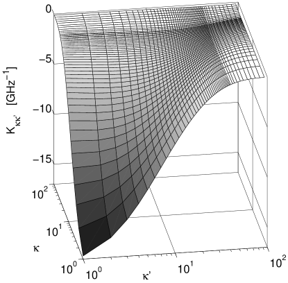
Figure 7: The reduced kernel matrix $\mathcal{K}_{\kappa\kappa^{\prime}}(E_{\mathrm{3B}})$ of Eq. (57), at low vibrational excitations $\kappa,\kappa^{\prime}<100$, for a $\nu_{\mathrm{ho}}=300$ kHz trap and a magnetic field strength of $B=158.1$ G. The transition from the linear to the connecting exponential mesh at $\kappa=N_{\mathrm{e}}=40$ is illustrated by the logarithmic scale of the axes associated with the vibrational quantum numbers $\kappa$ and $\kappa^{\prime}$ (cf. Eq. (105)). In the linear part ($0\leq\kappa,\kappa^{\prime}<N_{\mathrm{e}}$) the reduced kernel matrix was evaluated exactly using the results of Appendix B.3 while the approximation of Eq. (90) was used in the exponential part. The logarithmic scaling of the axes associated with $\kappa$ and $\kappa^{\prime}$ prevents the row $\kappa=0$ and the column $\kappa^{\prime}=0$ from being displayed.

The analogue of the momentum space Faddeev approach Gloeckle83 to three interacting Bose atoms in a trap involves, contrary to its free-space counterpart, discrete Faddeev equations represented by Eq. (57) in the separable potential approach. In the limit of low frequency trapping potentials, however, the basis set expansion leads to large kernel matrices and the numerical determination of the fixed points in Eq. (57) becomes impractical.

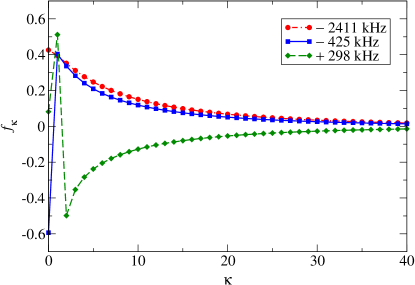
Figure 8: (Color online) Solutions $f_{\kappa}$ of the matrix equation (57), using the reduced kernel matrix shown in Fig. 7, versus the vibrational quantum number $\kappa$. The legends show the energies $E_{\mathrm{3B}}-\frac{6}{2}h\nu_{\mathrm{ho}}$ of the associated three-body levels of interacting ⁸⁵Rb atoms relative to the zero point energy of hypothetically non-interacting atoms in the $\nu_{\mathrm{ho}}=300$ kHz trap.

In order to demonstrate the orders of magnitude of the kernel matrix, we consider the projection of the form factor $g_{k}=\langle\varphi_{k}|g\rangle$ onto the harmonic oscillator basis. A simple calculation based on Eq. (17) shows that this projection is given by the formula:

$$g_{k}=\frac{4}{\pi^{1/4}}\frac{\zeta^{3/4}}{(1+\zeta)^{3/2}}\left(\frac{1-\zeta}{1+\zeta}\right)^{k}\sqrt{\frac{\Gamma(k+\frac{3}{2})}{\Gamma(k+1)}}.$$ (104)

Here we have introduced the dimensionless parameter $\zeta=\beta_{r}\sigma^{2}=\sigma^{2}\frac{1}{2}m\omega_{\mathrm{ho}}/\hbar$. The form factor thus decays like $g_{k}\sim e^{-2k\zeta}$ in the limit of large vibrational quantum numbers $k$. In the case of ⁸⁵Rb atoms the parameter $\zeta$ is on the order of $1.7\times 10^{-2}$ for a $\nu_{\mathrm{ho}}=300$ kHz atom trap, while it gets as small as $1.1\times 10^{-5}$ at a trap frequency of $\nu_{\mathrm{ho}}=200$ Hz. If we estimated the order of magnitude of a numerical cut-off $k_{\mathrm{max}}$, for instance, by supposing that the form factor is well represented when its value $g_{k}$ at $k=k_{\mathrm{max}}$ has decayed to $10^{-3}g_{0}$ we would require only $k_{\mathrm{max}}\approx 200$ basis states in the case of a 300 kHz trap. For a 1 kHz trap, however, this number would increase to $k_{\mathrm{max}}\approx 320000$. At low trap frequencies the kernel matrix would, therefore, become too large for a numerical solution of Eq. (57) to be practical.

To account for the discrete nature of the basis set expansion on the one hand and the exponential scaling of $g_{k}$, in the limit of large $k$, on the other hand, we have introduced a linear mesh of length $N_{\mathrm{e}}=40$ covering each of the lowest energy states, and a connecting exponential mesh of the same length containing the energetically higher states in the following way:

$$k_{j}=\left\{\begin{array}[]{lcc}j&:&0\leq j<N_{\mathrm{e}}\\ N_{\mathrm{e}}+\lfloor\ \left[e^{(j-N_{\mathrm{e}})\xi\delta}-1\right]/\xi\ \rfloor&:&N_{\mathrm{e}}\leq j<N_{\mathrm{t}}\\ \end{array}\right..$$ (105)

Here the symbol $\lfloor x\rfloor$ indicates the largest integer less than or equal to $x$, and $\xi\ll 1$ and $\delta$ are adjustable parameters. The parameter $\delta$ can be interpreted as the initial step size at the transition from the linear to the exponential mesh, i.e. $k_{N_{\mathrm{e}}+1}-k_{N_{\mathrm{e}}}\approx\delta$, which we have chosen as $\delta=2$. The parameter $\xi$ is fixed by the requirement $k_{N_{\mathrm{t}}-1}=k_{\mathrm{max}}$, leading to a transcendental equation for $\xi$ which can be solved numerically. In our applications the complete mesh then consisted of $N_{\mathrm{t}}=80$ points. We have generated an equivalent mesh for the sampling of the vibrational quantum number $\kappa_{j}$, resulting in an $80\times 80$ reduced kernel matrix $\mathcal{K}_{\kappa\kappa^{\prime}}(E_{\mathrm{3B}})$, which has been used for the numerical solution of Eq. (57). Figure (7) shows the reduced kernel matrix for a $\nu_{\mathrm{ho}}=300$ kHz atom trap at a magnetic field strength of $B=158.1$ G. The solutions $f_{\kappa}$ of Eq. (57) for the three lowest energetic three-body states obtained with the reduced kernel matrix of Fig. 7 are illustrated in Fig. 8.

B.6 Accuracy of the separable potential approach with respect to three-body energy spectra

The range of validity of our exact solutions to the three-body Faddeev equations is limited by the accuracy of the inter-atomic potentials. Figure 1 clearly demonstrates that the simultaneous adjustment of the separable potential of Appendix A to the scattering length of Eq. (1) and to the formula (7) for the binding energy of an alkali van der Waals molecule GF_PRA48 accurately describes both the measurements of Ref. Claussen03 and their ab initio theoretical predictions Kokkelmans_private04 . This accuracy of the approach with respect to the energies of ⁸⁵Rb₂ Feshbach molecules persists over a wide range of magnetic field strengths, extending from the position of the zero energy resonance of about 155 G up to 161 G, which is far beyond the range of validity of the universal formula (5). Our separable potential approach also recovers the excited state energy spectra for a pair of ⁸⁵Rb atoms in a 300 kHz trap which we have determined using a microscopic binary interaction $V(\mathbf{r})$ (see Fig. 1).

To demonstrate the validity of our separable potential approach also in its applications to three-body energy spectra, we shall compare its predictions to the ab initio binding energies of ⁴He₃ provided in Ref. Barletta01 . As the low static electric dipole polarizability of helium and the correspondingly small van der Waals coefficient of $C_{6}=1.461\,$a.u. Tang95 do not allow us to accurately recover the helium dimer binding energy from Eq. (7), we have used $E_{\mathrm{b}}/k_{\mathrm{B}}=-1.313\,$mK ($k_{\mathrm{B}}=1.3806505\times 10^{-23}$ J/K is the Boltzmann constant) in addition to the scattering length of $a=190.7\,$a.u. to adjust the parameters $A$ and $\sigma$ of the separable potential of Appendix A. These particular values of $a$ and $E_{\mathrm{b}}$ correspond to the Tang, Toennies and Yiu (TTY) helium dimer potential Tang95 reported in Ref. Barletta01 and determine the range parameter of the separable potential to be $\sigma=8.02\,$a.u.. This approach predicts the ⁴He₃ ground state energy to be $E_{1}^{\mathrm{sep}}/k_{\mathrm{B}}=-96.9\,$mK and for the excited Efimov state we obtain $E_{2}^{\mathrm{sep}}/k_{\mathrm{B}}=-2.09$ mK. These predictions only slightly overestimate the exact energies of $E_{1}^{\mathrm{TTY}}/k_{\mathrm{B}}=-126.4\,$mK and $E_{2}^{\mathrm{TTY}}/k_{\mathrm{B}}=-2.277\,$mK Barletta01 with relative deviations of 23 % and 8 %, respectively.

To study the uncertainties of our approach to determine the separable interaction, we have also performed a different adjustment of $V_{\mathrm{sep}}$ based on the requirement that its effective range $r_{\mathrm{eff}}^{\mathrm{sep}}=(4\sigma/\sqrt{\pi})[1-\sqrt{\pi}\sigma/(2a)]$ exactly recovers the effective range of $r_{\mathrm{eff}}=13.85\,$a.u. of the TTY potential in addition to the exact scattering length. This determines the range parameter to be $\sigma=6.31\,$a.u.. The associated potential $V_{\mathrm{sep}}$ yields $E_{\mathrm{b}}^{\mathrm{sep}}/k_{\mathrm{B}}=-1.285\,$mK for the helium dimer, while it predicts the trimer energies to be $E_{1}^{\mathrm{sep}}/k_{\mathrm{B}}=-142.6\,$mK and $E_{2}^{\mathrm{sep}}/k_{\mathrm{B}}=-2.36\,$mK with relative deviations from the ab initio results Barletta01 of 12 % and 4 %, respectively. Both adjustments of the separable potential thus lead to similar degrees of accuracy, which are comparable to the accuracy of the adiabatic hyper-spherical approach of Ref. Esry96 .

The small discrepancies between the predictions obtained from the different separable potentials and the ab initio calculations of Ref. Barletta01 indicate a remnant sensitivity of the trimer binding energies to properties of the microscopic binary interactions beyond those accounted for by the second order effective range expansion of the two-body scattering phase shift. Such corrections can, in principle, be exactly included in our calculations by taking advantage of the universal properties of low energy three-body spectra discussed, e.g., in Ref. Braaten03 . This presupposes, however, that one of the trimer binding energies is known either from experiment or from ab initio calculations. For instance, adjusting $V_{\mathrm{sep}}$ in such a way that it exactly recovers the trimer ground state energy of Ref. Barletta01 in addition to the binary scattering length yields $\sigma=6.79\,$a.u., which recovers the exact energy of the excited Efimov state reported in Ref. Barletta01 to a relative accuracy of 0.5 %. The studies of Ref. Gdanitz01 suggest, however, that the relatively small deviations between the ab initio and the different approximations employed in the separable potential approach may be physically insignificant due to the remaining uncertainties of even the comparatively well known helium dimer interaction potential.

References

- (1) L.H. Thomas, Phys. Rev. 47, 903 (1935).
- (2) V. Efimov, Phys. Lett. 33B, 563 (1970); Sov. J. Nucl. Phys. 12, 589 (1971); Comments Nucl. Part. Phys. 19, 271 (1990).
- (3) T.K. Lim, Sister K. Duffy, and W.C. Damert, Phys. Rev. Lett. 38, 341 (1977).
- (4) Th. Cornelius and W. Glöckle, J. Chem. Phys. 85, 3906 (1986).
- (5) B.D. Esry, C.D. Lin, and C.H. Greene, Phys. Rev. A 54, 394 (1996).
- (6) E.A. Kolganova, A.K. Motovilov, and S.A. Sofianos, J. Phys. B 31, 1279 (1998).
- (7) E. Nielsen, D.V. Fedorov, and A.S. Jensen, J. Phys. B 31, 4085 (1998).
- (8) T. González-Lezana, J. Rubayo-Soneira, S. Miret-Artés, F.A. Gianturco, G. Delgado-Barrio, and P. Villarreal, Phys. Rev. Lett. 82, 1648 (1999).
- (9) D. Blume and C.H. Greene, J. Chem. Phys. 112, 8053 (2000).
- (10) P. Barletta and A. Kievsky, Phys. Rev. A 64, 042514 (2001).
- (11) For a review, see A.S. Jensen, K. Riisager, D.V. Fedorov, and E. Garrido, Rev. Mod. Phys. 76, 215 (2004).
- (12) R.E. Grisenti, W. Schöllkopf, J.P. Toennies, G.C. Hegerfeldt, T. Köhler, and M. Stoll, Phys. Rev. Lett. 85, 2284 (2000).
- (13) W. Schöllkopf and J.P. Toennies, Science 266, 1345 (1994).
- (14) G.C. Hegerfeldt and T. Köhler, Phys. Rev. Lett. 84, 3215 (2000).
- (15) C.A. Regal, C. Ticknor, J.L. Bohn, and D.S. Jin, Nature (London) 424, 47 (2003).
- (16) K.E. Strecker, G.B. Partridge, and R.G. Hulet, Phys. Rev. Lett. 91, 080406 (2003).
- (17) J. Herbig, T. Kraemer, M. Mark, T. Weber, C. Chin, H.-C. Nägerl, and R. Grimm, Science 301, 1510 (2003).
- (18) S. Dürr, T. Volz, A. Marte, and G. Rempe, Phys. Rev. Lett. 92, 020406 (2004).
- (19) K. Xu, T. Mukaiyama, J.R. Abo-Shaeer, J.K. Chin, D. E. Miller, and W. Ketterle, Phys. Rev. Lett. 91, 210402 (2003).
- (20) S.T. Thompson, E. Hodby, and C.E. Wieman, Phys. Rev. Lett. 94, 020401 (2005).
- (21) D. Jaksch, V. Venturi, J.I. Cirac, C.J. Williams, and P. Zoller, Phys. Rev. Lett. 89, 040402 (2002).
- (22) M. Greiner, O. Mandel, T. Esslinger, T.W. Hänsch, and I. Bloch, Nature (London) 415, 39 (2002).
- (23) R. Long, T. Steinmetz, P. Hommelhoff, W. Hänsel, T.W. Hänsch, and J. Reichel, Phil. Trans. R. Soc. Lond. A 361, 1375 (2003).
- (24) T. Busch, B.-G. Englert, K. Rza̧żewski, and M. Wilkens, Found. Phys. 28, 549 (1998).
- (25) E. Tiesinga, C.J. Williams, F.H. Mies, and P.S. Julienne, Phys. Rev. A 61, 063416 (2000).
- (26) E.L. Bolda, E. Tiesinga, and P.S. Julienne, Phys. Rev. A 66, 013403 (2002).
- (27) M.T. Yamashita, R.S. Marques de Carvalho, L. Tomio, and T. Frederico, Phys. Rev. A 68, 012506 (2003).
- (28) E. Braaten and H.W. Hammer, cond-mat/0410417.
- (29) S. Jonsell, H. Heiselberg, and C.J. Pethick, Phys. Rev. Lett. 89, 250401 (2002).
- (30) D. Blume and C.H. Greene, Phys. Rev. A 66, 013601 (2002).
- (31) L.D. Faddeev, Soviet Phys. - JETP 12, 1014 (1961).
- (32) T. Köhler, T. Gasenzer, and K. Burnett, Phys. Rev. A 67, 013601 (2003).
- (33) T. Köhler, K. Góral, and T. Gasenzer, Phys. Rev. A 70, 023613 (2004).
- (34) B. Marcelis, E.G.M. van Kempen, B.J. Verhaar, and S.J.J.M.F. Kokkelmans, Phys. Rev. A 70, 012701 (2004).
- (35) C. Lovelace, Phys. Rev. 135, B 1225 (1964).
- (36) W. Sandhas, Acta Phys. Austriaca, Suppl. IX, 57 (1972).
- (37) V.B. Beliaev, Lectures on the Theory of Few-body systems, edited by K. Gaillard (Springer, Berlin, 1990).
- (38) F.H. Mies, E. Tiesinga, and P.S. Julienne, Phys. Rev. A 61, 022721 (2000).
- (39) K. Góral, T. Köhler, S.A. Gardiner, E. Tiesinga, and P.S. Julienne, J. Phys. B 37, 3457 (2004).
- (40) T. Köhler, T. Gasenzer, P.S. Julienne, and K. Burnett, Phys. Rev. Lett. 91, 230401 (2003).
- (41) J.M. Blatt and V.F. Weisskopf, Theoretical nuclear physics (Wiley, N.Y., 1952).
- (42) G.F. Gribakin and V.V. Flambaum, Phys. Rev. A 48, 546 (1993).
- (43) A similar formula was derived, independently of Ref. KGG04 , by D.S. Petrov [Phys. Rev. Lett. 93, 143201 (2004)].
- (44) Private communication from Servaas Kokkelmans.
- (45) E.G.M. van Kempen, S.J.J.M.F. Kokkelmans, D.J. Heinzen, and B.J. Verhaar, Phys. Rev. Lett. 88, 093201 (2002).
- (46) N.R. Claussen, S.J.J.M.F. Kokkelmans, S.T. Thompson, E.A. Donley, E. Hodby, and C.E. Wieman, Phys. Rev. A 67, 060701(R) (2003).
- (47) P. Soldán, M.T. Cvitas, J.M. Hutson, P. Honvault, and J.-M. Launay, Phys. Rev. Lett. 89, 153201 (2002).
- (48) D.S. Petrov, C. Salomon, and G.V. Shlyapnikov, Phys. Rev. Lett. 93, 090404 (2004).
- (49) C.A. Regal, M. Greiner, and D.S. Jin, Phys. Rev. Lett. 92, 083201 (2004).
- (50) T. Mukaiyama, J.R. Abo-Shaeer, K. Xu, J.K. Chin, and W. Ketterle, Phys. Rev. Lett. 92, 180402 (2004).
- (51) M. Bartenstein, A. Altmeyer, S. Riedl, R. Geursen, S. Jochim, C. Chin, J. Hecker Denschlag, R. Grimm, A. Simoni, E. Tiesinga, C.J. Williams, and P.S. Julienne, Phys. Rev. Lett. 94, 103201 (2005).
- (52) Private communication from C. Westbrook.
- (53) This terminology refers to the emblem of the Italian aristocratic family Borromeo, which consists of three rings interlinked in such a way that the remaining rings fall apart as soon as any one of the rings is removed.
- (54) J. Schwinger, Proc. Natl. Acad. Sci. U.S.A. 47, 122 (1961).
- (55) R.D. Amado and J.V. Noble, Phys. Rev. D 5, 1992 (1972).
- (56) W. Glöckle, The Quantum Mechanical Few-Body Problem (Springer, Berlin, 1983).
- (57) V.V. Flambaum, G.F. Gribakin, and C. Harabati, Phys. Rev. A 59, 1998 (1999).
- (58) B. Gao, Phys. Rev. A 62, 050702(R) (2000).
- (59) M.W. Zwierlein, C.A. Stan, C.H. Schunck, S.M.F. Raupach, S. Gupta, Z. Hadzibabic, and W. Ketterle, Phys. Rev. Lett. 91, 250401 (2003).
- (60) M.S. Chapman, C.R. Ekstrom, T.D. Hammond, R.A. Rubenstein, J. Schmiedmayer, S. Wehinger, and D.E. Pritchard, Phys. Rev. Lett. 74, 4783 (1995).
- (61) T. Köhler, E. Tiesinga, and P.S. Julienne, Phys. Rev. Lett. 94, 020402 (2005).
- (62) R.G. Newton, Scattering Theory of Waves and Particles (McGraw-Hill, N.Y., 1966).
- (63) P.M. Morse and H. Feshbach, Methods of Theoretical Physics, §12.3, p. 1662 (McGraw-Hill, N.Y., 1953).
- (64) A.G. Sitenko, Lectures in Scattering Theory (Pergamon Press, Oxford, 1971).
- (65) K.T. Tang, J.P. Toennies, and C.L. Yiu, Phys. Rev. Lett. 74, 1546 (1995).
- (66) E. Braaten and H.-W. Hammer, Phys. Rev. A 67, 042706 (2003).
- (67) R.J. Gdanitz, Mol. Phys. 99, 923 (2001).