Mechanisms of Electrical Conductivity in $Y_{1-x}Ca_{x}Ba_{2}Cu_{3}O_{6.1}$ System

Abstract

Systematic studies of transport properties in deoxygenated $Y_{1-x}Ca_{x}Ba_{2}Cu_{3}O_{6.1}$ series allowed to propose a diagram of conductivity mechanisms for this system. At intermediate temperature a variable range hopping (VRH) in 2 dimensions prevails. At lower temperature VRH in the presence of a Coulomb gap for smaller x and VRH in 2 dimensions for larger x are found. In a vicinity of superconductivity we observe conductivity proportional to $\sqrt{T}$. Thermally activated conductivity dominates at higher temperature. This diagram may be universal for the whole family of undoped high $T_{c}$ related cuprates.

High $T_{c}$ superconductors and their parent compounds remain ones of the most intriguing and not completely understood systems despite an impressive quantity of collected experimental material. All the different families of superconducting cuprates exhibit similar behavior as a function of holes doping to Cu-O planes[1, 2, 3]. Like in general case of the high $T_{c}$ related cuprates the undoped, deoxygenated $YBa_{2}Cu_{3}O_{6.1}$ is an antiferromagnetic insulator and increase in oxygen content provides holes to Cu-O planes, destroys static antiferromagnetic order, forces the insulator to metal transition and induces superconductivity[4]. There is a considerable number of reports on the effect of oxygen doping to the $YBa_{2}Cu_{3}O_{6+d}$ system[3, 4]. An alternative method is realized by divalent Ca substitution for trivalent Y, while the oxygen content remains constant[2, 5, 6, 7]. This chemical substitution resulting in the injection of holes into Cu-O planes allows to manipulate in carrier concentration quite precisely within the limit of Ca solubility. The deoxygenated $Y_{1-x}Ca_{x}Ba_{2}Cu_{3}O_{6.1}$ system exhibits superconductivity for higher Ca level[2, 5, 6, 7] and is characterized by a phase diagram[7] analogous to the diagram for $YBa_{2}Cu_{3}O_{6+d}$ with variable oxygen content[4].

A number of studies concerning electrical conductivity have been performed in order to understand the transport properties of the high $T_{c}$ related compounds and to investigate the phenomena occurring in the insulator to metal transition[8, 9, 10, 11, 12, 13, 14, 15]. For highly doped, superconducting samples a linear $\rho(T)$ (resistivity versus temperature) dependence with a positive slope in a normal state has been found[3], whereas for less doped samples different kinds of variable range hopping (VRH) conductivity have been observed[8, 9, 10, 11, 12, 13]. Electrical resistivity in the VRH mechanism follows the expression:

$${\rho}=\rho_{0}\exp(T/T_{0})^{-n}$$ (1)

where $n=1/4$ stands for VRH in 3 dimensions[16] observed e.g. in $Bi_{2}Sr_{2}Ca_{1-x}Y_{x}Cu_{2}O_{8+y}$ ceramics[8], $Bi_{2}Sr_{2}Ca_{1-x}Gd_{x}Cu_{2}O_{8+d}$ ceramics[9], both single crystals and ceramics of $La_{2-y}Sr_{y}Cu_{1-x}Li_{x}O_{4-\delta}$[10], $La_{2-x}Sr_{x}CuO_{4}$ ceramics[11], $La_{2}CuO_{4+\delta}$ single crystals[12] or $Y_{1-x}Pr_{x}Ba_{2}Cu_{3}O_{7}$ crystals[13]. The exponent $n$ equals $1/2$ for the VRH conductivity in the presence of a Coulomb gap or carrier interactions[17] which was found e. g. in $La_{2-x}Sr_{x}CuO_{4}$[11]. The exponent $n=1/3$ is a prediction for VRH in 2 dimensions[16], observed e.g. in $Bi_{2}Sr_{2}Ca_{1-x}Y_{x}Cu_{2}O_{8+y}$ ceramics[8] or $Bi_{2}Sr_{2}Ca_{1-x}Gd_{x}Cu_{2}O_{8+d}$ ceramics[9]. It was also found that thermally activated conductivity ($n=1$) is responsible for transport properties at higher temperature in $Bi_{2}Sr_{2}Ca_{1-x}Y_{x}Cu_{2}O_{8+y}$ ceramics[8] or in $La_{2}CuO_{4+\delta}$ single crystals[12]. The theoretical predictions for disordered metals[18] propose the expression

$$\sigma=\sigma_{0}+m\cdot\sqrt{T}$$ (2)

where $\sigma$ is static electrical conductivity. This relation was observed in $La_{1.85}Sr_{0.15}CuO_{4}$ ceramics with impurities[14]. Conductivity following the relation

$$\sigma\propto\ln(T)$$ (3)

indicates a weak localization in 2 dimensions or electron - electron interactions in the presence of disorder in 2 dimensions[18], found in $Nd_{1.85}Ce_{0.15}CuO_{4-\delta}$ in ab plane[15]. Luttinger liquid theory in two dimensions[19] predicts the following behavior of electrical resistivity:

$${\rho}\propto T^{1-4\alpha},$$ (4)

where $0\leq\alpha\leq\frac{1}{2}$ and $\alpha$ decreases in the transition from insulator to metal. To get a better insight into the conductivity mechanisms and systematize our knowledge concerning the insulator to metal and superconductor transition we performed measurements of electrical resistivity on a series of $Y_{1-x}Ca_{x}Ba_{2}Cu_{3}O_{6.1}$ samples.

$Y_{1-x}Ca_{x}Ba_{2}Cu_{3}O_{6+d}$ samples were prepared by the standard ceramic method. Subsequently, they were subjected to reduction in flowing Argon at 730 ${}^{o}C$ for 24 hours followed by slow cooling to room temperature. The oxygen content in the obtained samples amounted between 6.08 and 6.16. More details concerning preparation and characterization of the samples are given elsewhere[20]. Electrical resistivity measurements were performed with the four point contact method with reversing current direction in the temperature range of 6 K - 300 K. Electrical contacts were made of InAu alloy on mechanically cleaned sample surface. At each temperature, measurements with different electrical currents were made to verify if the resistivity is ohmic and to exclude the effect of heating or other non-linear phenomena. The applied current varied from 3 mA to the values lower than 1 $\mu A$ for the samples with the highest resistivity.

The measurements of electrical resistivity revealed a gradual modification of the transport properties with doping. As presented in Fig. 1 the system is insulating for x=0.00 and Ca substitution successively diminishes electrical resistivity. This is well reflected in the resistivity dependence as a function of Ca content at constant temperature (Fig. 1, inset). Superconductivity appears at x=0.3 with the onset temperature equal to 35 K, whereas is not visible above 6 K in the resistivity curve for x=0.26. The quantity of calcium at which superconductivity is induced was different than in the other reports[2, 6, 7]. The discrepancy in this field may be due to different methods of sample preparation, which can influence the existence of disorder or alter the ratio of Ca substituted into Y to substituted in Ba lattice positions. For example, the quoted reports[2, 6] concern the samples reduced by quenching in contrary to our method of preparation.

We will not discuss the metallic side of a metal-insulator transition, for which a linear $\rho(T)$ dependence is typically observed in high $T_{c}$ related cuprates. However, an ambiguous situation in the insulating side gave us motivation to verify the listed models of conductivity by drawing the data in appropriate scales. The plots of $\log(\rho)$ versus $T^{-\frac{1}{2}}$, $T^{-\frac{1}{3}}$ and $T^{-\frac{1}{4}}$ are presented in the Fig. 2 to consider if the VRH mechanisms occur. With the superficial analysis of the Fig. 2 it is difficult to confirm or exclude the existence of the mentioned mechanisms. In order to resolve which particular mechanism can dominate in different temperature and doping regions a normalized $\chi^{2}$ test was applied as the discussed relations were fitted to the experimental data. Different forms [21] of the expression (1): $\rho=\rho_{0}\exp((T/\tau)^{-1})$, $\rho=\rho_{0}^{\prime}\exp((T/T_{0}^{\prime})^{-\frac{1}{2}})$, $\rho=\rho_{0}^{\prime\prime}\exp((T/T_{0}^{\prime\prime})^{-\frac{1}{3}})$, $\rho=\rho_{0}^{\prime\prime\prime}\exp((T/T_{0}^{\prime\prime\prime})^{-\frac{1}{4}})$ and the power function (4) were fitted in different temperature ranges, particularly those, with visible linearity in appropriate scale. The relations (2) and (3) were fitted for $x\geq 0.16$, as for lower x they do not match the data visually. There was more than ten fitting ranges of temperature for each sample. In the Table 1, the fits with the lowest normalized $\chi^{2}$ values are indicated for the given temperature ranges. The proposed ranges in the Table 1 represent regions, where selected models of resistivity seem to be prevalent. This is reflected in larger differences between the smallest $\chi^{2}$ values for the proposed model and $\chi^{2}$ for the others.

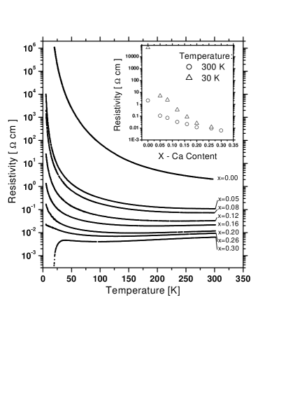
FIG. 1.: Electrical resistivity versus temperature for $Y_{1-x}Ca_{x}Ba_{2}Cu_{3}O_{6.1}$ samples. Inset: The resistivity at constant temperature as a function of Ca concentration

Before starting a discussion of the results from the Table 1 we will examine conditions for the existence of VRH[16, 17]. At the considered range of temperature the most probable hopping distance $R$ should be higher than the localization length $\xi$

$$R>\xi,$$ (5)

The evaluation of the inequality (5) leads to $T_{0}^{\prime}/4>T$, $T_{0}^{\prime\prime}/27>T$ and $T_{0}^{\prime\prime\prime}/50>T$ respectively for VRH in the presence of a Coulomb gap, VRH in two dimensions, and VRH in three dimensions. Hence, the parameters $T_{0}^{\prime}$, $T_{0}^{\prime\prime}$ and $T_{0}^{\prime\prime\prime}$ set necessary conditions for the temperature at which VRH can be accepted.

The analysis of the data from the Table 1 allowed to find some regularities in a behavior of electrical resistivity and we propose a diagram of the conductivity mechanisms for this system in the Fig. 3. It is postulated that different mechanisms are dominating in some temperature and doping regions. In reality, the different processes must coexist in certain areas of the diagram. Thus, it is purposeless to draw borders between the regions.

For the majority of investigated systems, we can distinguish three temperature ranges. In the intermediate range the existence of VRH in 2 dimensions ($n=1/3$) can be proposed. These regions are 26 K - 80 K for the specimen without Ca, 12 K - 70 K for samples with $x=0.05$ to 0.20 and 20 K to 80 K for the sample with $x=0.26$. The assumption (5) is fulfilled for the systems with $x=0.00$ to $x=0.16$ at the considered temperature. For the sample with $x=0.20$ VRH in 2 dimensions could be the case only below 25 K but at this temperature VRH in three dimensions will be prevalent ( Table 1 ). The condition (5) is failed for the systems with $x>0.20$.

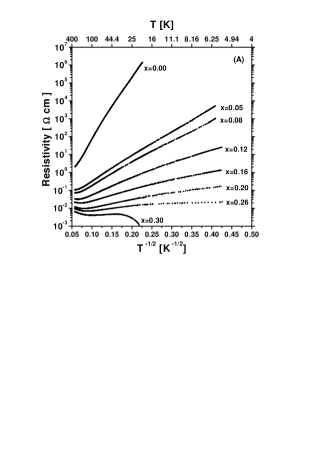
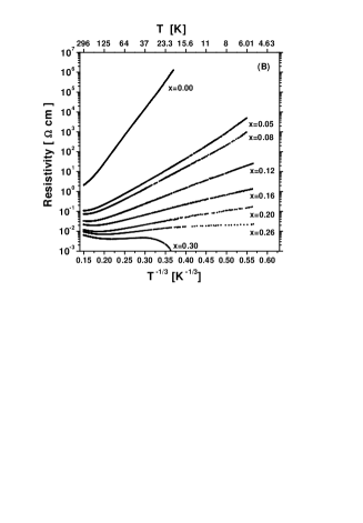
FIG. 2.: Electrical resistivity of the $Y_{1-x}Ca_{x}Ba_{2}Cu_{3}O_{6.1}$ system plotted in logarithmic scale as a function of: (A) $T^{-1/2}$, (B) $T^{-1/3}$, (C) $T^{-1/4}$.

The situation at lower temperature is more complex. For the samples with lower $x$ ($x=0.00$, $0.05$, $0.08$) the expression (1) with $n=1/2$ is preferred, indicating the VRH conduction in the presence of carrier interactions. For the system with $x=0.00$ this mechanism seems to occur at higher temperature and the region below 20 K was not considered due to some anomaly in electrical resistivity, origin of which was not clear. For the systems with higher Ca content, lower $\chi^{2}$ values were obtained for the relation (1) with $n=1/4$ signifying a VRH conduction in 3 dimensions. The condition (5) is satisfied for the low temperature ranges of fitting for $x\leq 0.2$. The low temperature data reveal that with increasing x, a crossover from VRH of interacting carriers to VRH of non-interacting carriers in three dimensions occurs. This result may be universal for a broader class of materials. Such a crossover was suggested previously for $La_{2-y}Sr_{y}CuO_{4}$ system[11] with an explanation that at higher $x$ the hole concentration increases sufficiently to provide screening down to the lowest temperature.

For lower $x$ in the diagram a crossover from VRH of interacting carriers to VRH in 3 dimensions appears with increasing temperature. For higher $x$ temperature induces a crossover in dimensionality. The question is why 2-dimensional hopping exists at higher temperature and is transformed to 3-dimensional with lowering the temperature. The $Y_{1-x}Ca_{x}Ba_{2}Cu_{3}O_{6.1}$ systems are regarded as quasi two-dimensional and the conductivity is principally related to the Cu-O planes. In consequence, it is not surprising that VRH in 2 dimensions is observed. At lower temperatures it is possible that the tunneling between the planes can compete with the motion within the planes. A crossover from 2-dimensional behavior to 3-dimensional at lower temperature have already been observed in some quasi two-dimensional materials[22].

In a case of the systems with higher level of doping the condition (5) excludes the existence of VRH in some regions. For the sample with $x=0.20$ the resistivity between 4 K and 30 K can be interpreted as a hopping in three dimensions. However, the range of 30 K to 70 K remains controversial. A breakdown of the VRH conductivity is well visible for the sample with $x=0.26$. In the considered temperature range of 20 K to 50 K the fit to the relation (2) describing the conductivity in disordered metals is characterized by the smallest $\chi^{2}$ value. As the coefficient $\sigma_{0}$ equals zero within experimental error, the relation (2) also corresponds to the predictions of the Luttinger liquid (4) with $\alpha=3/8$. For this sample the best fit among different types of hopping yielded the value of $T_{0}^{\prime\prime\prime}=8.9\cdot 10^{2}$ K for the VRH in 3 dimensions fitted in the range 20 K to 50 K. This value also excludes the existence of the VRH conductivity in the considered ranges of temperature. The resistivity at higher temperature is not discussed as the transition to the regime of positive $\rho(T)$ slope is quite close. At lower temperature a presence of some superconducting phase was detected in AC magnetic susceptibility[20] and therefore we restrict our consideration to the discussed temperature range.

It was difficult to discuss resistivity mechanisms above the transition to superconductivity for the sample with $x=0.3$. In this case, a range of negative $\rho(T)$ slope is limited by the transition to superconductivity on one side and by the positive $\rho(T)$ slope regime at higher temperature. The analysis in this restricted range seems unlikely to deliver any valuable information. The fits for the VRH mechanisms at the temperature of 45 K to 70 K allowed to estimate the parameters $T_{0}^{\prime\prime\prime}=35$ K for VRH in 3 dimensions and $T_{0}^{\prime\prime}=17$ K for VRH in 2 dimensions and VRH should be rejected because of the condition (5).

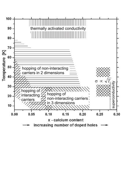
FIG. 3.: The proposed diagram of the conductivity mechanisms for $Y_{1-x}Ca_{x}Ba_{2}Cu_{3}O_{6.1}$ system.

At higher temperature a tendency to thermally activated conductivity appears. Although the $\chi^{2}$ values are the smallest for $n=1$ in these regions, the curves obtained by $\chi^{2}$ minimisation do not fit the data perfectly. This behavior probably cannot be described by pure relation (1) with $n=1$.

In summary, on the basis of systematical measurements of the electrical resistivity we have proposed a diagram of the conductivity mechanisms in the deoxygenated $Y_{1-x}Ca_{x}Ba_{2}Cu_{3}O_{6.1}$ system. At the intermediate temperature the existence of VRH in 2 dimensions is postulated, at lower temperature a crossover from VRH of interacting carriers to VRH of non-interacting carriers in 3 dimensions is observed with doping. For the highly doped samples a hopping conductivity should be excluded while the relation proposed for highly disordered metals or for the Luttinger liquid matches the experimental data better than the other relations do. Evidence for thermally activated conductivity is found at higher temperature. This diagram may be universal for the insulator-metal transitions induced by doping in different families of the high $T_{c}$ cuprates.

The authors are grateful to T. Plackowski and Z. Tomkowicz for help in experimental part of this work. P.S. appreciates the discussions with Prof. J. Spałek.

TABLE I.: The best fits to the experimental data for the selected ranges of temperature. For the relation (1) an exponent $n$ and the values of $T_{0}^{\prime}$, $T_{0}^{\prime\prime}$ and $T_{0}^{\prime\prime\prime}$ for VRH conductivity are given. In a case that the condition (5) is not fulfilled within the whole fitting range, the temperature satisfying this condition is marked.

Investigated sample		Temperature range of fitting
		Best fit
$YBa_{2}Cu_{3}O_{6.16}$	20 K - 60 K	26 K - 80 K	180 K - 300 K
	$n=1/2$, $T_{0}^{\prime}=5.6\cdot 10^{3}$K	$n=1/3$, $T_{0}^{\prime\prime}=2.4\cdot 10^{5}$ K	$n=1$
$Y_{0.95}Ca_{0.05}Ba_{2}Cu_{3}O_{6.15}$	6 K - 30 K	12 K - 70 K	80 K - 200 K
	$n=1/2$, $T_{0}^{\prime}=9.2\cdot 10^{2}$ K	$n=1/3$, $T_{0}^{\prime\prime}=2.1\cdot 10^{4}$ K	$n=1$
$Y_{0.92}Ca_{0.08}Ba_{2}Cu_{3}O_{6.08}$	6 K - 30 K	12 K - 70 K	80 K - 200 K
	$n=1/2$, $T_{0}^{\prime}=6.8\cdot 10^{2}$ K	$n=1/3$, $T_{0}^{\prime\prime}=1.6\cdot 10^{4}$ K	$n=1$
$Y_{0.88}Ca_{0.12}Ba_{2}Cu_{3}O_{6.09}$	6 K - 30 K	12 K - 70 K	80 K - 200 K
	$n=1/4$, $T_{0}^{\prime\prime\prime}=1.3\cdot 10^{5}$ K	$n=1/3$, $T_{0}^{\prime\prime}=6.1\cdot 10^{3}$ K	$n=1$
$Y_{0.84}Ca_{0.16}Ba_{2}Cu_{3}O_{6.09}$	6 K - 30 K	12 K - 70 K	80 K - 160 K
	$n=1/4$, $T_{0}^{\prime\prime\prime}=2.3\cdot 10^{4}$ K	$n=1/3$, $T_{0}^{\prime\prime}=1.8\cdot 10^{3}$ K	$n=1$
$Y_{0.80}Ca_{0.20}Ba_{2}Cu_{3}O_{6.11}$	6 K - 30 K	12 K - 70 K	80 K - 120 K
	$n=1/4$, $T_{0}^{\prime\prime\prime}=5.3\cdot 10^{3}$ K	$n=1/3$, $T_{0}^{\prime\prime}=6.7\cdot 10^{2}$ K	$n=1$
		condition (5): $T<25$ K
$Y_{0.74}Ca_{0.26}Ba_{2}Cu_{3}O_{6.11}$	20 K - 50 K	-	-
	relation (2): $\sigma=\sigma_{0}+m\cdot\sqrt{T}$

REFERENCES

- [1] M. R. Presland et al., Physica C 176, 95 (1991).
- [2] J. L. Tallon et al., Phys. Rev. B 51, 12911 (1995).
- [3] M. Cyrot, D. Pavuna, Introduction to Superconductivity and High-Tc Materials, World Scientific, 1992.
- [4] D. C. Johnston et al., Physica C 153-155, 572 (1988).
- [5] E. M. McCarron, M. K. Crawford and J. B. Parise, J. Solid State Chem. 78, 192 (1989).
- [6] R. S. Liu et al., Solid State Commun. 76, 679 (1990).
- [7] H. Casalta et al., Physica C 204, 331 (1993).
- [8] P. Mandal et al., Phys. Rev. B 43, 13102 (1991).
- [9] B. Jayaram et al., Phys. Rev. B 43, 5444 (1991).
- [10] M. A. Kastner et al., Phys. Rev. B 37, 111 (1988).
- [11] B. Ellman et al., Phys. Rev. B 39, 9012 (1989).
- [12] B.I. Belevcev, N. V. Dalakova, A. C. Panfilov, Fizika Nizkix Temperatur 23, 375 (1997).
- [13] Wu Jiang et al., Phys Rev B 49, 690 (1994).
- [14] M. Z. Cieplak et al., Phys. Rev. B 46, 5536 (1992).
- [15] A. Kussmaul et al., Physica C 177, 415 (1991).
- [16] N. F. Mott, J. H. Davies, Electronic Processes in Non-Crystalline Materials, Oxford University Press, 1979.
- [17] B. I. Shklovskii, A. L. Efros, Electronic Properties of Doped Semiconductors, Springer-Verlag, Berlin, 1984.
- [18] P.A. Lee and T.V. Ramakrishnan, Rev. Mod. Phys. 57, 287 (1985).
- [19] K. Byczuk, J. Spałek, W. Wójcik, Acta Physica Polonica B 29, 3871 (1998).
- [20] P. Starowicz et al., Physica C 363, 80 (2001).
- [21] The symbol from the Equation (1) corresponds to , , and respectively for , , and .
- [22] T. Valla et al., Nature 417, 627 (2002).