A Mechanism for Pockets of Predictability in Complex Adaptive Systems

Abstract

We document a mechanism operating in complex adaptive systems leading to dynamical pockets of predictability (“prediction days”), in which agents collectively take predetermined courses of action, transiently decoupled from past history. We demonstrate and test it out-of-sample on synthetic minority and majority games as well as on real financial time series. The surprising large frequency of these prediction days implies a collective organization of agents and of their strategies which condense into transitional herding regimes.

The concept of complex adaptive feedbacks is increasingly used to understand the earth climate, immune systems, nervous systems, multicellular organisms, insect societies, ecologies, economies, human societies, stock markets, distributed computing systems, large-scale communication networks. A trademark of such systems is the occurrence of extreme events, which are in general believed to be unpredictable Karplus . However, a few recent works suggest a degree of predictability in some cases, for instance associated with transient herding phases in the population of agents JSL , or signaled by empirical patterns Lo . Previous attempts to examine the predictability of large future changes have used models of evolving agents competing for a limited resource Farmer ; Lamper . These agents have memory and use complex (possibly learning) algorithms. Although they can show predictive power, the complexity of agent-based models has not provided an understanding of the factors that lead to the predictions except to say that they are a consequence of the information incoded in the system’s global state Lamper . This is particularly problematic for concrete applications for which predictions become credible and usable only when based upon a sound physical understanding of their limitations and of the range and likelihood of competing scenarios.

Let us consider a generic multi-agent system comprising a population of $N$ agents of which less than half of the agents can win at each time step. Each agent will thus seek to be in the minority group. In Cavagna , it is was shown that, for such Minority Games (MG), it is the information common to all the agents, rather than the feedback of their actions onto the price, which determines the dynamics of the game. Here, we extend this observation and show the surprising fact that, for minority as well as for majority games $-game , at certain times, the information contained in a few last moves becomes irrelevant in the agents’ decision making, a situation that we refer to as “decoupling.” This leads to dynamical pockets of predictability, with agents taking a predetermined course of action which is decoupled from the price history of the system over a finite number of time steps. We are able to unveil the origin of these pockets of predictability that we test out-of-sample on synthetic as well as on real financial time series using a suitably calibrated agent-based model.

Our results apply to systems which can be represented by agent-based models, in which each agent $i$ has a finite memory over $m_{i}$ time steps fed to his $s_{i}$ strategies. Without significant loss of generality, we follow most previous models BookMG and assume that $m_{i}=m$ and $s_{i}=s$ for all agents. At each time step $t$, each of the $N$ agents makes either a decision $a^{\mu_{m}}_{i}(t)=\pm 1$ (yes or no, itinary A or B, buy or sell, etc.) using his best (among the $s$) strategy or does nothing, based on the available information of the last $m$ time steps. The available common information $\mu_{m}(t)$ at time $t$ is the series of past total actions of all the agents over the last $m$ time steps

$$\mu_{m}(t)=\{{1+{\rm sign}[A^{\mu}(k)]\over 2};k=t-m+1,...,t\}~{},$$ (1)

where $A^{\mu}(k)=\sum_{i}a^{\mu}_{i}(k)$. Thus, $\mu_{m}(t)$ is a string of $m$ binary digits $0$ (a majority of agents played $-1$) or $1$ (a majority of agents played $+1$). A strategy is a mapping from the $2^{m}$ possible price histories onto the two possible decisions. An example of a strategy with $m=3$ is

$$\{000\to 0;001\to 0;010\to 1;011\to 0;$$

$$100\to 1;101\to 0;110\to 1;111\to 0\}~{}.$$ (2)

Different payoffs of strategies define different mechanisms and apply to distinct situations. The standard MG corresponds to the payoff $g_{j}(t)=-a_{j}(t)A(t)$: if a strategy $j$ is in the minority ($a_{j}(t)A(t)<0$), it is rewarded. In other words, agents in the MG try to be anti-imitative. Another payoff, for instance motivated by real financial markets, is $-game ; Giardina $g_{j}(t)=a_{j}(t-1)A(t)$. In this case, the price is an increasing function of the excess demand $A(t)$ and the payoff reflects the tendency for a strategy to win if it has anticipated correctly the next market move. Our results apply equally well to these two as well as other payoffs.

Given the common information $\mu_{m}(t)$ at time $t$, we define the process of decoupling of a strategy as follows:
$\bullet$ A strategy $s_{j}$ is called $n-$time steps decoupled conditioned on $\mu_{m}(t)$ if the action $s_{j}(\mu_{m}(t+n+1))$ does not depend on $\mu_{m}(t+1),...,\mu_{m}(t+n)$.
$\bullet$ A strategy $s_{i}(\mu_{m}(t+n+1))$, whose action at time $t+n+1$ depends on at least one of the outcomes of $\mu_{m}(t+1),...,\mu_{m}(t+n)$, is coupled to the information flow.
As an example, consider the strategy (2). This strategy is one-time step decoupled conditioned on $\mu_{3}(t)=000$ or $\mu_{3}(t)=100$ since, in both realisations $\mu_{3}(t+1)=000$ or $\mu_{3}(t+1)=001$, the strategy’s action is $0$ at time $t+2$. More generally, a strategy $s$ with $m=3$ is one-step decoupled conditioned on the common information $\mu_{3}(t)=abc$ if $s(bc0)=s(bc1)$. It is then automatically decoupled conditioned on $\mu_{3}(t)={\bar{a}}bc$ where ${\bar{a}}=1$ if $a=0$ and ${\bar{a}}=0$ if $a=1$. The fraction of one-step decoupled strategies conditioned on having only one pair $(abc,{\bar{a}}bc)$ decoupled is ${4\choose 1}2^{-4}=1/4$, since there are four possible pairs $(bc)$ each having a probability $1/2$ that $s(bc0)=s(bc1)$. The strategy $s$ is two-step decoupled conditioned on $\mu_{3}(t)=abc$ if $s(c00)=s(c01)=s(c10)=s(c11)$. For the general $m$ memory case, a strategy is one-step decoupled conditioned on $\mu_{m}(t)=c_{1}c_{2}...c_{m}$ if $s(c_{2}...c_{m}0)=s(c_{2}...c_{m}1)$. The fraction of one-step decoupled strategies on at least one pair of histories is $1-2^{-2^{m-1}}$, which is one minus the probability that none among the number $2^{m-1}$ of $(m-1)$-plets obey $s(c_{2}...c_{m}0)=s(c_{2}...c_{m}1)$. A strategy is $n$-step decoupled (with $n\leq m$) if $s(c_{n+1}...c_{m}\{\mu_{n}\})$ is independent of all possible $2^{n}$ histories $\{\mu_{n}\}$ of string length $n$. The fraction of $n$-step decoupled strategies conditioned on any $(m-n)$-plets only is $1-(1-2^{-(2^{n}-1)})^{2^{m-n}}$, because $2^{-(2^{n}-1)}$ is the probability for a given history to be $n$-step decoupled, thus $1-2^{-(2^{n}-1)})$ is the probability to be $n$-step coupled and there are $2^{m-n}$ $(m-n)$-plets. Thus, as soon as $n$ becomes larger than $\approx\ln_{2}(m)$, the $n$-step decoupled strategies become extremely rare.

What is interesting about decoupled strategies is that they open the possibility that one can predict with certaintynote1 the future global action in two (or more) time steps ahead without having to know it at the next time step. This occurs when a majority of agents use decoupled strategies which combine to a majority action. Indeed, the common action of all the agents at time $t+n+1$ can be written as the sum of two contributions, one stemming from coupled and the other from decoupled strategies (conditioned on the history ${\mu_{m}}(t)$):

$$A^{{\mu_{m}}(t)}\equiv A_{\rm coupled}^{{\mu_{m}}(t)}+A_{\rm decoupled}^{{\mu_{m}}(t)}~{}.$$ (3)

The condition for certain predictability $n$ time steps ahead is therefore

$$|A_{\rm decoupled}^{{\mu_{m}}(t)}(t+n+1)|>N/2~{}.$$ (4)

We call these times when condition (4) is met “prediction days.”

It is interesting to estimate the frequency of such prediction days that would be obtained if strategies and histories were randomly chosen. Let us first estimate the probability ${\rm Pr}_{1}$ that a given agent is $n$-step decoupled. This is the probability that he is active and that his best strategy is $n$-step decoupled. The former is a fixed finite fraction $0<\eta<1$ of time. The probability that his best strategy is $n$-step decoupled is the product of the probability that his best strategy belongs to the set of possibly $n$-step decoupled strategies times the probability that the present history is decoupling for that strategy. The former is $1-(1-2^{-(2^{n}-1)})^{2^{m-n}}$ as shown above. The later is $1/2^{2^{n}-1}$, which is the probability for $2^{n}$ values $s(c_{n+1}...c_{m}\{\mu_{n}\})$ to be equal for all $2^{n}$ histories $\{\mu_{n}\}$. This gives

$${\rm Pr}_{1}(m,n)=\eta\left[1-\left(1-{1\over 2^{2^{n}-1}}\right)^{2^{m-n}}\right]{1\over 2^{2^{n}-1}}.$$

We have for instance ${\rm Pr}_{1}(m=3,n=1)=3\eta/8$; ${\rm Pr}_{1}(m=3,n=2)=11\eta/216$, ${\rm Pr}_{1}(m\to+\infty,n=1)\to\eta/2$ from below, and ${\rm Pr}_{1}(m,n)<\eta/2$ for all $n\leq m$.

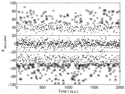
Figure 1: $A_{\rm decoupled}$ defined in (3) as a function of time for the MG with $N=101,s=12,m=3$. Circles indicate one-step prediction days, crosses are the subset of days starting a run of two or more consecutive one-step prediction days.

Assuming complete incoherence between the strategies and histories, the probability ${\rm Pr}_{\rm pred}$ that condition (4) is met is

$${\rm Pr}_{\rm pred}=2\sum_{D={N\over 2}}^{N}[{\rm Pr}_{1}]^{D}\sum_{D_{+}>{D\over 2}+{N\over 4}}^{D}{D\choose D_{+}}{1\over 2^{D}}$$ (5)

where $D$ is the number of active decoupled agents and $D_{+}$ is the number among them who take a positive step. The factor $2$ comes from the two possible signs of $A_{\rm decoupled}^{{\mu_{m}}(t)}$. The lower bound ${D\over 2}+{N\over 4}<D_{+}$ in the second sum ensures that condition (4) is obeyed. The lower bound $D=N/2$ in the first sum expresses the obvious fact that condition (4) is met when the number of decoupled agents is at least $N/2$ (this lower bound is reached when they all agree). Now, the second sum is obviously bounded from above by $1$. This yields

$${\rm Pr}_{\rm pred}<{2{\rm Pr}_{1}^{N/2}\over 1-{\rm Pr}_{1}}<{4\over 2-\eta}\left({\eta\over 2}\right)^{N/2}<{4\over 2^{N/2}}~{},$$ (6)

where the two last bounds use the fact that ${\rm Pr}_{1}(m,n)<\eta/2<1/2$ for all $n,m$. This result (6) shows that in this scenario, as soon as one considers populations of agents of the order of a few tens or more, the probability to find a prediction day is exceedingly small. In our simulations below, we have used $N=25$ and $N=101$, which gives respectively ${\rm Pr}_{\rm pred}<7\cdot 10^{-4}$ and ${\rm Pr}_{\rm pred}<2.5\cdot 10^{-15}$.

Figure 1 shows a typical time series of $A_{\rm decoupled}$ as a function of time for the standard MG with $N=101,s=12,m=3$. When strategies are randomized at each time step, there are no prediction day as espected from our above estimated probability (6) which applies to this case and $A_{\rm decoupled}$ remains confined around zero within the strip delineated by the two horizontal lines at $\pm 20$. In constrast, Fig. 1 shows a surprisingly large fraction $\rho_{\rm pred}=17.5\%$ for one-step prediction days and $3.5\%$ for two or more consecutive days which are predictive. This implies that the prediction days result from a collective organization of agents and of their strategies which condense into a herding regime characterized by a rather strong synchronization of both their decoupling and of their action conditioned on decoupling.

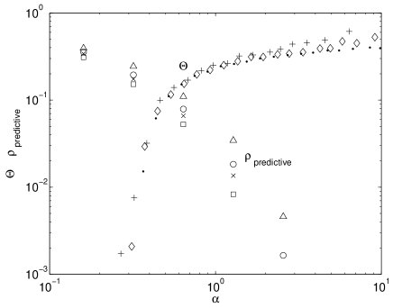
Figure 2: $\theta\equiv{\overline{\langle{\rm sign}[A]\rangle^{2}}}$ and the frequency of predictive days, $\rho_{\rm pred}$ versus $\alpha\equiv 2^{m}/N$. Simulations for $\theta$ were done with $s=2$, $m=5$ ($+$), $m=6$ (diamonds), $m=7$ (black dots). Simulations for $\rho_{\rm predictive}$ were done with $N=25$, $s=7$ (squares), $s=8$ (crosses), $s=9$ (circles), $s=12$ (triangles).

By scanning different values for the number $s$ of strategies per agent and for the memory $m$, figure 2 shows that the new phenomenon discovered here is a robust property of MG. We also compare the occurrence of our prediction days with a measure of predictability $\theta\equiv{\overline{\langle{\rm sign}[A^{\mu}]\rangle^{2}}}$ introduced by Savit et al. CM , where $\langle{\rm sign}[A^{\mu}]\rangle$ is the time-average of the collective action conditioned upon the occurrence of a given history $\mu$, while the upper bar denotes the average over all possible histories. Previous works (see also figure 2) have shown that there is a critical value $\alpha_{c}\approx 0.35$ (where $\alpha\equiv 2^{m}/N$) such that $\theta$ goes from non-zero (statistically predictable regime) for $\alpha>\alpha_{c}$ to zero (statistically unpredictable regime) for $\alpha<\alpha_{c}$. Our simulations illustrate a case where our prediction days are in fact more frequent in the previously classified “statistically unpredictable” regime, showing that we are dealing with a fundamentally different property. Note that $\rho_{\rm pred}$ grows as $\alpha$ decreases, i.e., when $m$ decreases and $N$ increases, in blatant contradiction with the expectations (5) assuming incoherent and random choices. Again, this reinforces the evidence that the prediction days results from a special herding organization of the strategies in conjunction with the realized histories.

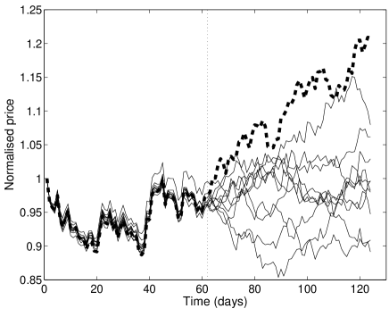
Figure 3: Fat dashed line: Nasdaq Composite price history (black-box game) as a function of time (days); thin solid lines: ten predicted price trajectories obtained from the third-party games. The first in-sample 61 days are used to calibrate ten third-party games. The days 62-123 are out-of-sample. The third-party games make a poor job at predicting the out-of-sample prices of the Nasdaq Composite index, while table 1 shows that they predict specific pockets of predictability associated with forecasted “prediction days” (see text).

A major objection could be raised that the information required for identifying a prediction day includes, not only the common knowledge of past history but, the active strategies used by the agents, which are in general unobservable. Actually, it is possible to retrieve sufficient information on the strategies by using a methodology derived from Lamper et al. Lamper , which allows one to invert a time series of observable collective action $A(t)$ generated by a black-box game to obtain an ensemble of so-called third-party games by optimizing a measure of the matching between the observed time series and synthetic time series generated with the third-party games fut . It is then possible to identify the prediction days in the third-party games. To quantify how these prediction days by third-party games provide a forecast for the black-box game, we use as a metric the success rate to forecast the correct sign of the global action $A$ on a prediction day identified by the third-party games compared with the success rate on other days. In particular, we monitor how these success rates vary with the predicted amplitude of $A_{\rm decoupled}$, since expression (3) shows that the larger it is, the more predictable is the global action. We find that, for both the MG as well as for the majority $-game $-game , the former success rate shows the predicted behavior of increasing monotonically from 50% for small $A_{\rm decoupled}$ to 100% for large $A_{\rm decoupled}$. In contrast, we do not observe any significant prediction skill above 50% on non-prediction days. Rather than reporting these results in details on synthetic MG and $ games, we now show that our method works for real complex system of competing agents, and we take the stock market as a significant application. We use the return time series of the Nasdaq Composite index as the proxy for the global action $A(t)$, whose price trajectory is shown in figure 3. We construct ten third-party $-games (with the same parameters but different realizations of strategies endowed to the agents) calibrated on the first $61$ daily returns to the left of the vertical dashed line in figure 3. We then feed to these third-party games the realized returns of the Nasdaq Composite and compare their predictions with the realized price. The predictions are issued at each close of the day for the next close, all third-party games being unchanged for the test over the second part of the time period from $t=62$ to $123$. Among the $62$ out-of-sample days, we monitor our ten third-party games to detect a prediction day (we use a voting process among the ten third-party games to obtain better robustness), according to the active strategies and the predicted one-step ahead history for the next close. Conditioned on the detection of a prediction day, we issue a prediction of the sign of the next day return and compare it with the realized market return. The performance of this prediction scheme is reported in table 1 which is typical of our results. The important point is that the success rate ($\%$ in the table) increases with the predicted amplitude of $A_{\rm decoupled}$, as for the synthetic MG and $-game mentioned above.

$|A|$	0	0.5	1	1.5	2	2.5	3	3.5	4	4.5
%	53	61	67	65	82	70	67	67	100	100
Nb	62	49	39	23	17	10	6	3	2	1

Table 1: Out-of-sample success rate % (second row) using different thresholds for the predicted global decoupled action (first row) of the third-party $-games calibrated to the Nasdaq Composite index. ${\rm Nb}$ (third row) is the number of days from $t=62$ to $123$ which have their predicted global decoupled action $|A_{\rm decoupled}|$ larger than the value indicated in the first row.

In contrast, the use of the third-party games for predicting each day the sign of the next return fails, as can be seen from the ten trajectories in the out-of-sample time interval. Our method has thus identified pockets of predictability in the Nasdaq index associated with the prediction of ensembles of decoupled strategies predicted by the third-party games.

References

- (1) W.J. Karplus, The Heavens are Falling: The Scientific Prediction of Catastrophes in Our Time (New York: Plenum Press, 1992).
- (2) A. Johansen et al., J. Risk 1, 5 (1999).
- (3) A. Lo et al., J. Finance 55, 1705 (2000).
- (4) Farmer, J.D., Industrial and Corporate Change 11, 895 (2002).
- (5) D. Lamper et al., Phys. Rev. Lett. 88, 017902 (2002).
- (6) A. Cavagna, Phys. Rev. E , 59, R3783 (1999).
- (7) D. Challet, M. Marsili and Y.-C. Zhang, Minority Games: Interacting Agents In Financial Markets (Oxford University Press, 2004).
- (8) J.V. Andersen and D. Sornette, Eur. Phys. J. B 31, 141 (2003).
- (9) I. Giardina and J.-P. Bouchaud, Eur. Phys. J. B 31, 421 (2003).
- (10) Ignoring the indeterminacy that comes from strategies that are degenerate in score as well ignoring any change in score between time and .
- (11) R. Savit et al., Phys. Rev. Lett. 82, 2203 (1999); D. Challet and M. Marsili, Phys. Rev. E 62, 1862 (2000).
- (12) The details of the method will be reported elsewhere.