Re-parameterization Invariance in Fractional Flux Periodicity

Abstract

We analyze a common feature of a nontrivial fractional flux periodicity in two-dimensional systems. We demonstrate that an addition of fractional flux can be absorbed into re-parameterization of quantum numbers. For an exact fractional periodicity, all the electronic states undergo the re-parameterization, whereas for an approximate periodicity valid in a large system, only the states near the Fermi level are involved in the re-parameterization.

The Aharonov-Bohm (AB) effect [1, 2] is one of the direct manifestations of the quantum nature of electrons. The interference pattern obtained in an AB experiment shows that a single electron wave function has the fundamental unit of magnetic flux, $\Phi_{0}=hc/e$. The AB effect has important physical consequences also in solid state physics. For example, an equilibrium persistent current [3, 4], which is a derivative of the ground state energy $E_{0}(\Phi)$ by the threading flux $\Phi$, $I_{\rm pc}=-\frac{\partial E_{0}(\Phi)}{\partial\Phi}$ in mesoscopic metallic rings is observed experimentally [5, 6, 7]. Coherence effects between electrons appear in $I_{\rm pc}$ as functions of threading flux. Since the ground state of materials consists of many electrons, the AB effect can lead to physical results due to the coherence between the electrons. One of the interesting coherence effects is a fractional flux periodicity in the ground state energy. The fractional flux periodicity means that for $\Delta=\Phi_{0}/Z$ ($Z$ is an integer), $E_{0}(\Phi+\Delta)=E_{0}(\Phi)$ holds exactly or in a certain limit for any $\Phi$. There are several theoretical studies on the fractional flux periodicity. Cheung et al. [8] found that a finite length cylinder with a specific aspect ratio exhibits the fractional flux periodicity in the persistent currents. The same configuration obtained with a magnetic field applied perpendicular to the cylindrical surface was shown to have a fractional flux periodicity by Choi and Yi [9]. Such cylinders are composed of a square lattice. In addition to these cylinders, the torus geometry composed of a square lattice exhibits the fractional flux periodicity, depending on the twist around the torus axis and the aspect ratio [10, 11]. Similarly to a square lattice, a honeycomb lattice can also show the fractional flux periodicity. We found that an armchair carbon nanotube with heavy doping can exhibit the fractional flux periodicity [12]. Even though all these systems showing a fractional flux periodicity are two-dimensional (2D) systems, common features for the fractional periodicity have not yet been clarified.

If all electronic states for $\Phi$ and $\Phi+\Delta$ have the same energy in one-to-one correspondence, the AB effect can occur. However, when we plot one electron energy as a function of magnetic field, each electron state for $\Phi$ does not always correspond to the state for $\Phi+\Delta$ with the same energy; the state for $\Phi+\Delta$ with the same energy may come from the other state for $\Phi$. In this case, we can specify the states for $\Phi+\Delta$ by re-parameterizing the quantum numbers of the states for $\Phi$. A general question is whether there is such a re-parametrizing operation as a function of magnetic field. In this context, we have shown for some fractional periodic systems that there is a re-parametrizing operation that gives an invariance (re-parametrization invariance) for a single-electron energy. There are two types of fractional flux periodicity; one is an exact one, while the other is achieved in a limit of a large system. For both types of fractional flux periodicity, in general, an addition of fractional flux can be recognized as a re-parameterization of quantum numbers, as we will discuss later on a twisted torus [10, 11] and a cylinder [8] composed of a square lattice. For the exact periodicity, all the electronic states for $\Phi$ and $\Phi+\Delta$ are in one-to-one correspondence by the re-parameterization, whereas for the approximate periodicity, only the states near the Fermi level are involved in the re-parameterization.

We first analyze the flux periodicity of a twisted torus composed of a square lattice considered in refs. SKS,SKS2. We consider a nearest-neighbor tight-binding model on a torus, with the hopping integral $t$ between nearest-neighbor sites. Let $N$ and $Q$ denote the numbers of lattice sites around and along the torus axis, respectively, and let $\delta N$ denote the twist along the torus axis. The energy eigenvalue of the system is

$$E_{\mu_{1}\mu_{2}}(\Phi)=-2t\left\{\cos\left(\frac{2\pi\mu_{1}}{N}\right)\right.$$

$$\ \ \ \ +\left.\cos\frac{2\pi}{Q}\left(\mu_{2}-\frac{\delta N}{N}\mu_{1}-\frac{\Phi}{\Phi_{0}}\right)\right\},$$ (1)

where $\mu_{1}$ and $\mu_{2}$ are integer quantum numbers, taking the values $\mu_{1}=1,\cdots,N$, $\mu_{2}=1,\cdots Q$. Because $E_{\mu_{1},\mu_{2}}=E_{\mu_{1}+N,\mu_{2}+\delta N}=E_{\mu_{1},\mu_{2}+Q}$, the region for the integers $\mu_{1}$ and $\mu_{2}$ can be taken as any $N$ and $Q$ consecutive integers, respectively. When the Fermi level is fixed at $E_{F}=0$, $E_{0}(\Phi)$ can be expressed as $E_{0}(\Phi)=\sum^{\prime}_{\mu_{1}\mu_{2}}E_{\mu_{1}\mu_{2}}(\Phi)$, where $\sum^{\prime}$ is a summation over the states with negative energy eigenvalues $E_{\mu_{1}\mu_{2}}(\Phi)<0$. We can rewrite it as

$$E_{0}(\Phi) = -\frac{1}{2}\sum_{\mu_{1}\mu_{2}}\left(\left|E_{\mu_{1}\mu_{2}}(\Phi)\right|-E_{\mu_{1}\mu_{2}}(\Phi)\right)$$ (2)

$$= -t\sum_{\mu_{1},\mu_{2}}\left|\cos\left(\frac{2\pi\mu_{1}}{N}\right)\right.$$

$$\ \ \ \ \ \left.+\cos\frac{2\pi}{Q}\left(\mu_{2}-\frac{\delta N}{N}\mu_{1}-\frac{\Phi}{\Phi_{0}}\right)\right|,$$

because eq. (1) implies $\sum_{\mu_{1}\mu_{2}}E_{\mu_{1}\mu_{2}}=0$ (electron-hole symmetry). Hence, if $\Delta$ is a flux periodicity of the ground state energy, eq. (2) yields

$$\sum_{\mu_{1},\mu_{2}}\left|\cos\frac{2\pi\mu_{1}}{N}+\cos\frac{2\pi}{Q}\left(\mu_{2}-\frac{\delta N}{N}\mu_{1}-\frac{\Phi}{\Phi_{0}}\right)\right|=$$

$$\sum_{\mu^{\prime}_{1},\mu^{\prime}_{2}}\left|\cos\frac{2\pi\mu^{\prime}_{1}}{N}+\cos\frac{2\pi}{Q}\left(\mu^{\prime}_{2}-\frac{\delta N}{N}\mu^{\prime}_{1}-\frac{\Phi+\Delta}{\Phi_{0}}\right)\right|$$

(3)

for an arbitrary $\Phi$. Let us check that $\Phi_{0}$ is an exact period of the system [13], i.e., eq. (3) is satisfied for $\Delta=\Phi_{0}$. By setting $\mu_{1}^{\prime}=\mu_{1}$ and $\mu_{2}^{\prime}=\mu_{2}+1$, the summands of both sides of eq. (3) become equal, which is the re-parameterization operation of the system. Moreover, since the region of $\mu_{2}$ can be taken as any $Q$ consecutive integers as noted previously, this shift of $\mu_{2}$ does not affect the result. Therefore, the ground state energy has a $\Phi_{0}$ periodicity and the translation of $\mu_{2}$ gives the re-parameterization invariance of $E_{0}(\Phi)$.

Now we examine if the system has another flux periodicity in addition to that of $\Phi_{0}$. For eq. (3) to hold for an arbitrary $\Phi$, the summations on both sides should be termwise equal. Hence, there should be one-to-one correspondence between $(\mu_{1},\mu_{2})$ and $(\mu^{\prime}_{1},\mu^{\prime}_{2})$, and either of the following two conditions should hold:

(i) $$\ \cos\left(\frac{2\pi\mu_{1}}{N}\right)=\cos\left(\frac{2\pi\mu^{\prime}_{1}}{N}\right),$$ (5)

$$\ \cos\frac{2\pi}{Q}\left(\mu_{2}-\frac{\delta N}{N}\mu_{1}-\frac{\Phi}{\Phi_{0}}\right)$$

$$\ \ \ \ =\cos\frac{2\pi}{Q}\left(\mu^{\prime}_{2}-\frac{\delta N}{N}\mu^{\prime}_{1}-\frac{\Phi+\Delta}{\Phi_{0}}\right),$$

or

(ii) $$\ \cos\left(\frac{2\pi\mu_{1}}{N}\right)=-\cos\left(\frac{2\pi\mu^{\prime}_{1}}{N}\right),$$ (7)

$$\cos\frac{2\pi}{Q}\left(\mu_{2}-\frac{\delta N}{N}\mu_{1}-\frac{\Phi}{\Phi_{0}}\right)$$

$$\ \ \ \ =-\cos\frac{2\pi}{Q}\left(\mu^{\prime}_{2}-\frac{\delta N}{N}\mu^{\prime}_{1}-\frac{\Phi+\Delta}{\Phi_{0}}\right).$$

The case (i) leads to $\mu_{1}^{\prime}\equiv\mu_{1}\ ({\rm mod}\ N)$. Let us take $\mu^{\prime}_{1}=\mu_{1}$, resulting in $\mu_{2}^{\prime}\equiv\mu_{2}+\Delta/\Phi_{0}\ ({\rm mod}\ Q)$. This condition is satisfied when $\Delta$ is an integer multiple of $\Phi_{0}$. This corresponds to the normal AB effect for this system with a $\Phi_{0}$ periodicity.

On the other hand, the case (ii) can lead to the nontrivial periodicity of $E_{0}(\Phi)$. This in turn leads to $\mu^{\prime}_{1}\equiv\mu_{1}+N/2\ ({\rm mod}\ N)$, which is allowed for even $N$. Let us suppose $N$ is even, and we obtain $\mu^{\prime}_{1}=\mu_{1}+N/2$ and $\mu^{\prime}_{2}\equiv\mu_{2}+(Q+\delta N)/2+\Delta/\Phi_{0}\ ({\rm mod}\ Q)$. There are two distinct cases; (ii-a) if $Q+\delta N$ is even, only an integer multiple of $\Phi_{0}$ is allowed for $\Delta$, and (ii-b) if $Q+\delta N$ is odd, $\Phi_{0}/2$ is allowed for $\Delta$. The case (ii-a) leads to the trivial $\Phi_{0}$ periodicity, while the case (ii-b) leads to the nontrivial $\Phi_{0}/2$ periodicity. To summarize, when $N$ is even and $Q+\delta N$ is odd, the period is $\Phi_{0}/2$, and the period is $\Phi_{0}$ otherwise, in agreement with numerical results in refs. SKS,SKS2 [14].

The above analysis is for the exact periodicity of $E_{0}(\Phi)$. On the other hand, as pointed out in refs. SKS,SKS2, there can also be an approximate periodicity of $E_{0}(\Phi)$ that is less than the exact periodicity calculated above. For the approximate periodicity, the re-parameterization transforms the states near the Fermi level for $\Phi$ to those for $\Phi+\Delta$. Here we show that if $\delta N/N=p/q$ for coprime integers $p$ and $q$, and $Q/N$ is an integer, the period is $\Phi_{0}/q$, which becomes asymptotically valid for large $N$, $\delta N$ and $Q$. This result agrees with the numerical results in refs. SKS,SKS2. To show this $\Phi_{0}/q$ periodicity, we should expand $E_{0}(\Phi)$ in terms of $1/Q$ and extract the lowest-order term dependent on $\Phi$. This procedure eventually corresponds to extracting the contribution from the electronic states near the Fermi level, and it is called a regularization procedure in a general context. For a regularization procedure in one-dimensional relativistic models, see, for example, refs. Manton,Iso. This regularization procedure requires the linearization of the energy spectrum near the Fermi level and the introduction of energy cutoff far from the Fermi level. While it is applicable to the present case, we can also derive the result directly without the introduction of an artificial cutoff, as we explain briefly here. In the present case with large $Q$, we first express the summation over $\mu_{2}$ by an integral with correction terms, using the formula

$$\frac{1}{Q}\sum_{\mu_{2}=1}^{Q}g\left(\frac{\mu_{2}}{Q}\right)=\int_{0}^{1}g(x)dx$$

$$\makebox[28.45274pt]{}+\frac{1}{12Q^{3}}\sum_{\mu_{2}=1}^{Q}g^{\prime\prime}\left(\frac{\mu_{2}}{Q}\right)+O\left(\frac{1}{Q^{3}}\right),$$ (8)

which holds for the arbitrary differentiable function $g(x)$ with $g(x)=g(x+1)$. In order to calculate eq. (2), it is tempting to substitute $|E_{\mu_{1}\mu_{2}}|$ for $g(\frac{\mu_{2}}{Q})$ in eq. (8). The first two terms in the r.h.s. of eq. (8) then turn out be independent of $\Phi$, and they do not contribute to the persistent current. In fact, however, we have left out another contribution. The summand $|E_{\mu_{1}\mu_{2}}|$ is not differentiable with respect to $x=\mu_{2}/Q$ when $E_{\mu_{1},\mu_{2}}=0$, i.e., at the Fermi level. This gives a finite correction to the result. This procedure is visualized in Fig. 1. This correction to the order $1/Q^{2}$ is the lowest-order term dependent on $\Phi$, namely, it gives the leading-order term for the persistent current. It is evaluated as

$$E_{0}(\Phi)\approx\sum_{\mu_{1}}\frac{2\pi v_{F}(\mu_{1})}{Qa}\frac{Q_{L}(\mu_{1},\Phi)^{2}+Q_{R}(\mu_{1},\Phi)^{2}}{2}$$

$$\ \ \ \ \ \ +\text{const.},$$ (9)

where $a$ is the lattice constant and

$$Q_{L}(\mu_{1},\Phi)$$

$$\ \ =\frac{\Phi}{\Phi_{0}}-A^{L}(\mu_{1})-\left[\frac{\Phi}{\Phi_{0}}-A^{L}(\mu_{1})\right]-\frac{1}{2},$$ (10)

$$Q_{R}(\mu_{1},\Phi)$$

$$\ \ =\left[\frac{\Phi}{\Phi_{0}}+A^{R}(\mu_{1})\right]-\left(\frac{\Phi}{\Phi_{0}}+A^{R}(\mu_{1})\right)+\frac{1}{2}.\ \ \ \$$ (11)

Here, we introduce $A^{L}(\mu_{1})\equiv\frac{Q}{2}+\left(\frac{-\delta N-Q}{N}\right)\mu_{1}$, $A^{R}(\mu_{1})\equiv\frac{Q}{2}+\left(\frac{\delta N-Q}{N}\right)\mu_{1}$ and the Fermi velocity $v_{F}(\mu_{1})\equiv 2ta\sin\left(\frac{2\pi\mu_{1}}{N}\right)$. $Q_{L}+Q_{R}$ and $Q_{L}-Q_{R}$ correspond to the regularized charge and current of the $\mu_{1}$-th mode, respectively. When $Q/N$ is an integer and $\delta N/N=p/q$, we obtain

$$Q_{L}(\mu_{1},\Phi)=Q_{L}\left(\mu_{1}-1,\Phi+\frac{p}{q}\Phi_{0}\right),$$ (12)

$$Q_{R}(\mu_{1},\Phi)=Q_{R}\left(\mu_{1}-1,\Phi+\frac{p}{q}\Phi_{0}\right),$$ (13)

while $v_{F}(\mu_{1}\pm 1)=v_{F}(\mu_{1})(1+O(\frac{1}{N}))$. Hence, it follows that

$$E_{0}(\Phi)=E_{0}\left(\Phi+\frac{p}{q}\Phi_{0}\right)\left(1+O\left(\frac{1}{N}\right)\right).$$ (14)

Thus, in the $N\rightarrow\infty$ limit, the system has a $(p/q)\Phi_{0}$ fractional periodicity. This correspondence between $E_{0}(\Phi)$ and $E_{0}(\Phi+\frac{p}{q}\Phi_{0})$ is related to the re-parameterization of the $\mu_{1}$ quantum numbers (eqs. (12) and (13)), restricted to those at the Fermi level in the present case. Thus, we have shown the approximate $(p/q)\Phi_{0}$ flux periodicity in the twisted torus. Combined with the trivial $\Phi_{0}$ periodicity, this yields a $\Phi_{0}/q$ periodicity in this case. This is because for mutually coprime integers $q$ and $p$, there exist integers $\alpha$ and $\beta$ such that $\alpha p+\beta q=1$, yielding $\alpha(p/q)\Phi_{0}+\beta\Phi_{0}=\Phi_{0}/q$.

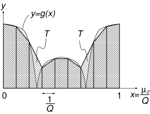
Figure 1: Schematic picture for an expansion of $\sum_{\mu_{2}}|E_{\mu_{1}\mu_{2}}(\Phi)|$ in terms of $1/Q$. This procedure is expressed as eq. (8), and is regarded as an approximation of the curve $y=g(\frac{\mu_{2}}{Q})\equiv|E_{\mu_{1},\mu_{2}}|$ by a collection of segments. Each term in eq. (8) can be associated with an area of a certain region in the figure. The hatched and dotted regions represent the l.h.s. and the first term of the r.h.s. of eq. (8), respectively. Their difference to the order $1/Q^{2}$ (the second term of the r.h.s. of eq. (8)) is represented by narrow arcs between the curve $y=g(x)$ and the segments. There is an additional contribution near the points with $E_{\mu_{1}\mu_{2}}=0$, i.e., from the Fermi level. This comes from the triangular regions, shown as “$T$” in the figure, and results in the $\Phi$-dependent term shown in eq. (9) to the order $1/Q^{2}$.

Next, we consider a two-dimensional cylinder composed of a square lattice [8, 12]. We again consider a nearest-neighbor tight-binding model with the hopping integral $t$. This model can also exhibit the fractional flux periodicity [8, 12]. Let $N$ ($M$) denote the number of lattice sites along (around) the cylindrical axis. The cylinder does not have the twist degree of freedom. The energy eigenvalue of the system is

$$E_{n_{1}n_{2}}(\Phi)=-2t\left\{\cos\left(\frac{n_{1}\pi}{N+1}\right)+\cos\frac{2\pi}{M}\left(n_{2}-\frac{\Phi}{\Phi_{0}}\right)\right\},$$ (15)

where $n_{1}$ and $n_{2}$ are integer quantum numbers and $1\leq n_{1}\leq N$ and $1\leq n_{2}\leq M$. An exact fractional periodicity $\Delta$ of the ground state energy imposes the following equation for any $\Phi$:

$$\sum_{n_{1},n_{2}}\left|\cos\left(\frac{n_{1}\pi}{N+1}\right)+\cos\frac{2\pi}{M}\left(n_{2}-\frac{\Phi}{\Phi_{0}}\right)\right|$$

$$\ =\sum_{n^{\prime}_{1},n^{\prime}_{2}}\left|\cos\left(\frac{n^{\prime}_{1}\pi}{N+1}\right)+\cos\frac{2\pi}{M}\left(n^{\prime}_{2}-\frac{\Phi+\Delta}{\Phi_{0}}\right)\right|.$$

(16)

This requires a transformation between $(n^{\prime}_{1},n^{\prime}_{2})$ and $(n_{1},n_{2})$, which can absorb the fractional flux $\Delta$ in eq. (16). By an analysis similar to that of the twisted torus, we conclude that, for a nontrivial flux periodicity, we should use the re-parameterization $n^{\prime}_{1}=N+1-n_{1}$ and $n^{\prime}_{2}=n_{2}+\frac{M}{2}+\frac{\Delta}{\Phi_{0}}$, which yields a $\frac{\Phi_{0}}{2}$ periodicity for odd $M$.

For an approximate periodicity, only the states near the Fermi level are relevant to the flux-dependent part of the ground state energy to the order $1/M$. In the limits $N\rightarrow\infty$ and $M\rightarrow\infty$ with the fixed integer $Z=2(N+1)/M$, $E_{0}(\Phi)$ has a fractional flux periodicity of $\Delta=\Phi_{0}/Z$ [8, 12] . The ground state energy to the order $1/M$ is given by

$$E_{0}(\Phi)\approx\sum_{n_{1}}\frac{2\pi v_{F}(n_{1})}{Ma}\frac{Q_{L}(n_{1},\Phi)^{2}+Q_{R}(n_{1},\Phi)^{2}}{2}+\text{const.},$$ (17)

where $Q_{L}$ and $Q_{R}$ are defined by eqs. (10) and (11) with $A^{L}(n_{1})=A^{R}(n_{1})\equiv\frac{M}{2}\left(1-\frac{n_{1}}{N+1}\right)$ and the Fermi velocity $v_{F}(n_{1})\equiv 2ta\sin\left(\frac{n_{1}\pi}{N+1}\right)$. When $2(N+1)/M=Z$ is an integer, we can see that the system has a $\Phi_{0}/Z$ periodicity in the $N\rightarrow\infty$ limit. This is similar to that in the case of the twisted torus, and this corresponds to the re-parameterization of quantum numbers of states at the Fermi level: $n^{\prime}_{1}=n_{1}+1$ for $Q_{L}$ and $n^{\prime}_{1}=n_{1}-1$ for $Q_{R}$.

On the basis of the results of the above analyses of the two systems, we can have further insight into the general aspects of fractional flux periodicity. For the exact fractional periodicity $\Delta$, the electron-hole symmetry plays a crucial role; if one breaks the symmetry by shifting the Fermi energy from zero or by allowing a next-nearest-neighbor hopping, the exact fractional periodicity disappears, and only the trivial $\Phi_{0}$ periodicity remains. On the other hand, the approximate periodicity in the limit of a large system is more robust, since it involves only the states near the Fermi level. The approximate fractional flux periodicity is determined from $A^{L}$ and $A^{R}$, which reflects the Fermi wavenumbers. This might be a key to understand experimental results on an approximate fractional flux periodicity in the magnetoresistance of carbon nanotubes [17, 18], for which some theoretical studies [19, 20] have been carried out. A complete explanation of the experimental results is under way.

In summary, we have shown that the fractional flux periodicity is a result of the re-parameterization invariance. This means that if the system has the fractional flux periodicity $\Delta$, the additional fractional flux $\Delta$ can be absorbed by a translation of quantum numbers. For the exact periodicity, it transforms all the states. Meanwhile, for the approximate periodicity, asymptotically valid in large systems, the re-parameterization involves only the states at the Fermi level.

S. M. is supported by a Grant-in-Aid (No. 16740167) from the Ministry of Education, Culture, Sports, Science and Technology, Japan. K. S. is supported by a fellowship of the 21st Century COE Program of the International Center of Research and Education for Materials of Tohoku University. R. S. acknowledges Grants-in-Aid (Nos. 13440091 and 16076201) from the Ministry of Education, Culture, Sports, Science and Technology, Japan.

References

- [1] Y. Aharonov and D. Bohm: Phys. Rev. 115 (1959) 485.
- [2] A. Tonomura, N. Osakabe, T. Matsuda, T. Kawasaki, J. Endo, S. Yano and H. Yamada: Phys. Rev. Lett. 56 (1986) 792.
- [3] M. Büttiker: Phys. Rev. B 32 (1985) 1846.
- [4] H. F. Cheung, Y. Gefen, E. K. Riedel and W. H. Shih: Phys. Rev. B 37 (1988) 6050.
- [5] L. P. Lévy, G. Dolan, J. Dunsmuir and H. Bouchiat: Phys. Rev. Lett. 64 (1990) 2074.
- [6] V. Chandrasekhar, R. A. Webb, M. J. Brady, M. B. Ketchen, W. J. Gallagher and A. Kleinsasser: Phys. Rev. Lett. 67 (1991) 3578.
- [7] D. Mailly, C. Chapelier and A. Benoit: Phys. Rev. Lett. 70 (1993) 2020.
- [8] H. F. Cheung, Y. Gefen and E. K. Riedel: IBM J. Res. Develop. 32 (1988) 359.
- [9] M. Y. Choi and J. Yi: Phys. Rev. B 52 (1995) 13769.
- [10] K. Sasaki, Y. Kawazoe and R. Saito: Phys. Lett. A 329 (2004) 148.
- [11] K. Sasaki, Y. Kawazoe and R. Saito: Prog. Theor. Phys. 111 (2004) 763.
- [12] K. Sasaki, S. Murakami and R. Saito: cond-mat/0407539, to be published in Phys. Rev. B.
- [13] N. Byers and C. N. Yang: Phys. Rev. Lett. 7 (1961) 46.
- [14] It should be mentioned that, for some lattice structures, the Fermi level is not compatible with the conservation of the number of states below the Fermi level when we vary the AB flux. Let us give a simple example. In a one-dimensional tight-binding model with lattice sites, an energy eigenvalue is given by . When we fix the Fermi level as , the number of states below the Fermi level is given by . Therefore, for odd , is not a constant. We can assume that the chemical potential of the system is fixed at to make the system open and applicable to transport experiments.
- [15] N. S. Manton: Ann. Phys. 159 (1985) 220.
- [16] S. Iso and H. Murayama: Prog. Theor. Phys. 84 (1990) 142.
- [17] A. Bachtold, C. Strunk, J. Salvetat, J. Bonard, L. Forro, T. Nussbaumer and C. Schönenberger: Nature 397 (1999) 673.
- [18] A. Fujiwara, K. Tomiyama, H. Suematsu, M. Yumura and K. Uchida: Phys. Rev. B 60 (1999) 13492.
- [19] S. Roche, G. Dresselhaus, M. S. Dresselhaus and R. Saito: Phys. Rev. B 62 (2000) 16092.
- [20] S. Roche and R. Saito: Phys. Rev. Lett. 87 (2001) 246803.