Scaling theory of magneto-resistance in disordered local moment ferromagnets

Abstract

We present a scaling theory of magneto-transport in Anderson-localized disordered ferromagnets. Within our framework a pronounced magnetic-field-sensitive resistance peak emerges naturally for temperatures near the magnetic phase transition. We find that the resistance anomaly is a direct consequence of the change in localization length caused by the magnetic transition. For increasing values of the external magnetic field, the resistance peak is gradually depleted and pushed towards higher temperatures. Our results are in good agreement with magneto-resistance measurements on a variety of disordered magnets.

Complex magnetic materials showing strong magneto-resistance have simultaneously been at the focus of the attention of the magnetic recording industry and the field of strongly correlated electron systems. As a consequence, the interplay between electronic and magnetic degrees of freedom has been intensely studied both experimentally and theoretically during the last four decades.

One of the first theoretical frameworks to provide guidance for understanding magneto-resistance measurements on magnetic metals were provided by de Gennes and Friedel degennes who predicted that long range magnetic fluctuations near the Curie temperature $T_{C}$ will result in a cusp-like singularity of the resistivity $\rho(T)$. As subsequent experiments failed to observe such singular behavior, Fisher and Langer langfish pointed out that $\rho(T)$ shows no anomaly, but it is $d\rho(T)/dT$ that bears resemblance to a cusp near $T_{c}$, and it is caused by short (not long) range magnetic fluctuations.

While the work of Fisher and Langer provided for several decades a very useful theoretical framework to understand magneto-resistance in itinerant magnets, recently discovered complex magnetic materials, such as manganites manganites , and diluted magnetic semiconductors dms do show a resistivity peak directly in $\rho(T)$ and a corresponding anomaly in a relatively large temperature window near $T_{c}$. For magnetic semiconductors and for some of the manganites the before-mentioned resistivity peak appears to be located precisely at $T_{c}$. As pointed out by Littlewood and his coworkers littlewood , such behavior, especially for non-metallic samples, seems to fall outside the range of applicability of the Fisher-Langer model. Several proposals have been made, involving magnetic polarons littlewood , critical spin-flip scattering ohno , thermal magnetic fluctuations within the six-band model brey or Nagaev’s magneto-impurity scattering model nagaev . Most of these theories focus on metallic samples and on producing the resistive anomaly near $T_{C}$, while ignoring non-metallic samples and at least part of the full temperature range.

The available experimental results, however, provide severe constraints if one requires the theoretical framework to reproduce not only the relative shape and position of the anomaly in a narrow temperature window near $T_{C}$ (fluctuation regime), but the actual magnitude of the anomaly, together with the resistive behavior in the paramagnetic and the magnetically ordered phase as well. Furthermore, the theory should explain the fact that, with the application of an external magnetic field, the experimentally observed anomaly is simultaneously reduced in height and pushed towards higher temperatures and the magneto-resistance curves for different external fields never cross. A successful theoretical framework for the magneto-resistance anomaly in disordered magnets should simultaneously satisfy all the experimental constraints mentioned above.

In this paper we show how all properties described above can be explained as a consequence of the interplay between disorder induced localization transition and magnetism, without invoking additional mechanisms such as Jahn-Teller distortion, probably important for some manganites Millis . Our theory is based on simple scaling argument and is relevant for a large number of systems including some of the manganites and a number of magnetic semiconductors.

Let us first discuss how the original one-parameter scaling theory of localization has to be modified to describe magnetic systems. In the standard scaling theory of localization one argues that the typical dimensionless conductance $g(2L)$ of a cube of linear size size $2L$ is uniquely determined by the typical dimensionless conductance $g(L)$ of its pieces of size $L$. This assumption is summarized in the following scaling equation:

$$\frac{d\ln g}{d\ln L}=\beta(g)\;.$$ (1)

The $\beta(g)$ function above depends exclusively on $g$, the dimension, and the symmetry of the Hamiltonian, however, it does not depend on other microscopic properties of the disorder. While $\beta(g)$ can be evaluated for large values of $g$ perturbatively, in order to determine its full shape, numerical computations are needed. For very large $g$, $\beta\approx 1$ in three dimensions, while for very small $g$ it scales as $\beta(g)\approx\ln g$ gangof4 ; localization_review .

The scaling equation above can be used as a powerful tool to analyze the localization transition. Very importantly, in three dimensions the $\beta$ function always vanishes at a critical value $g_{c}$ of $g$, $\beta(g_{c})=0$. This zero of the $\beta$ function is associated with the localization transition: Consider a small piece of mesoscopic size $l_{0}$ having a microscopic conductance $g_{0}$. If $g_{0}>g_{c}$, then the zero temperature dimensionless conductance increases as we increase $L$ and asymptotically behaves as $g(L)\sim\sigma L^{d-1}$, with $\sigma(g_{0})$ the conductivity. For $g<g_{c}$, on the other hand, the conductance scales as $g(L)\sim\exp(-2L/\xi)$, with $\xi(g_{0})$ the localization length. From (1) it follows that for $g_{0}\to g_{c}$ the localization length diverges on the localized side as $\xi\sim(g_{c}-g_{0})^{-\nu}$ while the conductivity goes to 0 on the metallic side of the transition as $\sigma\sim(g_{0}-g_{c})^{\nu}$ in three dimensions. The critical exponent $\nu$ is related to the slope of the beta function at $g_{c}$ as $1/\nu\equiv d\beta/d{\ln}g|_{g_{c}}$.

Let us now consider a disordered local-moment ferromagnet, in which local moments ${\vec{\Omega}}_{i}$ coupled to some charge carriers are responsible for the magnetism. The first observation we make is that - compared to electronic processes - spin fluctuations are usually slow. This is especially true in the vicinity of the ferromagnetic phase transition where the conductance peak of our interest appears. This implies that for transport properties the magnetic moments can be treated as static scatterers, and can be replaced by classical spins $\vec{\Omega}_{i}$. While scattering from these static magnetic moments itself is typically not sufficient to lead to localized charge carriers, it can substantially increase the effect of static disorder, and help to localize charge carriers.

The $T=0$ conductance of a sample of size $L$ will thus depend on the particular distribution of magnetic moments $P(\{\vec{\Omega}_{i}\})$ note . One can argue, however, that the $\beta$ function (1) should depend on this distribution only through the conductance $g_{0}$. Thus the effect of magnetic moments appears in two ways (a) It determines the appropriate symmetry class of the $\beta$ function (Unitary Ensemble = UE), and (b) enters the microscopic conductance $g_{0}=g_{0}(P\{\omega\})=g_{0}[P]$. In general, $g_{0}$ is therefore a complicated non-universal function of temperature, and magnetic field, $g_{0}=g_{0}(T/T_{C},H/T_{C})$ which also depends on the microscopic details of the system. However, once one knows this function and the $\beta$-function, one can use the scaling theory to determine transport properties of the system, as we shall discuss below. One possibility to determine $g_{0}$ is to perform, e.g., a Monte Carlo simulation for a small system, and use the computed conductivity as $g_{0}$.

The scaling equation provides us the conductivity (or localization length) of the electrons, provided that the electronic temperature is zero. In a real system, however, finite temperature has a dual role: On one hand, it changes the distribution $P$ and thus the value of $g_{0}(P)$, but one must also take it into account through the temperature of the conduction electrons. This is a rather complicated task on the metallic side, where the temperature-dependent dephasing length $L_{\rm max}=L_{\varphi}(T)$ provides a cut-off for the scaling, with $L_{\varphi}(T)$ being a non-universal function of the temperature $T$. It is, however, simple to incorporate the effects of finite electronic temperature on the insulating side via Mott’s variable range hopping formula Mott :

$$\sigma\sim{\rm exp}\bigl{\{}-C\bigl{(}\frac{\Delta_{\xi}(P)}{T}\bigr{)}^{1/4}\bigr{\}}\;,$$ (2)

where $\Delta_{\xi}(P)=1/N_{0}\xi^{d}(P)$, with $N_{0}$ the density of states at the Fermi level, and $C$ is a constant of the order of unity foot_note_gap . Note that in this formula $\xi$ must be determined from the integration of the scaling equation, and it therefore depends on $g_{0}(P)$ and thus on the temperature through the distribution $P$.

In order to illustrate the ideas described above, let us consider the disordered Kondo lattice with classical spins:

$$H_{K} = -t\sum_{(i,j),\alpha}c^{\dagger}_{i\alpha}c_{j\alpha}+\sum_{i,\alpha}\epsilon_{i}c^{\dagger}_{i\alpha}c_{i\alpha}$$ (3)

$$+ J\sum_{i,\alpha,\alpha^{\prime}}{\vec{\Omega}}_{i}c^{\dagger}_{i\alpha}{\vec{\sigma}}_{\alpha\alpha^{\prime}}c_{i\alpha^{\prime}}\;.$$

Here $t\equiv 1$ denotes the hopping amplitude of the conduction electrons on a lattice, $c^{\dagger}_{i\alpha}$ creates an electron with spin $\alpha$ at site $i$, and $J$ is the exchange coupling between the spin of the electrons and the classical local moments $\vec{\Omega}_{i}$. The $\epsilon_{i}$-s in Eq. (3) denote random on-site energies, which we generate with a uniform distribution between $\pm W$. In what follows, we shall concentrate on the $J\gg W,t$ limit of Eq. (3), which is relevant for strongly spin-polarized systems such as manganites Millis and some ferromagnetic semiconductors with polarized impurity bands polarized_ferromagn_semic . In this limit Eq. (3) simplifies to:

$$H_{J=\infty}=-\sum_{(i,j)}t_{ij}a^{\dagger}_{i}a_{j}+\sum_{i}\epsilon_{i}a^{\dagger}_{i}a_{i}\;,$$ (4)

where the $a_{i}$ denote spinless Fermions corresponding to the original Fermions aligned antiparallel with the local moments, and $t_{ij}=e^{-i\varphi_{ij}}(1+{\vec{\Omega}_{i}}{\vec{\Omega}_{j}})/2$, with $\varphi_{ij}$ a Berry phase that depends on the directions $\vec{\Omega}_{i}$ and $\vec{\Omega}_{j}$ AndersonHasegawa . The electronic properties of Eq. (4) have been analyzed for completely radom spin orientations in Ref. Bishop . Here, however, we want to study the effect of the ordering of the spins on the electronic properties.

In principle, the finite temperature distribution function of the spins could be computed using an effective action that one obtains by integrating out the conduction electrons at temperature $T$. Instead of doing this, we shall replace this effective action by a simple mean field theory, and assume that the distribution of $\vec{\Omega}_{i}$ is simply given by

$$P_{0}(\vec{\Omega}_{i})\equiv\frac{1}{Z}{\rm exp}[\Omega_{i}^{z}\alpha]\;,$$ (5)

where $\alpha=(H+K\langle\Omega^{z}\rangle)/T]$. Here $H$ denotes an external field, $K$ is an effective exchange coupling between the spins, and the magnetization $m=\langle\Omega^{z}\rangle$ must be determined self-consistently. It is not difficult to see that in this case $P(\vec{\Omega}_{i})$ depends in fact on a single parameter $m\equiv\langle\Omega^{z}\rangle$, which is a universal function of $t=T/T_{C}$ and $h=H/T_{C}$, with $T_{C}=K/3$ being the critical temperature. We computed $m(t,h)$ numerically by solving simple transcendental equations.

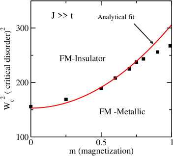
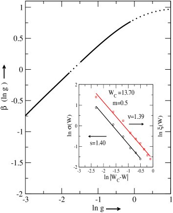
Figure 1: Top: Zero temperature localization phase diagram of the Kondo lattice model defined in the text obtained from a finite size scaling analysis of Ljapunov exponents (dots). The localization phase transition is shifted towards stronger disorder as we align the spins. The dashed line denotes the phase boundary obtained using the naive estimate, Eq. (6). Bottom: Beta function obtained numerically from the scaling analysis. The inset shows the divergence of the localization length and the resistivity at the critical disorder for the case $m=0$. We estimate the critical exponent to be $\nu\approx 1.4$.

To obtain the phase diagram of the model defined by Eqs. (4) and (5) we carried out a careful transfer matrix analysis within the formalism following the original work of McKinnon and Kramer KramersMcKinnon ; Pascu . The main results of our analysis are summarized in Fig. 1 for a carrier concentration 0.5 electron/spin. Firstly, we find that larger and larger disorder is needed to obtain a localized phase for increasing $m$ (see the phase boundary in Fig.1a). In other words, aligning spins delocalizes electrons, and leads to a decrease of the resistivity. We performed a scaling analysis of the Ljapunov exponents and found that for $m<0.9$ all data collapsed to a single scaling curve, independent of the specific value of $m$, confirming the single parameter scaling hypothesis made earlier. Note, however, that the $m\approx 1$ data could not be collapsed with the $m<1$ data. This is quite natural, since for $m=1$ the Hamiltonian belongs to a different symmetry class (Orthogonal Ensemble). The scaling analysis also made us possible to estimate the $\beta$ function shown in Fig. 1b. The critical exponent $\nu\approx 1.4$ is in good agreement with the earlier results of Ref. Ohtsuki for the unitary ensamble.

The phase boundary can be qualitatively understood if we assume that the microscopic conductance is proportional to the conductance of a single bond. In the most naive approximations, the effect of the magnetic field is just to reduce the effective value of the hopping, $t^{2}\to t_{\rm eff}^{2}=t^{2}f(m)$, and the conductance is roughly proportional to $\sim t_{\rm eff}^{2}/W^{2}$,

$$g_{0}(m)\approx C{t_{\rm eff}^{2}\over W^{2}}={\tilde{g}}_{0}\;f(m)\;,$$ (6)

where $\tilde{g}_{0}=g_{0}(m=1)$ denotes the microscopic conductance for fully aligned spins. The function $f(m)=f(m(h,t))$ can be obtained in this approximation from the phase boundary, which is determined by the condition $g_{0}(m)=g_{c}$, and is simply given by $W_{c}(m)=W_{c}(m=1)\sqrt{f(m)}$. As shown in Fig. 1a, the simple function $f(m)=(1+m^{2})/2$ gives a very reasonable agreement with the numerical phase boundary.

Having $f(m)$ and the $\beta$-function at hand, we can now carry out the program outlined above and combine Eqs. (1), (2), and (6) to determine the temperature-dependence of the conductivity in the localized phase. For the sake of simplicity, we shall assume that we are close enough to the metal-insulator transition, and approximate the $\beta$-function as $\beta(g)\approx\frac{1}{\nu}\ln(g/g_{c})$ with $\nu\approx 1.4$. Since $\nu$ is not far from 1, this is a reasonable approximation. In this case the resistivity can be expressed as

$${\rm ln}\varrho=A\left[{\rm ln}\frac{g_{c}}{g_{0}(m)}\right]^{3\nu/4}\frac{1}{t^{1/4}};,$$ (7)

where $A$ is a constant of the order of unity, and $g_{c}/g_{0}(m)=B/f(m(t,h))$. The constant $B$ here measures simply the distance from the localized phase, $B=g_{c}/g_{0}(m=1)$, and $f(m)$ is the scaling function in Eq. (6).

Typical results are summarized in Fig. 2 for $B=1.5$ and $B=4$. The resistivity curves are strikingly similar to the ones measured in various compounds in or in the vicinity of the localized phase, and clearly display a large peak at $T_{C}$ and a giant negative magneto-resistance manganites ; Millis . This peak is simply a consequence of reducing the localization length while entering the magnetic phase, and has nothing to do with critical fluctuations (which may also lead to additional contributions Felix ). The magnetic field dependence of the data also agrees qualitatively with the one seen in the experiments: The peak is getting flat and shifts upward with increasing magnetic field. One of the most important properties of the experimental data is that the resistivity curves corresponding to different magnetization do not cross. The theory of Ref. nagaev , e.g. does not seem to satisfy this criterion gurin , while in our theory, this is a natural consequence of the reduction of $\xi$. Note that in the absence of localization effects / disorder, the resistivity would not display a peak at $T_{c}$ brey ; furukawa . We find a similar peak structure in the metallic phase, however, there the precise shape of the anomaly depends also on the assumption made for the temperature dependence of the dephasing length, $L_{\varphi}(T)$.

In conclusion, in the present paper we have studied the interplay of disorder and magnetization in disordered local moment ferromagnets. We proposed a unified framework to study the localization phase transition in these materials and argued that a unique beta function can be used to describe the localization phase transition in these materials. We verified the above hypothesis for a simple model of disordered local moment ferromagnets. The scaling approach of this paper allowed us to estimate the temperature and magnetic field dependence of the resistivity in the localized phase of the mean field model studied. The obtained resistivity curves display a peak in the resistivity at the critical point, due to the interplay of magnetism and disorder. This resistivity maximum is gradually suppressed and shifted towards higher temperatures upon application of a magnetic field, and the computed resistivity curves do not cross. Our simple theory thus seems to explain all basic features of the resistivity anomalies observed in many feromagnetic semiconductors in the ’localized’ phase and some of the manganites.

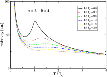
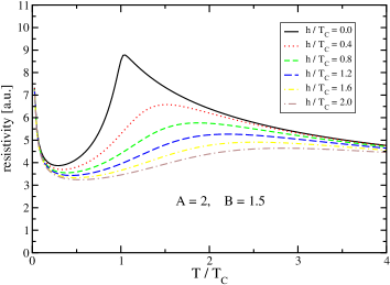
Figure 2: Resistivity computed from Eq. (7) for the localized phase of the mean field model discussed in the text. We used $A=2$ and $\nu=1.4$ for the curves presented. The top figure shows the resistivity for parameters not very far from the localization phase transition ($B=1.5$), while the bottom figure displays resistivity curves computed deep in the localized phase ($B=4$). A peak appears at $T_{c}$ due to the interplay of magnetic ordering and localization, and is shifted to higher temperatures upon application of magnetic field.

We would like to thank J.K. Furdyna, P. Schiffer, I. Varga, T. Wojtowicz, and especially Peter Littlewood for valuable discussions. We would also like to thank P. Schiffer and B.-L. Sheu for sharing their results prior to publication. This research has been supported by NSF-MTA-OTKA Grant No. INT-0130446, Hungarian Grants No. OTKA T038162, T046267, and T046303, and the European ’Spintronics’ RTN HPRN-CT-2002-00302. B.J. was supported by NSF-NIRT award DMR02-10519 and by the Alfred P. Sloan Foundation.

References

- (1) P.G. de Gennes and J. Friedel, J. Phys. Chem. Solids 4, 71 (1958).
- (2) M.E. Fisher and J.S. Langer, Phys. Rev. Lett., 20 665 (1968).
- (3) G. Matsumoto, J. Phys. Soc. Jpn. 29, 613 (1970); S. Jin, T. H. Tiefel, M. McCormack, R. A. Fastnacht, R. Ramesh, and L. H. Chen, Science 264, 413 (1994); W. Boujelben et al., Physica B 321, 68 (2002).
- (4) See, for example F. Matsukura et al. Phys. Rev. B 57, R2037 (1998).
- (5) P. Majumdar and P. B. Littlewood, Nature 395 479 (1998); P.B. Littlewood, Acta Phys. Pol. 97, 7 (2000).
- (6) T. Omiya et al.m Physica E (Amsterdam) 7, 976 (2000).
- (7) M. P. Lopez-Sancho and L. Brey, Phys. Rev. B 68, 113201 (2003).
- (8) E. L. Nagaev, Phys. Rep. 346, 387 (2001).
- (9) P. Gurin (unpublished).
- (10) This distribution of spins depends, of course, on the temperature considered.
- (11) E. Abrahams, et al., Phys. Rev. Lett. 42, 673 (1979).
- (12) For a review on localization theory, see e.g., P. A. Lee and T. V. Ramakrishnan, Rev. Mod. Phys. 57, 287 (1985).
- (13) A. MacKinnon and B. Kramer Phys. Rev. Lett. 47, 1546 (1981).
- (14) In general, electron-electron interaction induces a Coulomb gap in the density of sattes of the quasiparticles [Efros, A. L., and B. I. Shklovskii, J. Phys. C 8, L49 (1975)]. Here we assume that we are close to the localization transition and therefore this pseudogap is negligeable at the energy scales considered. Under these conditions Mott’s variable range formula for non-interacting electrons can be used.
- (15) P. W. Anderson and H. Hasegawa, Phys. Rev. 100, 675 (1955).
- (16) Q.Li et al., Phys. Rev. B 56, 4541 (1997).
- (17) Though the experimental situation is unclear, some theoretical works propose that holes are spin-polarized even in metallic dilute magnetic semiconductors. See e.g. J. Schliemann, J. König, and A.H. MacDonald, Phys. Rev. B 64, 165201 (2001); A. Chattopadhyay, S. Das Sarma, and A.J. Millis, Phys. Rev. Lett. 87, 227202 (2001).
- (18) C.P. Moca, G. Zaránd, and B. Jankó, (unpublished).
- (19) K. Slevin and T. Ohtsuki, Phys. Rev. Lett. 82, 382 (1999).
- (20) N.F. Mott, J. Non-Cryst. Solids 1, 1 (1968).
- (21) C. Timm et al., (unpublished); C. Timm, M.E. Raikh, F. von Oppen, cond-mat/0408602.
- (22) A. J. Millis, B. I. Shraiman, and R. Mueller, Phys. Rev. Lett. 77, 175 (1996).
- (23) N. Furukawa, J. Phys. Soc. Jpn. 64 3164 (1995), [cond-mat/9505117].