Singular conductance of a spin 1 quantum dot

Abstract

We interpret the recent observation of a zero-bias anomaly in spin-1 quantum dots in terms of an underscreened Kondo effect. Although a spin-1 quantum dots are expected to undergo a two-stage quenching effect, in practice the log normal distribution of Kondo temperatures leads to a broad temperature region dominated by underscreened Kondo physics. General arguments, based on the asymptotic decoupling between the partially screened moment and the leads, predict a singular temperature and voltage dependence of the conductance $G$ and differential conductance $g$, resulting in $dg/dT\sim 1/T$ and $dG/dV\sim 1/V$. Using a Schwinger boson approach, we show how these qualitative expectations are borne out in a detailed many body calculation.

Single-electron transistors (SETs) offer the intriguing opportunity to probe and explore classes of strongly correlated electron behavior associated with the Kondo effect that are difficult to access in bulk materialsphysicsworld ; raikh ; lee ; ggordon ; koevenhoven . The possibility of observing a break-down in Landau Fermi liquid behavior that accompanies the overscreened two-channel Kondo effect in quantum dots has been a subject of particular recent interesttwochannel1 ; twochannel2 . In this paper, we propose that singular deviations from Landau Fermi liquid behavior associated with the underscreened Kondo effect, hitherto unobserved in bulk materials, will develop in conventional quantum dots with even numbers of electrons and a triplet ground-stateschmid ; sasaki ; kogan . These deviations from conventional Fermi liquid behavior are predicted to lead to singular voltage, field and temperature dependences in the conductance.

The Kondo effect in quantum dots with odd numbers of electrons, predicted more than fifteen years ago, raikh ; lee is now well-established by experiment ggordon ; koevenhoven . Subsequent observations have shown that zero-bias anomalies associated with a Kondo effect can also occur in quantum dots with even occupancies, where Hund’s coupling between the electrons can lead to novel degeneracies, through the formation of higher spin states, or the accidental degeneracy of singlet and triplet states. Zero-bias anomalies in integer spin quantum dots were first reported by Schmid et al.schmid . Sasaki et alsasaki later discovered a zero-bias anomaly in even electron quantum dots, associated with the degeneracy point between singlet and triplet states, tuned by a small magnetic field. Most recently, Kogan et alkogan have shown that the singlet-triplet excitation energy in lateral quantum dots can be tuned by the gate voltage, explicitly demonstrating that the zero bias anomaly develops once the triplet state drops below the singlet configuration.

Pustilnik and Glazmanpustilnik have analyzed the low-temperature Fermi liquid physics of higher spin quantum dots. Their analysis shows that lateral quantum dot in a triplet configuration develops two screening channels which fully screen the local moment at the lowest temperatures. Using the Landauer formula, they deduce the conductance $G$ of the Fermi liquid which develops to be

$$G=\frac{2e^{2}}{h}\sin^{2}(\delta_{1}-\delta_{2})$$ (1)

where $\delta_{1}$ and $\delta_{2}$ are the scattering phase shifts of the two screening channels. According to this line of reasoning, the development of a unitary phase shift in each channel, $\delta_{1}=\delta_{2}=\pi/2$ leads to a complete suppression of the zero bias anomaly in a triplet quantum dotzarand . Why then, are zero-bias anomalies, with near unitary conductance seen in triplet quantum dots?

In this paper we propose an interpretation of this unexpected behavior in terms of an underscreened Kondo effect. Our key observation is that the antiferromagnetic Kondo coupling constants $J_{\lambda}$ ($\lambda=1,2$) associated with the two screening channels in a triplet quantum dot will generally be distributed independently. Since the Kondo temperature depends exponentially on the coupling constant $T_{K\lambda}=D\sqrt{J_{\lambda}\rho}e^{-\frac{1}{J_{\lambda}\rho}}$, a normal distribution of the coupling constants will drive a log-normal distribution in the two Kondo temperatures lognormal , with the potential to generate exponentially large separations in the relative magnitude of the Kondo temperatures of each channel. If we assume that $\ln(T_{K1}/T_{K2})=\frac{1}{J_{2}\rho}-\frac{1}{J_{1}\rho}>>1$, then over the exponentially broad temperature range given by $\log(T_{K1})>>\log T>>\log(T_{K2})$, the underlying physics is that of a one channel spin-1 Kondo model, in which the spin is partially screened to a spin 1/2.

From this perspective, triplet dots with a large zero bias anomaly are those where the Kondo coupling constants of the two channels are severely mis-matched, giving rise to decades of behavior dominated by the under-screened Kondo effect in a single channel. Previous work, both analyticpustilnik and numerical hofstetter2 ; zarand has focussed on the equilibrium behavior of triplet quantum dots with Kondo temperatures of comparable magnitude. We now examine the singular consequences of a wide separation between these two scales in both finite temperature and finite voltage properties.

In the underscreened spin-1 Kondo effect, the residual spin-1/2 moment is ferromagnetically coupled to leads, with a coupling that scales logarithmically slowly to zeronozieres . The ground-state which develops is a “singular Fermi liquid”, in which the electrons do behave as Landau quasiparticles which are elastically scattered with unitary phase shift, but where, on the other hand, a logarithmically decaying coupling generates a singular energy dependence in the scattering phase shift and a divergence in the resulting quasiparticle density of statespepin ; pankaj ; indranil . The Hamiltonian for the underscreened quantum dot is

$$H = H_{0}+J\psi^{\dagger}_{\alpha}\vec{\sigma}_{\alpha\beta}\psi_{\beta}\cdot\vec{S},$$

$$H_{0} = \sum_{k,\lambda=R,L,\sigma}\epsilon_{k}c^{\dagger}_{k\lambda\sigma}c_{k\lambda\sigma}$$ (2)

where $\psi_{\sigma}=\sum_{k}\alpha c_{kL\sigma}+\beta c_{kR\sigma}$ denotes the linear combination of right and left channels that couples to the dominant screening channel. Much is known about the equilibrium physics of this model. At low temperatures, the spin is partially screened from spin $S$ to spin $S-(1/2)$. The residual moment is ferromagnetically coupled to the conduction sea, with a residual coupling that slowly flows to weak coupling according to

$$J\rho(\Lambda)=-\frac{1}{\ln(\frac{T_{K}}{\Lambda})}+O\left(\frac{1}{\ln^{2}(\frac{T_{K}}{\Lambda})}\right)$$ (3)

where $\Lambda\sim max(T,\mu_{B}B)$ is the characteristic cut-off energy scale, provided in equilibrium, by the temperature or magnetic field. At low energies and temperatures, the partially screened magnetic moment scatters electrons elastically, with a unitary phase shift, however the coupling to the residual spin $(S-\frac{1}{2})$ gives rise to a singular energy dependence of the scattering phase shift. The low energy scattering phase shift can be directly deduced from the Bethe Ansatz, and has the asymptotic form

$$\delta(\omega)=\frac{\pi}{2}-\pi\rho J(\omega)=\frac{\pi}{2}\left(1+\frac{(S-\frac{1}{2})}{\ln(T_{K}/\omega)}\right).$$ (4)

The logarithmic term on the right hand side is produced by the residual coupling between the electrons and the partially screened moment. While the electrons at the Fermi energy scatter elastically off the local moment with unitary scattering phase shift, as in a Fermi liquid, the logarithmically singular dependence of the phase shift leads to a divergent density of states, $N(\omega)\sim\frac{1}{\pi}\frac{d\delta(\omega)}{d\omega}\sim\frac{1}{|\omega|}$, which means that we can not associate this state with a bona-fide Landau Fermi liquid. For this reason, the ground-state of the underscreened Kondo model has recently been called a “singular Fermi liquid”pankaj .

These singular features of the underscreened Kondo effect are expected to manifest themselves in the properties of the triplet quantum dot. For example, we expect the low-field conductance to follow the simple relation

$$G(B)=\frac{2e^{2}}{h}\sin^{2}\delta(B)\sim\frac{2e^{2}}{h}\left(1-\frac{\pi^{2}}{16}\frac{1}{ln^{2}\left(\frac{T_{K}}{\tilde{B}}\right)}\right),$$ (5)

for $\tilde{B}<<T_{K}$. This relationship was previously obtained by other means from the $T_{K2}\rightarrow 0$ of the two-channel modelpustilnik . Notice that the field derivative of the conductance diverges as $\frac{dG}{dB}\propto 1/\left(Bln^{3}({T_{K}}/{\tilde{B}})\right)$ at low fields. The prediction of the finite temperature, and finite voltage conductance can not be made exactly, however we expect the above form to hold, for the differential conductance at finite temperature or voltage, with an appropriate replacement of cut-offs, namely

$$G(V,T)\sim\frac{e^{2}}{h}\left(1-\frac{\pi^{2}}{16}\frac{1}{ln^{2}\left(\frac{T_{K}}{{\rm max}(T,eV)}\right)}\right)$$ (6)

and $dG/dT\sim 1/max(T,V)$.

To model this behavior in more detail it is useful to consider a simplified model of the quantum dot in which the Hund’s coupling is taken to be infinite. In this limit, the states of the quantum dot can be described using a Schwinger boson representation as

$$|d^{1},\sigma\rangle=b^{\dagger}_{\sigma}\chi^{\dagger}|0\rangle,\qquad\qquad|d^{2},M\rangle=b^{\dagger}_{\sigma}b^{\dagger}_{M-\sigma}|0\rangle,$$ (7)

Written in this representation the model becomes

$$H=H_{0}+t\sum_{\sigma}\left[\psi^{\dagger}_{\sigma}\chi^{\dagger}b_{\sigma}+b_{\sigma}^{\dagger}\chi\psi_{\sigma}\right]+E_{d}\chi^{\dagger}\chi$$ (8)

subject to the constraint $n_{b}+\chi^{\dagger}\chi=2$.

To develop a controlled many body treatment of this Hamiltonian, we use a large-$N$ expansion, extending the number of spin components $\sigma$ from two to $N$. To preserve a finite scattering phase shift as $N\rightarrow\infty$, we introduce $K=kN$ bosonic “replicas”, where $k$ is fixed. With this device we obtain a (dynamical) mean field theory with scattering phase shift $\delta=\pi k$ and the qualitatively correct logarithmic energy dependences indranil . The Hamiltonian used in the large $N$ expansion is then

$$H=H_{0}+\frac{\tilde{t}}{\sqrt{N}}\sum_{\sigma,\mu}\left[\psi^{\dagger}_{\sigma}\chi_{\mu}^{\dagger}b_{\sigma}+b_{\sigma}^{\dagger}\chi\psi_{\sigma}\right]+E_{d}\sum_{\mu=1}^{kN}\chi_{\mu}^{\dagger}\chi_{\mu}.$$ (9)

In the large N limit, there are two self-consistent non-crossing approximations to the Dyson equations for the self-energies of the conduction electrons and $\chi$ fermions (Fig. 1). Here we sketch the main elements of the derivation. As in the corresponding equilibrium calculationindranil , the boson behaves as a sharp excitation in the large $N$ limit, with an average occupancy $\langle n_{b\sigma\mu}\rangle=n_{b}/N$. From the Dyson equations we obtain sets of self-consistent integral equations for both the retarded and Keldysh self-energies. The explicit expressions for the the retarded self-energies $\Sigma^{\chi}_{R}$ and $\Sigma^{c}_{R}$ of the slave fermion ($\chi$) and the conduction electrons ($c$) are

$$\Sigma^{\chi}_{R}(\omega) = -{\tilde{t}}^{2}n_{b}G_{A}(\lambda-\omega)-{\tilde{t}}^{2}\int\frac{d\omega^{\prime}}{\pi}f_{c}(\omega^{\prime})\frac{1}{\omega^{\prime}+\omega-\lambda+i\delta}ImG_{R}(\omega^{\prime}),$$ (10)

$$\Sigma^{c}_{R}(\omega) = -{\tilde{t}}^{2}kn_{b}J_{A}(\lambda-\omega)-{\tilde{t}}^{2}k\int\frac{d\omega^{\prime}}{\pi}f_{\chi}(\omega^{\prime})\frac{1}{\omega^{\prime}+\omega-\lambda+i\delta}ImJ_{R}(\omega^{\prime}).$$ (11)

Here $J_{R}(\omega)=[\omega-E_{d}-\Sigma^{\chi}_{R}(\omega)]^{-1}$ and $G_{R}^{c}(\omega)=[(-\pi\rho)^{-1}-\Sigma_{R}^{c}(\omega)]^{-1}$ are the retarded propagators for the $\chi$ fermions and conduction electrons.

Figure 1: The non-crossing approximation for the self-energies of conduction electrons and $\chi$ fermions. The solid line denotes the Larkin Ovchinnikov matrix propagator for the conduction electrons. The dashed line denotes the corresponding Green’s function of the auxiliary ($\chi$) fermions and the wavy line is the bosonic propagator. Thin lines denote the bare propagator and full lines the dressed propagator. Each vertex corresponds to the factor $\frac{\tilde{t}}{\sqrt{N}}$.

The ratio of the Keldysh to the retarded self-energies self-consistently determines the fermion distribution functions. We can summarize the results of our calculation of the Keldysh self-energies by providing the distribution functions that they generate. The distribution function of the conduction electrons is the average

$$f_{c}=\frac{1}{2}\left[f_{L}(\omega)+f_{R}(\omega)\right],$$ (12)

where $f_{L,R}(\omega)=1/(e^{\beta(\omega\mp eV/2}+1)$ is the equilibrium distribution function in the left/right-hand lead. The distribution function of the auxiliary fermion is

$$f_{\chi}(\omega)=\frac{n_{b}[1-f_{c}(\omega)]}{n_{b}+f_{c}(\omega)},$$ (13)

where $n_{b}=1/(e^{\beta\lambda}+1)$ determines $\lambda$. This relationship can be simply understood as the result of detailed balance between rate of the decay processes $c\rightarrow b+\chi$ and $b+\chi\rightarrow c$, and it reverts to the equilibrium Fermi Dirac distribution in the limit $V\rightarrow 0$.

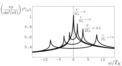
Figure 2: Imaginary part of dot T-matrix for a variety of voltages for the case $k=0.4$. As the voltage is increased, the singular central peak splits into two components.

From these results, we compute the temperature and voltage dependent current, given by wingreenmeir

$$I(V,T)=N\frac{e^{2}V}{h}\rho\int{d\omega}\frac{[f_{L}(\omega)-f_{R}(\omega)]}{eV}{\rm Im}t_{R}(\omega)$$ (14)

where $t_{R}(\omega)=\Sigma^{c}_{R}(\omega)/[1-i\pi\rho\Sigma^{c}_{R}(\omega)]$ is the scattering t-matrix.

We have solved these equations numerically, and the key results are shown in Figs 2-4. Fig. 2. shows the voltage dependent t-matrix at zero temperature. At zero voltage, the t-matrix contains a logarithmic singularity noted in previous workhofstetter2 ; indranil which splits into two peaks at a finite voltage. In our calculation, the split Kondo resonance retains its singular structure, although this is most likely an artifact of taking a limit where the bosons behave as a sharp excitation. In Fig. 3., we show the temperature dependent conductance.

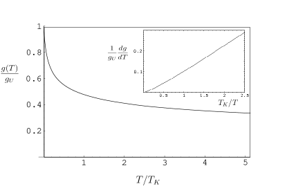
Figure 3: Temperature dependence of the differential conductance, normalized with respect to $g_{U}=N\frac{e^{2}}{h}sin^{2}(\pi k)$ for the representative case $k=0.4$. Insert shows the $1/T$ divergence of the derivative $dg/dT$.

The temperature-dependent deviations from unitary conductance are determined by the logarithmic singularity in the phase shift, and in our calculation, these are proportional to $1/\ln(T_{K}/{\rm max}(eV,T))$. In the Schwinger boson approach, the number of bound bosons in the Kondo singlet never exceeds $N/2$ and the region $K\geq N/2$ does not describe an underscreened Kondo model. Consequently, we are limited to static phase shifts $\delta=\pi(K/N)<\pi/2$, so the strictly particle-hole symmetric case $\delta=\pi/2$ is outside the limits of our approach. Nevertheless, our numerical results do capture the expected singularities. Fig. 3. shows the singular form of the temperature dependent conductance, with singular $1/T$ divergence in $dg/dT$.

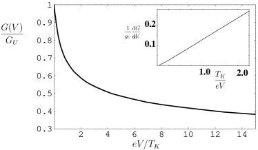
Figure 4: Voltage dependent conductance $G(V)=I(V)/V$ for the case $k=0.4$. Insert: $dG(V)/dV$ showing $1/V$ divergence.

Finally, Fig. 4. shows the voltage dependence of the conductance, which has a similar logarithmic singularity at low voltage.

In summary, we have proposed that the monotonically increasing conductance observed as the temperature is lowered in triplet quantum dots is associated with an underscreened Kondo effect. The singular energy and temperature dependence associated with the Kondo resonance is predicted to give rise to a $1/T$ divergence in the temperature dependence of the differential conductance, and a $1/V$ divergence in the second derivative of the voltage dependent current $d^{2}I/dV^{2}$. These ideas have been developed qualitatively and illustrated within an integral equation treatment of the underscreened Kondo model. Experimental observation of these singular features would constitute a first realization of the underscreened Kondo effect.

The authors wish to thank H. Kroha, G. Zarand and M. Eschrig for discussions related to this work. This research was partly supported by the Alexander Von Humboldt foundation (AP) and DOE grant DE-FG02-00ER45790 (PC).

References

- (1) Leo Kouwenhoven and Leonid Glazman, Physics World 14, 33 (2001).
- (2) L. I. Glazman and M. E. Raikh, JETP Lett. 47, 452 (1988).
- (3) T. K. Ng and P. A. Lee, Phys. Rev. Lett. 61, 1768 (1988).
- (4) D. Goldhaber-Gordon, Hadas Shtrikman, D. Mahalu, David Abusch-Magder, U. Meirav and M. A. Kastner, Nature 391, 156 (1998)
- (5) S.M. Cronenwett et al., Science, 281, 540 (1998).
- (6) Yuval Oreg, David Goldhaber-Gordon, Phys. Rev. Lett. 90, 136602 (2003).
- (7) M.G. Vavilov, L.I. Glazman, cond-mat/0404366 , (2004).
- (8) J. Schmid, J. Weis, K. Eberl, and K. v. Klitzing, Phys. Rev. Lett. 84, 5824 (2000).
- (9) S. Sasaki, S. De Franceschi, J. M. Elzerman, W. G. van der Wiel, M. Eto, S. Tarucha and L. P. Kouwenhoven, Nature 405, 764 (2000).
- (10) A. Kogan, G. Granger, M. A. Kastner, D. Goldhaber-Gordon, H. Shtrikman, Phys. Rev. B 67, 113309 (2003).
- (11) M. Pustilnik and L. I. Glazman, Phys. Rev. Lett. 87, 216601 (2001).
- (12) W. Hofstetter, G. Zarand, Phys. Rev. B 69, 235301 (2004).
- (13) O. O. Bernal, D. E. MacLaughlin, H. G. Lukefahr, B. Andraka, Phys. Rev. Lett. 75, 2023 (1995); R. N. Bhatt and D. S. Fisher, Phys. Rev. Lett. 68, 3072, 1992; V. Dobrosavljevic, T. R. Kirkpatrick and G. Kotliar, Phys. Rev. Lett. 69, 1113 (1992).
- (14) W. Hofstetter & Herbert Schoeller, Phys. Rev. Lett. 88, 016803 (2002)
- (15) P. Nozières, Journal de Physique C 37, C1-271, 1976 ; P. Nozières and A. Blandin, Journal de Physique 41, 193, 1980.
- (16) P. Coleman and C. Pepin, Phys. Rev. B 68, 220405(R) (2003).
- (17) Pankaj Mehta, L. Borda, G.Zarand, N. Andrei, P. Coleman, cond-mat/0404122 (2004).
- (18) I. Paul and P. Coleman, cond-mat/0404001 (2004).
- (19) Y. Meir and N. S. Wingreen, Phys. Rev. Lett. 68, 2512 (1992).