The Initial Configuration of Young Stellar Clusters: A $K$–band Number Counts Analysis of the Surface Density of Stars

Abstract

We present an analysis of stellar distributions for the young stellar clusters GGD 12-15, IRAS 20050+2720, and NGC 7129, which range in far-IR luminosity from 227 to 5.68 $\times 10^{3}~{}L_{\odot}$ and are all still associated with their natal molecular clouds. The data used for this analysis includes near-IR data obtained with FLAMINGOS on the MMT Telescope and newly obtained wide-field 850 $\mu$m emission maps from SCUBA on the JCMT. Cluster size and azimuthal asymmetry are measured via azimuthal and radial averaging methods respectively. To quantify the deviation of the distribution of stars from circular symmetry, we define an azimuthal asymmetry parameter and we investigate the statistical properties of this parameter through Monte Carlo simulations. The distribution of young stars is compared to the morphology of the molecular gas using stellar surface density maps and the 850 $\mu$m maps. We find that two of the clusters are not azimuthally symmetric and show a high degree of structure. The GGD 12-15 cluster is elongated, and is aligned with newly detected filamentary structure at 850 $\mu$m. IRAS 20050+2720 is composed of a chain of three subclusters, in agreement with Chen et al. (1997), although our results show that two of the subclusters appear to overlap. Significant 850 $\mu$m emission is detected toward two of the subclusters, but is not detected toward the central subcluster, suggesting that the dense gas may already be cleared there. In contrast to these two highly embedded subclusters, we find an anti-correlation of the stars and dust in NGC 7129, indicating that much of the parental gas and dust has been dispersed. The NGC 7129 cluster exhibits a higher degree of azimuthal symmetry, a lower stellar surface density, and a larger size than the other two clusters, suggesting that the cluster may be dynamically expanding following the recent dispersal of natal molecular gas. These analyses are further evidence that embedded, forming clusters are often not spherically symmetric structures, but can be elongated and clumpy, and that these morphologies may reflect the initial structure of the dense molecular gas. Furthermore, this work suggests that gas expulsion by stellar feedback results in significant dynamical evolution within the first 3 Myr of cluster evolution. We estimate peak stellar volume densities and discuss the impact of these densities on the evolution of circumstellar disks and protostellar envelopes.

1. Introduction

It is now commonly accepted that most stars form in clusters of 100 or more stars (Lada & Lada, 2003; Porras et al., 2003; Carpenter, 2000). In addition, young OB stars nearly always appear in groups and clusters of lower mass stars (Testi, Palla, & Natta, 1999; Megeath et al., 2002). Clearly, understanding the process of forming stars in clusters is of considerable importance. Although we have an increasingly detailed picture of relatively isolated star formation in nearby dark clouds such as those in the Taurus complex, our understanding of formation in clusters has been hindered by greater observational and theoretical challenges.

Observationally, the challenges of studying embedded clusters are their distance, their spatial density, and their association with high column density molecular clouds. While the Taurus complex provides a number of examples of isolated star formation at 160 pc, most clusters are at distances of 300 pc or greater (Lada & Lada, 2003; Porras et al., 2003), and thus require greater angular resolution and sensitivity to study. The stars in these regions may be closely spaced, again requiring high angular resolution to resolve the individual stars. Finally, many clusters are deeply embedded, and are thus obscured to observation at visible wavelengths. For this reason, the importance of young stellar clusters was not realized until infrared cameras with detector arrays became available (Lada, 1992). With the latest generation of wide field cameras on 6-10 meter class telescopes, near-IR observations can now probe a large sample of young clusters with the sensitivity to detect objects well below the hydrogen burning limit, the angular resolution to resolve high density groupings of stars, and the field of view necessary to observe the distribution of stars over multi-parsec distances. Furthermore, the Spitzer Space Telescope is now providing detailed images of young clusters in the mid-IR, allowing us for the first time to identify young stars with disks and infalling envelopes efficiently in clusters out to 1 kpc and beyond (e.g., Megeath et al., 2004; Whitney et al., 2004).

Theoretically, the problem of star formation in clusters is perhaps an even greater challenge, as a realistic analysis must include a network of non-linear processes, such as turbulent motions and shocks in the natal molecular cloud, potential collisions and multi-body interactions between young stars and protostars, and the destructive influence of radiation and winds from the newly formed stars. Numerical models of turbulent fragmentation have been successful at simulating the formation of clusters (or at least clusters of protostellar gravitationally bound cores) and these simulations are beginning to yield a wealth of theoretical predictions which can now be investigated observationally (e.g., Klessen & Burkett, 2000; Klessen, Heitsch, & Mac Low, 2000; Bate, Bonnell, & Bromm, 2003; Bonnell, Bate, & Vine, 2003; Gammie et al., 2003; Li et al., 2004). For example, numerical simulations by Bate, Bonnell, & Bromm (2003) and Bonnell, Bate, & Vine (2003) of turbulent, initially spherically symmetric, Jeans unstable molecular clouds produce collapsing, non-uniform filamentary density structures which are formed through the dissipation of kinetic energy by hydrodynamic shocks, allowing gravity to overcome turbulent support and force collapse. In these simulations, the gas eventually fragments into small ($<200$ AU), self-gravitating, sub-virial clumps, which are interpreted as protostars. The models produce multiple groups of protostars which eventually merge to form large clusters. However, these simulations have obvious limitations: there are numerical problems associated with following the collapse of gas from parsec to 100 AU size scales, the models assume idealized initial conditions, and the models also do not take into account the feedback from the newly formed stars. In particular, the later stages of the evolution in these models may have questionable relevance to real clusters given that most young stellar clusters do not evolve into bound clusters, in part due to the dispersal of most of the binding mass before it forms stars (Lada & Lada, 2003).

With increasingly sophisticated numerical models beginning to predict the spatial distribution and densities of young stars, it is an appropriate time to explore the configuration of young stellar clusters through wide-field infrared and submillimeter imaging, both to test current models and to guide the development of future models. Through the analysis of the stellar surface density in young ($<3$ Myr) stellar clusters still associated with their natal molecular gas, and through a comparison of the corresponding dust and gas density structure, we can study the initial configuration of young clusters and their subsequent dynamical evolution. We are now engaged in a multi-wavelength study of the structure of young stellar clusters, including ground-based near-IR data, Spitzer mid-IR imaging, and ground-based submillimeter and millimeter-wave imaging (Gutermuth et al., 2004; Megeath et al., 2004). While testing cluster formation models is a long-term goal of the project, this paper is primarily focused on developing quantitative techniques for analyzing the spatial structure of young stellar clusters and applying these techniques to new observations of three clusters. Subsequent papers will apply these techniques to the full sample of clusters observed in our survey. It is our hope that this work will encourage modelers to provide more accessible observable quantities from their simulations.

In this paper, we present an initial analysis of near-IR and submillimeter imaging of three clusters using near-IR images from FLAMINGOS on the 6.5 meter MMT telescope and 850 $\mu$m continuum maps from SCUBA on the JCMT. We restrict our near-IR analysis to an $H-K$ color-based extinction analysis and the distribution of sources detected in the $K$–band. The $K$–band is the most sensitive to embedded young stars (Megeath, 1994), and thus gives the most unbiased view of the distribution of point sources. Although the membership of individual sources cannot be established by the $K$–band data alone, statistical methods can be used to infer the overall distribution of young sources. This approach is particularly appropriate for studying the densest parts of young clusters, where the density of young stars dominates over the density of field stars in the line of sight. In a future paper, we will use data from Spitzer’s Infrared Array Camera to find the distribution of sources with infrared excess emission in all three of the regions presented; this approach is particularly effective in probing regions with a lower density of young stars than the background stellar density.

The three cluster regions chosen for this analysis exhibit signs of ongoing star–formation such as active molecular outflows, H₂O masers, and associated IRAS point sources with significant far-IR luminosities ranging from 227 to $5.68\times 10^{3}~{}L_{\odot}$ (see Table 1). A brief summary of the current knowledge of these three regions follows.

1.1. GGD 12-15

GGD 12-15 is a young cluster region associated with the Monoceros molecular cloud, located at a distance of 830 pc (Herbst & Racine, 1976). It was originally identified from several patches of optical reflection nebulosity with associated Herbig-Haro (HH) objects (Gyulbudaghian, Glushkov, & Denisyuk, 1978). There is a wide-spread (1.13 pc) stellar cluster detectable at near-IR wavelengths with an estimated 134 objects (Hodapp, 1994; Carpenter, 2000) and a moderate velocity bipolar molecular outflow oriented northwest-southeast centered on an H₂O maser and secondary peak in 800 $\mu$m emission (Little, Heaton, & Dent, 1990). A compact H II region, with flux consistent with excitation by a B0.5 zero–age main sequence star, was detected in radio continuum emission (Rodríguez et al., 1980). The primary peaks of 800 $\mu$m dust emission (Little, Heaton, & Dent, 1990), ¹³CO emission, and C¹⁸O emission (Ridge et al., 2003) are also approximately centered on the H II region. Furthermore, a cluster of point-like radio continuum sources has been detected in the vicinity of the H II region (Gómez, Rodríguez, & Garay, 2000, 2002). Some of these objects have near-IR and mid-IR spectral energy distributions consistent with embedded protostars (Persi & Tapia, 2003).

1.2. IRAS 20050+2720

IRAS 20050+2720 is a relatively small but very active site of embedded star formation originally identified as an IRAS point source. It is associated with the Cygnus Rift, located at a distance of 700 pc (Wilking et al., 1989). Multipolar outflows have been found centered on the main IRAS source position, one of particularly high velocity (+/- 70 km/s) (Bachiller, Fuente, & Tafalla, 1995). Chen et al. (1997) performed a near-IR investigation of this object (completeness limit of $K=$ 16.2), and reported an estimated 100 cluster objects arranged in three tightly packed subclusters which they labeled A, B, and C. The most reddened of these is subcluster A, located at the IRAS point source position, as well as the peak of ¹³CO and C¹⁸O emission (Ridge et al., 2003). The area around this subcluster has significant near-IR nebulosity, and two embedded sources were detected in $L$–band (3.5 $\mu$m) and narrow-band $M$ (4.8 $\mu$m) imaging that were not detected at shorter near-IR wavelengths (Chen et al., 1997). Chini et al. (2001) performed a submillimeter and millimeter study and found a strong emission source at the IRAS point source position, with a ridge extending to the south. They also detected a diffuse ridge to the northwest at 1.3 mm and three point–like millimeter sources outside the 2.3^′ field of view of their 450 $\mu$m and 850 $\mu$m maps. These are likely protostars or pre-stellar cores associated with the cluster.

1.3. NGC 7129

NGC 7129 is a large region of reflection nebulosity that is located 1 kpc from the Sun (Racine, 1968). It is illuminated by two Be stars and an associated cluster of lower mass stars (Hodapp, 1994). This cluster is located within a cavity west of a kidney-shaped molecular cloud which is sharply defined in both CO (Ridge et al., 2003) and submillimeter emission (Font, Mitchell, & Sandell, 2001). A nebulous filament which traces the cavity wall is the dominant feature of the region at both optical and near-IR wavelengths. The activity of forming young stellar objects has been detected in several places within the molecular cloud. Within the cavity wall is a third massive star, LkH$\alpha$ 234, and its embedded companion (Weintraub et al., 1996; Cabrit et al., 1997). A jet discovered at visible wavelengths (Ray et al., 1990) with near-IR and mid-IR counterparts (Cabrit et al., 1997) is centered on these two objects. The jet is blue-shifted and points southwest into the cavity, suggesting that it may be the counterjet to the red-shifted molecular outflow to the northeast. Another deeply embedded intermediate mass protostellar object, FIRS2, is located three arcminutes to the south of the main cluster (Eiroa, Palacios, & Casali, 1998). FIRS2 is located at the region’s primary peak in ¹³CO emission (Bechis et al., 1978) and is associated with a multipolar molecular outflow, suggesting that it may have one or more young companions (Fuente et al., 2001; Miskolczi et al., 2001). Many other Herbig-Haro objects have been detected around the region which are associated with sites of outflow activity (Edwards & Snell, 1983; Hartigan & Lada, 1985). Several large-scale outflows have been observed in molecular hydrogen emission (Eislöffel, 2000). Spitzer 3 to 8 $\mu$m and 24 $\mu$m imaging has revealed a significant extended cluster of embedded Class I and II young stellar objects to the northeast of LkH$\alpha$ 234 (Muzerolle et al., 2004; Gutermuth et al., 2004).

2. Observations

Near-IR observations in the $J$ (1.25 $\mu$m), $H$ (1.65 $\mu$m), and $K_{s}$ (2.15 $\mu$m) wavebands of NGC 7129 and IRAS 20050+2720 were obtained by the authors on June 15-16, 2001 using the FLAMINGOS instrument (Elston, 1998) on the 6.5 meter MMT Telescope. FLAMINGOS employs a $2048\times 2048$ pixel Hawaii II HgCdTe detector array. The platescale of FLAMINGOS on the MMT is $0^{\prime\prime}.167$ pixel^-1, and thus the field of view is $5^{\prime}.7\times 5^{\prime}.7$ per image. An overlapping $2\times 2+1$ center position raster was used to make a $9^{\prime}.5\times 9^{\prime}.5$ mosaic. Five dithered mosaics were obtained in each band with 15 seconds exposure time per image, for a total exposure time of 75 seconds per band at $J$, $H$, and $K_{s}$. Similar observations in the $J$, $H$, and $K$ (2.18 $\mu$m) (instead of $K_{s}$) wavebands of GGD 12-15 were obtained on February 23, 2002, also with FLAMINGOS on the MMT Telescope. The same raster pattern was used, but the exposure time per image was 30 seconds. We obtained eight dithered mosaics in $J$–band for a total of 240 seconds of exposure time, and four each in $H$ and $K$–band for a total of 120 seconds of exposure time in each band. Conditions were photometric for all observations, and stellar point spread function sizes ranged from $1^{\prime\prime}$ to $1.1^{\prime\prime}$ full width at half maximum (FWHM) in all bands. Only the $H$ and $K$ ($K_{S}$) data are presented here.

Basic reduction of the near-IR data was performed using custom IDL routines, developed by the authors, which include modules for linearization, flat-field creation and application, background frame creation and subtraction, distortion measurement and correction, and mosaicking. Point source detection and synthetic aperture photometry of all point sources were carried out using PhotVis version 1.09, an IDL GUI-based photometry visualization tool developed by R. A. Gutermuth. PhotVis utilizes DAOPHOT modules ported to IDL as part of the IDL Astronomy User’s Library (Landsman, 1993). By visual inspection, those detections that were identified as structured nebulosity were considered non-stellar and rejected. Radii of the apertures and inner and outer limits of the sky annuli were $1^{\prime\prime}$, $2^{\prime\prime}$, and $3.2^{\prime\prime}$ respectively. FLAMINGOS photometry was calibrated by minimizing residuals to corresponding 2MASS detections, using only those objects with $H-K_{s}<0.6$ mag to minimize color differences in the 2MASS and FLAMINGOS filter sets. RMS scatter of the residuals between the two datasets ranged from 0.11 to 0.14 magnitude for the data presented. Median photometric uncertainty intrinsic to our FLAMINGOS measurements was 0.03 magnitude, and our adopted maximum uncertainty tolerance was 0.1 magnitude. Photometric magnitudes for stars which were brighter than the range of magnitudes corrected by the linearization module were replaced with 2MASS photometry. The 90% completeness limits are derived by adding successively dimmer sets of synthetic stars created by using a Gaussian with a FWHM equal to that of the observed point sources in each mosaic, extracting their fluxes using the procedure described above, and rejecting objects with anomalous measurements. Measurements were considered anomalous if their photometric uncertainties, $\sigma$, were greater than 0.1 magnitude, or if the recovered magnitude was more than $3\sigma$ brighter than the input magnitude, indicating that the synthetic star was coincident with a brighter star in the image. The magnitude at which 90% of the stars are recovered is recorded in Table 2.

The three clusters were observed with the SCUBA sub-millimeter camera at 850 µm on the James Clerk Maxwell Telescope (JCMT) on Mauna Kea, Hawaii during a series of runs from June to November 2003 in moderate weather conditions ($\tau(850~{}\micron)=0.2-0.5$). The data were obtained in scan-mapping mode whereby a map is built up by sweeping the telescope across the source while chopping the secondary at a series of throws, $30^{\prime\prime}$, $44^{\prime\prime}$, and $68^{\prime\prime}$. To minimize striping artifacts, each set of three sweeps were performed alternately in right ascension and declination. The SURF reduction package (Jenness, Lightfoot, & Holland, 1998) was used to flat-field the data, remove bad pixels, and make images. Although effective at removing the high sky and instrument background, this observing technique necessarily loses all features on scales larger than the largest chopper throw, $68^{\prime\prime}$. The calibration was performed by using the same observing technique to observe Uranus (when available) or standard sources CRL 618, CRL 2688, or IRAS 16293. These data are presented here for morphological comparison to stellar spatial distributions. A full analysis of the SCUBA maps will be presented in a future paper.

3. Methodologies for Stellar Surface Density Analysis

Discriminating embedded young stars in clusters from field stars is difficult since the colors of the young stars are similar to those of field dwarfs and giants, and since reddening due to extinction dominates the colors of these sources. Young stars with strong IR-excesses from disks and envelopes can be identified, and we will adopt this approach by combining Spitzer and ground–based near-IR data in a forthcoming publication. However, this technique cannot identify diskless young stars. An alternative is to use statistical methods based on stellar surface densities to isolate regions on the sky that are dominated by cluster stars and measure several properties of the cluster stellar distribution. In the following subsections, we describe methods for isolating cluster-dominated regions of sky, modeling field star contamination there, and measuring several properties of the underlying stellar distributions of the clusters. We apply these methods to our observations of the three clusters. In Section 3.1, we map the extinction through the molecular clouds associated with each cluster, a key step in modeling the field star contamination. In Section 3.2, we use $K$-band magnitude histograms and the extinction maps to estimate the field star contamination and the number of cluster members in the high density central regions of each cluster. Azimuthally averaged stellar surface density profile fitting is used to characterize the cluster sizes and locations in Section 3.3. The azimuthally averaged profiles prove to be incomplete characterizations of the spatial distributions. As shown by an analysis of the azimuthal distributions of stars in Section 3.4, there are significant deviations from circular symmetry in two of the three clusters. Finally, in Section 3.5, we present a method for mapping stellar surface density distributions using nearest neighbor distances, yielding another visualization of the often asymmetric structure present in the stellar distributions of these clusters.

3.1. Extinction Mapping

Foreground and background stars are contaminants to studies of star clusters, obscuring the stellar distributions of interest. Young cluster environments are rich with dust, reducing the density of background stellar contamination. However, the dust in these environments is often distributed non-uniformly, making it far more challenging to accurately characterize the distribution of detectable background stars.

In order to correct for field star contamination, we must first map the distribution of extinction in our cluster regions. The SCUBA 850 $\mu$m maps presented later in this paper cannot be used alone for this, as dust emission which varies on scales larger than the largest chopper throw ($68^{\prime\prime}$) is lost due to the chopping sky subtraction (see Section 2). Available CO emission line maps (Ridge et al., 2003) are also not ideal for this purpose for many reasons, including low signal to noise in diffuse regions (C¹⁸O), optical depth issues leading to saturation in dense cores (¹³CO), low spatial resolution ($50^{\prime\prime}$ beam size in both maps), CO depletion due to chemistry or freeze–out in dense cores (both), or varying excitation temperature (both). Instead, we derive the $A_{K}$ maps for this work using the $H-K$ colors of all stars detected in both bandpasses (Lada et al., 1994; Lombardi & Alves, 2001). Similar to the stellar surface density mapping method described later on, we choose to consider the $H-K$ values of the nearest $N=20$ stars at each point on a uniform $2^{\prime\prime}$ grid to match the SCUBA map sampling. Using an interative outlier rejection algorithm, we compute the mean $H-K$ value from the $N$ nearest stars to that grid point. The algorithm calculates the mean and standard deviation of the $H-K$ values, rejects any stars with an $H-K$ value $3\sigma$ from the mean, and then reiterates these steps until the mean converges. Outlier rejection in this application should primarily reject effectively unextinguished foreground stars, because the heliocentric distances to the clusters studied are fairly small. The resulting extinction map is convolved with a $15^{\prime\prime}$ Gaussian kernel to match the beam size of the SCUBA data and then converted to $A_{K}$ using the reddening law of Cohen et al. (1981) ($A_{K}=1.385((H-K)_{obs}-(H-K)_{int})$) and an assumed average intrinsic color $(H-K)_{int}=0.2$.

This technique can underestimate the extinction since the average ($H-K$) color can include a contribution from young stars embedded in the molecular cloud; these stars have extinctions below the total line of sight extinction through the cloud and bias the extinction toward lower values. This bias is particularly important in regions of high extinction, where the number of detected background stars is small. (Note that excess $K$–band emission from YSOs will not have a significant effect compared to scatter about the assumed intrinsic $H-K$ color.) To address this bias, the SCUBA maps are used to compare against the $A_{K}$ map and to improve it where necessary. The SCUBA fluxes are multiplied by $A_{K}/F_{850}=0.272$ mag pixel mJy^-1 ($2^{\prime\prime}\times 2^{\prime\prime}$ pixels) to convert to $A_{K}$ and resampled onto the same grid as the $HK$-derived $A_{K}$ map. The $A_{K}/F_{850}$ conversion factor is derived assuming $N_{H_{2}}/A_{V}=10^{21}$ cm^-2 mag^-1 (see Appendix D of Bertoldi & McKee, 1992), $A_{K}/A_{V}=0.090$ (Cohen et al., 1981), grain mass opacity $\kappa_{850}=0.01$ cm² g^-1 (Pollack et al., 1994), and dust temperatures of $T=30K$ for all three clusters (Little, Heaton, & Dent, 1990; Chini et al., 2001; Font, Mitchell, & Sandell, 2001). If any SCUBA-derived $A_{K}$ measurements are more than 30% above the corresponding $HK$-derived $A_{K}$ values, the higher SCUBA-derived value is used. This hybrid $A_{K}$ map is used for the background contamination simulation. The original $HK$-derived $A_{K}$ map is preserved for use in a simulation of the clusters themselves, described in Section 3.4 below. Both maps are expanded and resampled using bilinear interpolation to match the near-IR data in spatial scale and position on the sky. See Figs. 1, 2, & 3 for the final extinction maps for GGD 12-15, IRAS 20050+2720, and NGC 7129, respectively.

3.2. $K$–band Apparent Magnitude Histograms

$K$–band Apparent Magnitude Histograms (KMH) are commonly used tools in the study of young stellar clusters. In the literature, these histograms are commonly referred to as $K$–band luminosity functions; for clusters with a known distance and negligible intracluster extinction, each apparent magnitude bin corresponds to a unique luminosity range in the observed wavelength band. The $K$–band is typically used since it is the least affected by extinction and the most sensitive to reddened young stellar objects. Thus, the KMH has been used to study the initial mass function of young stellar clusters. In this paper, we limit our analysis first to determining the magnitude at which the contamination from field stars begins to dominate the $K$-band number counts, and second, to estimating the total number of stars in each cluster.

We first define two regions in the observed field, the cluster-dominated region of the field and an off-field, displaced from the cluster, where we can obtain an estimate of the amount of field star contamination. We assume that the stars in the off-field are representative of the field stars over the entire observed field. The cluster-dominated region is defined via an analysis of the radial density profile (see Section 3.3). Since the determination of the radial density profile also depends on a cutoff magnitude at which the field stars begin to dominate the number counts, several iterations were needed to converge to a consistent magnitude cutoff and cluster region. The off-field is selected based on relative lack of CO emission (Ridge et al., 2003), lack of submillimeter emission, lack of significant or structured extinction in the hybrid $A_{K}$ maps derived in Section 3.1 above, and overall lack of stellar surface density structure (see Section 3.5). Separate KMHs of the stars detected in both regions are then constructed using a bin size of 0.5 magnitudes.

To determine the magnitude at which the field star contamination begins to dominate the number counts, we use the observed KMH of the off-field to model the magnitude distribution of the stellar contamination in the cluster region. We assume that there are no cluster members in the off-field. To account for the higher extinction toward the cluster, the background stars must be artificially extinguished. We separate the foreground and background components of the off-field KMH by estimating the KMH of the foreground stars using the Wainscoat et al. (1993) galactic star counts model and subtracting it from the observed off-field KMH. We then measure the difference between the mean cluster region and off-field extinction, $\delta A_{K}$, using the hybrid $A_{K}$ maps (Section 3.1). This difference is applied by shifting the background KMH by $\delta A_{K}$. Then the foreground contamination model is added to the shifted background model, and the total is scaled by the ratio of the areas of the cluster region and the off-field. The observation–derived stellar contamination estimates for the clusters presented agree to within statistical errors with those derived from the galactic contamination model of Wainscoat et al. (1993), once its background component has been shifted by the average $A_{K}$ of the cluster region.

The resulting stellar contamination model histogram is subtracted from the raw cluster KMH. By inspection of the resulting difference histogram, we note the magnitude at which the cluster region becomes dominated by field star contamination. Specifically, we use the faintest magnitude bin to have greater than $3\sigma_{bkg}$ stars after field star subtraction, where $\sigma_{bkg}$ is derived by assuming that Poisson counting statistics holds for the number of stars in each bin of the raw off-field KMH. We adopt this magnitude as the limiting magnitude for our data if it is brighter than the 90% completeness limit, otherwise the end of the first complete magnitude bin brighter than the 90% completeness limit is used. Stars fainter than the limiting magnitude are not included in the stellar surface density analyses presented in this work.

For the purposes of determining the total number of stars and studying the spatial distribution of stars in each cluster, a more sophisticated treatment of the field star contamination is required which takes into account the spatially varying extinction. To estimate the position dependent magnitude distribution of field stars, we construct Monte Carlo simulations of the foreground and background stellar distributions in each of the regions observed. We use the KMH measured from the off-field, minus the expected foreground KMH from the model of Wainscoat et al. (1993), to determine the number of background stars per magnitude per square pixel of the image plane. These are assumed to have mean extinction $A_{K,0}$, measured directly from the off-field of the hybrid $A_{K}$ map, as before. We then uniformly populate an image plane equal in angular size to our observations with a Poisson-deviate number of stars with mean equal to the total of the off-field background KMH, appropriately scaled to the area of the image plane. The magnitude of each star is randomly sampled from the off-field KMH and the appropriate positionally dependent extinction, $\delta A_{K}=A_{K}[x,y]-A_{K,0}$, is applied to each star. All stars dimmer than the adopted magnitude limit for the given cluster observations are rejected. To this sample we add a similar uniformly distributed population of unextinguished foreground stars, using the Wainscoat et al. (1993) model foreground KMH to determine their density and magnitudes. We perform $N_{CM}$ iterations of the contamination model, where we have chosen to use $N_{CM}=1000$ for this work. These iterations are combined for use in the final field star contamination characterizations which will be used throughout the rest of this work. Depending on the dust distribution, these simulations can predict a higher amount of contamination than that obtained using an average $A_{K}$ (for example, see the middle plot of Fig. 4)

The final contamination histogram is measured directly from the stars that fall in the cluster region of our simulated field star distributions, and divided by $N_{CM}$. This is subtracted from the raw cluster KMH we observed. The star counts in Table 3 are calculated by totaling the contamination–subtracted cluster region histogram for all magnitudes brighter than the limiting magnitude adopted (see the final plot in Fig. 4).

3.3. Radial Density Profiles

Many studies of young stellar clusters in the literature have analyzed azimuthally averaged radial profiles of stellar surface density (e.g., Carpenter et al., 1997). This method allows the resulting trend to be fit by a wide variety of functions and naturally yields a size estimate for the cluster. Unfortunately, physical interpretations derived from these analyses are often suspect because many young clusters appear to exhibit non-uniform and asymmetric structure (Lada & Lada, 2003). As we will show, azimuthal averaging of elongated clusters can lead to deceptively smooth, well behaved radial density profiles. Thus for this study, we limit our radial density profile analyses to estimation of the size and location of the cluster core and cluster-dominated region.

To generate azimuthally averaged radial stellar surface density profiles for each cluster, we first choose a center point that falls approximately at the center of the projected extent of the stellar cluster. This choice is then refined by taking the mean of the Right Ascension and Declination of all stars detected within one arcminute of the initially chosen center point. Based on this refined center point, we count the number of stars in concentric annuli of equal radial extent and divide by the area of each annulus. The radial bin size used in this work is equivalent to 0.034 pc at the assumed cluster distances. It was chosen to achieve adequate spatial resolution while maintaining acceptable statistical weight for the inner stellar density measurements. Given $N_{i}$ stars in the $i^{th}$ annulus, the stellar surface density for that radial bin is computed as follows:

$$\sigma_{i}=\frac{N_{i}}{\pi(r_{i}^{2}-r_{i-1}^{2})}$$

We fit the measured radial surface density histogram, weighting each bin by the number of stars it contains, using a function of the form:

$$\sigma(r)=a_{0}+a_{1}e^{(-r/r_{0})}$$

This function implies that field star contamination has a uniform surface density $a_{0}$. As mentioned in Section 3.1, background stellar densities will vary significantly in regions of variable extinction. Using the stellar distributions from the Monte Carlo contamination models produced in Section 3.2, we measure azimuthally averaged radial profiles from the combined $N_{CM}$ stellar contamination models using the identical bin sizes and center points used for the observations. The resulting densities are then divided by $N_{CM}$, and subtracted from the corresponding observation-derived densities. These contamination–subtracted profiles are then fit with the above function, ensuring that the cluster profiles are properly characterized independently of nonuniform background contamination (cf. Fig. 5).

We define the cluster-dominated region as a circle centered at the refined center point with radius of the point at which the contamination–subtracted profile fit descends below $3\sigma$ above the average residual field star density (see Table 3), where $\sigma$ is computed directly from the outermost six radial bins. This isolates the region of elevated stellar density, and thus the extent of the region that is dominated by cluster members. We note empirically that three times the e-folding length, $r_{0}$, approximates this distance well in the two centrally condensed clusters presented, but not in the case of a more diffuse cluster. This value is also noted in Table 3 as the cluster core radius.

3.4. Azimuthal Distribution Histograms

Radial density profiles and azimuthally averaged distributions of the stellar density in clusters do not take into account the asymmetric and often clumpy structure observed in many young stellar clusters (Lada & Lada, 2003). Indeed, such methods actually erase asymmetric structure which may yield vital insight into the process of clustered star formation. To examine the azimuthal distribution of sources and determine whether the clusters presented show a high degree of azimuthal asymmetry, we construct azimuthal distribution histograms for each of the three clusters. Specifically, we count the number of stars in the cluster-dominated region that are located in $45^{\circ}$ position angle bins sampled at $22.5^{\circ}$, the Nyquist rate.

To quantify the azimuthal asymmetry of a cluster, we first compute the standard deviation of the histogram about the mean number of stars per azimuthal bin. We assume that this is the combined statistical noise of the cluster distribution and the field star distribution. We define the azimuthal asymmetry parameter ($AAP$) of a young stellar cluster as the ratio of the measured standard deviation of the azimuthal distribution to the square root of the mean number of stars per azimuthal bin. Given $m$ uniform overlapping $(360/(m/2))^{\circ}$ azimuthal bins with $n_{i}$ stars in the $i^{th}$ bin and mean $|n|=N/(m/2)$ stars per bin, the raw $AAP$ is computed as follows:

$$AAP_{raw}=\frac{\sqrt{\sum_{i=1}^{m}{\frac{(n_{i}-|n|)^{2}}{m-1}}}}{\sqrt{|n|}}$$

A circularly symmetric cluster has a random azimuthal distribution. Therefore its azimuthal distribution histogram should be uniform to within Poisson noise, as should a uniform distribution of contaminating field stars. This implies that a combination of both also has a uniform azimuthal distribution. Given successful isolation of a subset of stars in a region which is dominated by cluster members, either via the statistical methods described above or via true population restriction such as the consideration of stars exhibiting excess infrared emission only, a quantitative statistical argument for the presence of significant asymmetric structure can be made using the measured $AAP$. Note that better isolation of cluster members reduces additional noise from the random field star distribution, yielding a stronger statistical argument.

One additional complication is that variable extinction can introduce asymmetry in the background stellar distribution. This must be accounted for in order to properly isolate any asymmetry that is due to the cluster distribution. Similarly to Section 3.3, we can measure the distribution of stellar contamination in azimuth using the Monte Carlo simulations performed in Section 3.2. We measure the azimuthal distribution histogram of the stars that fall in the cluster region boundary of the $N_{CM}$ contamination models, and divide each bin by $N_{CM}$. Subtracting this mean model distribution from the observed one removes the systematic asymmetry expected in the background stellar distribution, but lacks the appropriate Poisson scatter. Thus it is important to note that noise from the field star distribution is not removed by this method. Given $b_{i}$ stars in the $i^{th}$ bin of the field star model azimuthal distribution and mean field stars per bin of $|b|$, the corrected $AAP$ is the measured standard deviation of this subtracted distribution over the square root of the mean of the unsubtracted distribution, $|n|$, plus a small contribution from the Poissan noise of the mean field star model itself:

$$AAP_{sub}=\frac{\sqrt{\sum_{i=1}^{m}{\frac{(n_{i}-b_{i}-|n-b|)^{2}}{m-1}}}}{\sqrt{|n|+|b|/N_{CM}}}$$

In order to argue for the presence of significant asymmetric structure, we must detect azimuthal stellar surface density variations larger than that which is likely via Poisson counting statistics alone. To determine the probability that a measured $AAP$ is consistent with a random azimuthal distribution, we have performed Monte Carlo simulations of $10^{6}$ young cluster fields for each of the regions presented. The foreground and background components of each simulated field are generated identically to our field star contamination models, as described in Section 3.2. In addition, the clusters themselves are also modeled. For the reference magnitude distribution for the clusters, we have chosen to use the well-sampled $K$-band luminosity function (KLF) of the Orion Nebula Cluster (ONC) from Muench et al. (2002). The exponential fits of the subtracted radial profiles (see Section 3.3) are used as the reference radial density distributions for our model circularly symmetric clusters. The number of cluster members in a given model is a Poisson-deviate of the integrated exponential component of the radial density profile fit. The stars should be distributed uniformly in position angle about the measured cluster center point of the observations, but we must account for reduced effective sensitivity to low mass cluster members in higher extinction areas. To do this, we compute an azimuthal distribution weighting function for a given radius by integrating the assumed KLF up to the adopted magnitude limit minus the $HK$-derived $A_{K}$ value at that radius over all position angles. The normalized results yield the position angle probability distribution functions for the range of radii possible in our field.

Each of the $10^{6}$ young cluster fields generated is analyzed identically to the observations. The refined cluster center points are computed, using the center point measured from the observations as the initially chosen point which is then further refined. Radial profiles are measured and the contamination models used to treat the original observations are also used to compute and remove radial variations in stellar contamination. The resulting radial profile is fit as described in Section 3.3, with those simulations with nonconverging fits rejected as unphysical and regenerated from the model. The cluster-dominated region is thus defined as in Section 3.3. The azimuthal distribution is then measured, and we use the same mean of $N_{CM}$ stellar contamination models, recentered on that field’s refined cluster center point, to remove any systematic variation due to structured extinction. The $AAP$ of each iteration is then computed, compiled into a histogram, and then normalized to yield the probability distribution of the $AAP$ over all the simulations.

From these distributions, we can determine the probability that the measured $AAP$ of the cluster of stars observed is consistent with a random azimuthal distribution, and is thus an approximately circularly symmetric cluster. A high measured $AAP$ suggests a very small probability that the cluster is circularly symmetric, implying the presence of significant asymmetric structure. As an example, inspection of the GGD 12-15 probability distribution in Fig. 6 suggests that a measured $AAP$ of 1.588 has a $\sim$0.008$\%$ probability of being consistent with a circularly symmetric distribution. Thus the presence of azimuthal asymmetry can be argued for clusters with measured $AAP$ values significantly greater than $|AAP_{sim}|$, while those with $AAP$ values close to $|AAP_{sim}|$ are consistent with a circularly symmetric distribution. The resulting field star model subtracted $|AAP_{sim}|$ values from the simulations for GGD 12-15, IRAS 20050+2720, and NGC 7129 were $0.859$, $0.869$, and $0.894$ respectively.

3.5. Stellar Surface Density Maps

Ultimately, a stellar density distribution mapping method must be employed to investigate the relationship between forming stars and their natal molecular gas distribution. Given the wide range of stellar surface densities in a young cluster region, a method that employs adaptive smoothing lengths is ideal for achieving both high dynamic range density measurements and high spatial resolution in locations of high stellar surface density. For this analysis, we have chosen to use a variation on the nearest neighbor method (Christopher et al., 1998) to construct the stellar surface density maps for each cluster. This method exhibits many of the benefits of the GATHER algorithm outlined by Gladwin et al. (1999), but lacks weighted averaging of multiple smoothing lengths. At each sample position $[i,j]$ in a uniform grid we measure $r_{N}(i,j)$, the projected radial distance to the $N^{th}$ nearest star. For convenience, we chose a grid spacing of $3^{\prime\prime}$ for all stellar surface density maps presented in this work. The local stellar surface density at each grid position $[i,j]$ is computed as follows:

$$\sigma(i,j)=\frac{N}{\pi r_{N}^{2}(i,j)}$$

In Figure 7, we present the inner $5^{\prime}$ of the stellar density maps derived with this method, using $N=5$ and $N=10$ (left and center columns respectively) to demonstrate how the maps change as a function of $N$. The most obvious difference between the two is loss of spatial resolution with larger $N$. A more subtle difference is the total loss of some small, high density features in the $N=10$ maps. Any high density subgroups that contain less than $N$ stars are often lost or significantly diminished with this method, thus it is critical to choose $N$ to be small enough to allow small, high density subgroups to be properly represented in the map. Furthermore, $N$ must be large enough that the measured density structure is not dominated by binary or triple systems or random coincidences. For these reasons, we have chosen to use maps derived for $N=5$ for this study. Peak surface density entries in Table 3 were obtained directly from the $N=5$ maps. For independent comparison, the right column of Fig. 7 has equivalent grid resolution stellar density maps derived using Gaussian kernel smoothing (Gomez et al., 1993) with a smoothing length of $8^{\prime\prime}$. Note that the density distribution morphologies from the $N=5$ maps are discernable using this commonly used alternative method.

Approximate volume densities can be derived from surface density measurements only by making assumptions about the distribution of stars in the line of sight. Since our definition of a cluster–dominated region is spatially confined to a circle, one might naively assume that the stars were distributed evenly along the line of sight over a length of the order of the cluster core radius. However, toward peaks in the observed surface density, it is unlikely that the stars are distributed uniformly over the cluster diameter along the line of sight, and this density would be a lower limit to the peak volume density. An alternative method is to derive volume density (see Table 3) using the nearest neighbor distance $r_{N}(i,j)$ defined above, thus assuming local spherical symmetry at those sample positions. We use $N=5$ for these measurements. For grid position $[i,j]$, the nearest neighbor volume density is computed as follows:

$$\rho(i,j)=\frac{N}{\frac{4}{3}\pi r_{N}^{3}(i,j)}$$

This method would overestimate the volume density in clusters where the stars are uniformly distributed over the line of sight, but would provide a more accurate measurement of the volume density toward observed surface density peaks resulting from a sharply peaked or clumpy volume density field. The method is particularly applicable when the number of stars in a volume density peak is larger than the number of surrounding clusters stars in the line of sight. This method is also more applicable in highly elongated or filamentary clusters. To minimize the effect of field star contamination, we apply this method only in regions were the surface density of cluster members is much larger than the density of field stars. The reported densities are only densities of detected stars; stars too reddened or too dim to detect in our data are not taken into account.

4. Results

4.1. GGD 12-15

By inspection of the contamination–subtracted KMH of the cluster region of GGD 12-15 (Fig. 4) it is clear that the cluster population dominates field star counts at all magnitudes throughout the sensitivity range of our data. Hence we choose to use a limiting magnitude equal to the end of the first complete magnitude bin brighter than the 90% completeness limit, $K=18$. The contamination–subtracted radial density profile fit (Fig. 5) yields a cluster core radius of 0.24 pc, but the large variation in the azimuthal distribution histogram (Fig. 6) suggests significant asymmetric structure in the cluster core. Indeed, there are two peaks in the azimuthal distribution which are separated by $180^{\circ}$, a signature of linear structure. This is confirmed by inspection of the stellar distribution (see Figs. 8 and 9), the stellar density map (Fig. 10), and the stellar density map slice plots (Fig. 11). Finally, the contamination–subtracted $AAP$ of GGD 12-15 is 1.588, $3.77\sigma$ above the simulated mean $AAP$, suggesting only a 0.008% probability that the radially averaged azimuthal distribution observed is consistent with a circularly symmetric configuration. Clearly, an azimuthally averaged profile is a poor characterization for the highly structured nature of this cluster.

The refined cluster core center point approximately coincides with the location of peak density of the stellar density distribution map of GGD 12-15, showing that there is a well-defined and cohesive stellar surface density peak at the center of the cluster core, even though there is significant structure evident in the stellar density map. The position of peak stellar density occurs between two peaks in the core dust emission. This suggests either that the central stars are in the process of opening a cavity in the cloud core or that local extinction has in fact drastically reduced our sensitivity to stars in the areas of high dust density. Furthermore, we report the discovery of 850 $\mu$m dust emission filaments (see Fig. 9) extending from the main core which has been previously investigated by Little, Heaton, & Dent (1990). The orientation of these filaments is nearly identical to the orientation of the elongated stellar distribution (see Fig. 10). We argue that this is evidence that star formation in GGD 12-15 is primarily occuring along the molecular cloud filament and that the stars have not had adequate time to migrate significantly from their birth sites.

4.2. IRAS 20050+2720

The contamination–subtracted KMH of the cluster region of the IRAS 20050+2720 field (Fig. 12) shows that the cluster population becomes dominated by field star contamination for sources fainter than $K_{s}=16$, hence we adopt that as our limiting magnitude for this work. The radial density profile fit (Fig. 13) yields a cluster core radius of 0.24 pc, but as with GGD 12-15, there is significant evidence to suggest that this is a very poor characterization due to significant deviation from circular symmetry (see Figs. 15 and 16, and note that Chen et al., 1997, reported clear evidence of three distinct subclusters in IRAS 20050+2720, which they designated subclusters A, B, and C.). The refined cluster core center point of IRAS 20050+2720 is not located at the position of peak density in the stellar density map, but is instead located approximately $20^{\prime\prime}$ to the southwest. The azimuthal distribution histogram (Fig. 14) has an obvious peak corresponding to the contribution from subcluster A and a less prominent one corresponding to subcluster C (see Figs. 17 and 18). The contamination–subtracted $AAP$ of IRAS 20050+2720 is 1.421, $2.82\sigma$ above the simulated mean $AAP$, suggesting a $0.2\%$ probability that the azimuthal distribution observed is consistent with a circularly symmetric confiuration. It is clear that extended stellar distributions with subclustering to this degree are poorly described using methods that utilize azimuthal averaging.

While the locations of peak stellar surface density and the refined cluster core center point are not coincident, both positions are within subcluster B as defined by Chen et al. (1997). Subcluster B is in a region lacking 850 $\mu$m emission within an otherwise apparently colinear filamentary structure in the dust emission map (see Fig. 16). This subcluster has significantly less reddening, dispersion in $H-K$, and associated $K$–band nebulosity as compared to subclusters A and C (Chen et al., 1997), which are both located in areas of significant 850 $\mu$m emission. However, the stellar surface density map (see Fig. 17) does not show a clear boundary between subclusters A and B, leaving open the possibility that these two subclusters are not distinct structures, but instead may be subregions of a single subcluster that have very different amounts of associated dust in the line of sight.

Our wide-field 850 $\mu$m map is nearly identical in morphology to the 1.3 mm map presented in Chini et al. (2001), including the small cores named MM2 and MM3 located south of the cluster region and the small unnamed core to the northwest of the cluster. Given the lack of dust emission in the vicinity of subcluster B and the multiple high velocity molecular outflows detected in this region, our analysis suggests that it has very recently dispersed its natal molecular gas while star formation proceeds along the rest of the filament, in agreement with the conclusions reached by Chen et al. (1997).

4.3. NGC 7129

By inspection of the contamination–subtracted KMH of the cluster region of NGC 7129 (Fig. 19) we argue that the cluster population dominates field star counts at most magnitudes throughout the sensitivity range of our data. Hence we choose to use a limiting magnitude equal to the end of the first complete magnitude bin brighter than the 90% completeness limit, $K=17.5$. The contamination–subtracted radial density profile fit (Fig. 20) yields a cluster core radius of 0.65 pc, much larger than the that of the other two clusters presented in this work. Also, the azimuthal distribution histogram (Fig. 21) is quite featureless by comparison to the other two clusters presented, suggesting that the cluster is approximately circularly symmetric. This can also be seen by inspection of the stellar distribution (Fig. 22) which is clearly located primarily in the cavity defined by the 850 $\mu$m emission (see Fig. 23). Finally, the contamination–subtracted $AAP$ of NGC 7129 is 1.207, $1.57\sigma$ above the simulated mean $AAP$, suggesting a 5.8% probability that the azimuthal distribution observed is consistent with a circularly symmetric configuration. While this result suggests some asymmetry may be present, inconsistency with a circularly symmetric distribution is not statistically significant.

The refined cluster core center point is not located at the position of peak density in the stellar surface density map (see Fig. 24), but is instead located approximately $30^{\prime\prime}$ to the west centered on another local density maximum. There are three additional local density maxima within the cluster region boundary, and all five have similar peak stellar surface densities (see Fig. 25). Clearly, there is no dominant central high stellar density core in NGC 7129.

5. Discussion

5.1. The Initial Configuration and Evolution of Clusters

As we have shown, characterizing young stellar clusters with azimuthal averaging methods obscures a key component in their analysis. Those clusters presented that are still highly embedded, GGD 12-15 and IRAS 20050+2720, have a high degree of asymmetry in their stellar distributions compared to NGC 7129. Given the similarity of the asymmetric stellar distributions to the filamentary structures detected in 850 $\mu$m emission, we argue that the stellar structure observed is a direct result of asymmetry in the distribution of the natal gas. In contrast, the NGC 7129 cluster is approximately circularly symmetric, and occupies a cavity in its natal cloud. Low average and peak stellar densities within the cluster, overall lack of significant stellar density structure, and a significantly larger cluster core radius are circumstantial evidence that recent expulsion of the bulk of the gas mass from the cavity has allowed the cluster to dynamically expand to its current state.

In the two embedded clusters there is also evidence that the star–forming gas and dust are being disrupted. While stellar density morphology seems related to dust emission morphology in the embedded clusters, peak stellar densities are often anti–correlated to dust emission maxima, suggesting that either local extinction variation severely affects our sensitivity to stars or stellar feedback mechanisms are already dispersing natal material locally near high stellar densities. For example, in GGD 12-15, the peak of stellar density is located at a local minimum in 850 $\mu$m emission, suggesting that the central stars may be opening a cavity in the dense central cloud core. Similarly, subcluster B of IRAS 20050+2720 is just outside the region of peak 850 $\mu$m emission, possibly indicating that it too has dispersed much of its gas, as suggested by Chen et al. (1997). Subcluster B may be entering a phase of dynamical expansion similar to what we suggest to explain the current state of the NGC 7129 cluster, while the remaining filament is still actively forming stars in subclusters A and C and the small millimeter emission cores detected nearby (Chini et al., 2001).

Analytical investigations and numerical simulations of the dynamics of young clusters following rapid expulsion of their natal gas have shown that dynamical expansion and dissolution can occur on short time scales in young clusters (Adams & Myers, 2001; Kroupa, Petr, & McCaughrean, 1999). Indeed, over the course of 1 Myr an unbound star moving at 1 km/s can travel 1 pc, suggesting that the high stellar densities observed in young clusters can only last while the system is gravitationally bound by the mass of the natal molecular cloud. The observations presented in this work further these arguments. Understanding the impact of forming stars on their parent cloud is crucial to understanding the complex dynamics of embedded cluster evolution. By analyzing stellar density distribution morphology in relation to molecular cloud structure, observational analyses can more adequately address the clear link between star formation, gas expulsion, and the dynamics of the clusters and how these processes guide the evolution of young clusters.

5.2. The Impact of Clustering on Disk and Envelope Evolution

Simulations of massive protostellar disk interactions suggest that truncation and fragmentation of the disks are likely for close approaches with other stars on the order of the disk radius (e.g., Boffin et al., 1998). A recent investigation into the effects of close approaches on classical T Tauri disks as a function of a variety of parameters suggests tidal truncation and mass loss are possible, as well as enhanced accretion (Pfalzner et al., 2005). Furthermore, the gravitational instability planet formation scenario may require a close approach with another star to perturb the protoplanetary disk to begin the process (Boss, 2002). If close approaches are likely for a significant fraction of pre-main sequence stars in an embedded cluster, this would have a profound effect on disk evolution and perhaps planet formation in a clustered star–forming environment.

Observations other than those presented here provide further clues that envelope and disk interactions may happen frequently and indeed may be significant in the evolution of disks and the formation of planets. Several disks around pre-main sequence stars in the Orion Nebula Cluster (ONC) have been directly observed with HST (McCaughrean & O’Dell, 1996); these disks have radii ranging from as small as 50 AU to as large as 1000 AU, and their central stars have derived ages of 0.8-3.0 Myr. Given the high stellar densities measured in the ONC, as well as the wide range of disk radii and sharp disk edges observed, tidal truncations from close encounters are a likely explanation (McCaughrean & O’Dell, 1996). A 10 AU gap in the disk of $\sim$1 Myr old T Tauri star CoKu Tau/4 has been discovered in observations from the Spitzer Infrared Spectrograph, suggesting the presence of a planet (Forrest et al., 2004; D’Alessio et al., 2004). This suggests that giant planet formation may occur very early in a protoplanetary disk’s lifetime, an argument in favor of planet formation via gravitational instability. Current orbital models for the recently discovered distant minor planet Sedna (Brown, Trujillo, & Rabinowitz, 2004) argue for a close interaction from a passing star, suggesting that our solar system may have formed in a clustered environment.

One of the strengths of the stellar surface density mapping method adopted for this work is its ability to probe stellar densities over a wide dynamic range with adequate spatial resolution. While stellar collisions are very unlikely at the stellar densities reported in this work (cf. Bonnell & Bate, 2002, and note that lower average stellar masses further increase the timescales in Figure 1 of that study), close approaches on the order of protostellar envelope or large T Tauri disk radii ($R=10^{3}$ AU, Motte & André, 2001; McCaughrean & O’Dell, 1996) at these densities may be much more common. The time–scale for a given star to experience a close encounter when among a cluster of stars of stellar density $n$ and velocity dispersion $v_{disp}$ can be roughly approximated via a simple analysis outlined in Binney & Tremaine (1987). They express this time–scale, $t_{coll}$, as:

$$\frac{1}{t_{coll}}=16\sqrt{\pi}nv_{disp}R_{*}^{2}(1+\frac{GM_{*}}{2v_{disp}^{2}R_{*}})$$

All stars are assumed to have the same mass, $M_{*}$, and the same interaction radius, $R_{*}$. For this analysis, we assume $M_{*}=0.5~{}M_{\odot}$ as an appropriate median stellar mass from young cluster initial mass functions reported in the literature (e.g., Muench et al., 2002; Luhman et al., 2003), and $v_{disp}=1~{}km~{}s^{-1}$ based on Maxwellian velocity dispersions derived from C¹⁸O linewidths for these clusters (see Table 1). Figure 26 shows the derived collisional timescales as a function of stellar density for two choices of $R_{*}$, $10^{3}$ AU for protostellar envelopes (Motte & André, 2001) and large T Tauri disks and $10^{2}$ AU for classical T Tauri disks (McCaughrean & O’Dell, 1996). The timescales considered must be less than or on the order of $10^{5}$ to $10^{6}$ yr to allow for a significant frequency of interactions to occur over the length of a forming star’s protostellar collapse phase (Kenyon & Hartmann, 1995) or the approximate length of a young cluster’s active star–forming phase (Palla & Stahler, 2000), respectively. For example, at a density of $10^{4}$ pc^-3, protostars and T Tauri stars with large disks are likely to have a close encounter on the order of their envelope or disk radius on a timescale of $\sim$$10^{5}$ yr, while classical T Tauri disk radius interactions occur much less often, on a timescale of $\sim$$10^{7}$ yr. The latter timescale suggests that $\sim$10$\%$ of stars at densities of $10^{4}$ pc^-3 would have a close encounter on the order of $10^{2}$ AU in $\sim$1 Myr, if the high stellar density environment can indeed last that long.

Utilizing our stellar density maps and cluster membership and field star contamination analyses, we can estimate the prevailing stellar density environment around the stars in the cluster regions relative to the interaction criteria derived above. First, the associated stellar volume density estimate is determined for each star within the cluster region boundary using the nearest measurement in our density maps. Note that these are nearest neighbor derived volume density estimates, thus they may be overestimated. We count the number of stars in the cluster regions with densities greater than $10^{4}$ pc^-3. The mean number of field stars falling within the high density areas of the cluster region is estimated directly from the $N_{CM}$ field star models. See Table 4 for results for each cluster.

In the two highly embedded clusters presented, GGD 12-15 and IRAS 20050+2720, $72\%$ and $91\%$ of the inferred cluster region members respectively are in locations with stellar densities above $10^{4}$ pc^-3. This result suggests that there is ample opportunity for protostellar envelope and large T Tauri disk interactions to occur in these two clusters even over relatively short timescales ($<10^{5}$ yr). Furthermore, while classical T Tauri disk scale interactions are less common, they still may occur in as many as $10\%$ of the stars in these two clusters over the course of $\sim$1 Myr. Indeed, 1 Myr is probably an upper limit on the high stellar density phase lifetime of these clusters, as significant gas expulsion is already apparent. Regardless, this estimate is consistent with the suggestion of Armitage, Clarke, & Palla (2003) that up to $30\%$ of T Tauri disks must be dispersed within 1 Myr, possibly due to a combination of close encounters with other stars and more gradual evolution and accretion in the smallest disks. In contrast, less than $24\%$ of the stars in the cluster core boundary of NGC 7129 are at densities greater than $10^{4}$ pc^-3. Clearly, there is little chance for further disk-affecting interactions in this cluster, although this is not entirely unexpected. Gutermuth et al. (2004) report the disk fraction in the cluster region is $54\%$, suggesting that the population is already somewhat evolved. Furthermore, spectroscopic evidence suggests that the low mass stars in NGC 7129 are between 1.5-2.0 Myr old (Hillenbrand, 1995).

If we assume cluster asymmetry and high average extinction are signs of extreme youth ($<1$ Myr) in the young clusters presented, then the high density environments we observe in GGD 12-15 and IRAS 20050+2720 provide evidence supporting the idea that protostellar envelope and large ($10^{3}$ AU) T Tauri disks are likely to be affected by close encounters with other members in the youngest clusters, and this may lead to significant tidal stripping or conversely, accelerated accretion, early in their evolution. If the molecular gas mass of the natal cloud is indeed adequate to maintain the high density configurations we have observed over a 1 Myr timescale, a small but measurable fraction of the classical T Tauri disks have the chance to be significantly truncated or disrupted entirely. Once gas expulsion and subsequent dynamical expansion occurs, as we argue has happened in NGC 7129, stellar densities decrease to the level at which the disks are allowed to evolve and eventually disperse by means of more gradual activity, such as photoevaporation (Armitage, Clarke, & Palla, 2003), residual accretion, or planet formation. Clearly, determining the timescale of bulk gas expulsion is of fundamental importance to understanding the broad implications disk-affecting close encounters may have for disk fraction studies, planet formation frequency and timescale, and the stellar mass spectrum.

Table 1Cluster characteristics compiled from the literature.

	GGD 12-15	IRAS 20050+2720	NGC 7129
Cluster Distance (pc):	830	700	1000
Molecular Cloud Mass ($M_{\odot}$):	745	275	400
Velocity Dispersion ($km~{}s^{-1}$):	0.92	1.07	0.62
Far IR Luminosity ($L_{\odot}$):	5680	227	1680

Table 2Point Source Detection Completeness Limits (90%)

	GGD 12-15	IRAS 20050+2720	NGC 7129
$K$:	18.25	17.20	17.90
$H$:	18.85	18.20	18.70
$J$:	20.00	18.70	19.25

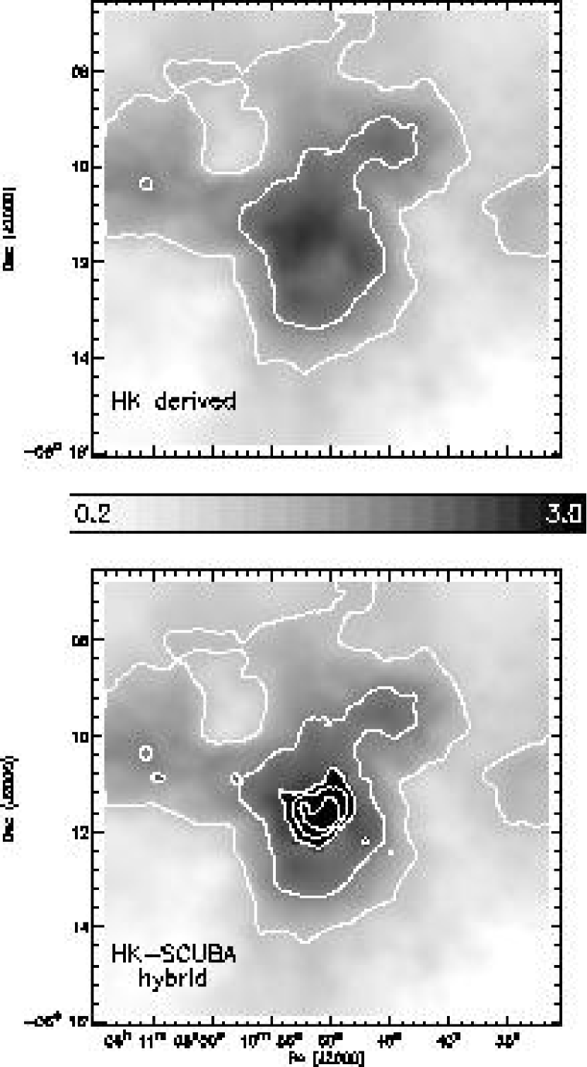
Figure 1.— Maps of $A_{K}$ as a function of position over the field of view of our near-IR observations of GGD 12-15. The top map is derived purely from the $H-K$ colors of all the stars detected in both bands. The bottom map is the same $HK$-derived map, updated with values derived from the SCUBA 850 $\mu$m maps in places where there is a clear underestimate in the $HK$-derived values. Note that these maps are log-scaled and inverted, with locations having $A_{K}<0.2$ in white and $A_{K}>3.0$ in black. The contour levels are $A_{K}=0.6,1.2,2.4,4.8,9.6$.

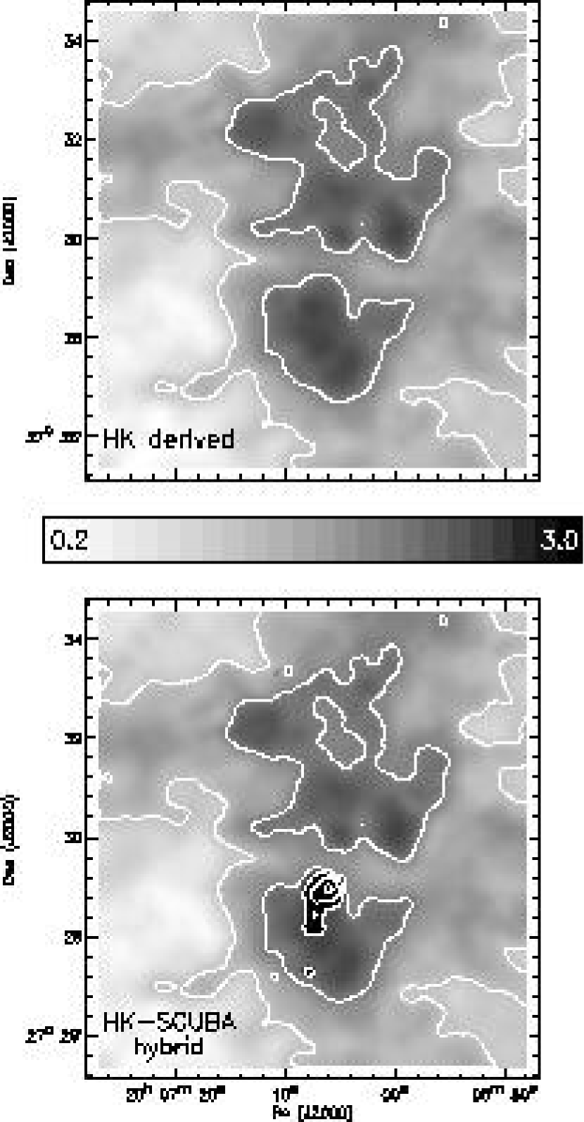
Figure 2.— Maps of $A_{K}$ as a function of position over the field of view of our near-IR observations of IRAS 20050+2720. For a detailed description, see Fig. 1.

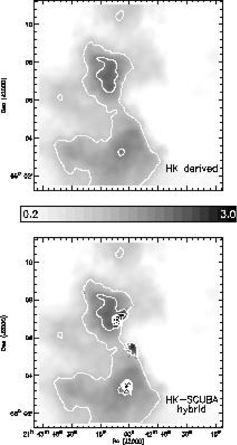
Figure 3.— Maps of $A_{K}$ as a function of position over the field of view of our near-IR observations of NGC 7129. For a detailed description, see Fig. 1.

Table 3Cluster core characteristics.

	GGD 12-15	IRAS 20050+2720	NGC 7129
Cluster-Dominated Region Radius (pc):	0.29	0.29	0.59
Cluster Core Radius (pc):	0.24	0.24	0.65
No. of Cluster Region Members:	$98\pm 10$	$91\pm 10$	$122\pm 16$
No. of Cluster Region Field Stars:	$15\pm 2$	$58\pm 4$	$114\pm 8$
Azimuthal Asymmetry Parameter:	1.588	1.421	1.207
Peak Surface Density (pc-2):	5910	6320	2750
Mean Surface Density (pc-2):	371	344	91.9
Peak Volume Density (pc-3):	$2.7\times 10^{5}$	$3.0\times 10^{5}$	$8.6\times 10^{4}$
Mean Volume Density (pc-3):	959	891	106

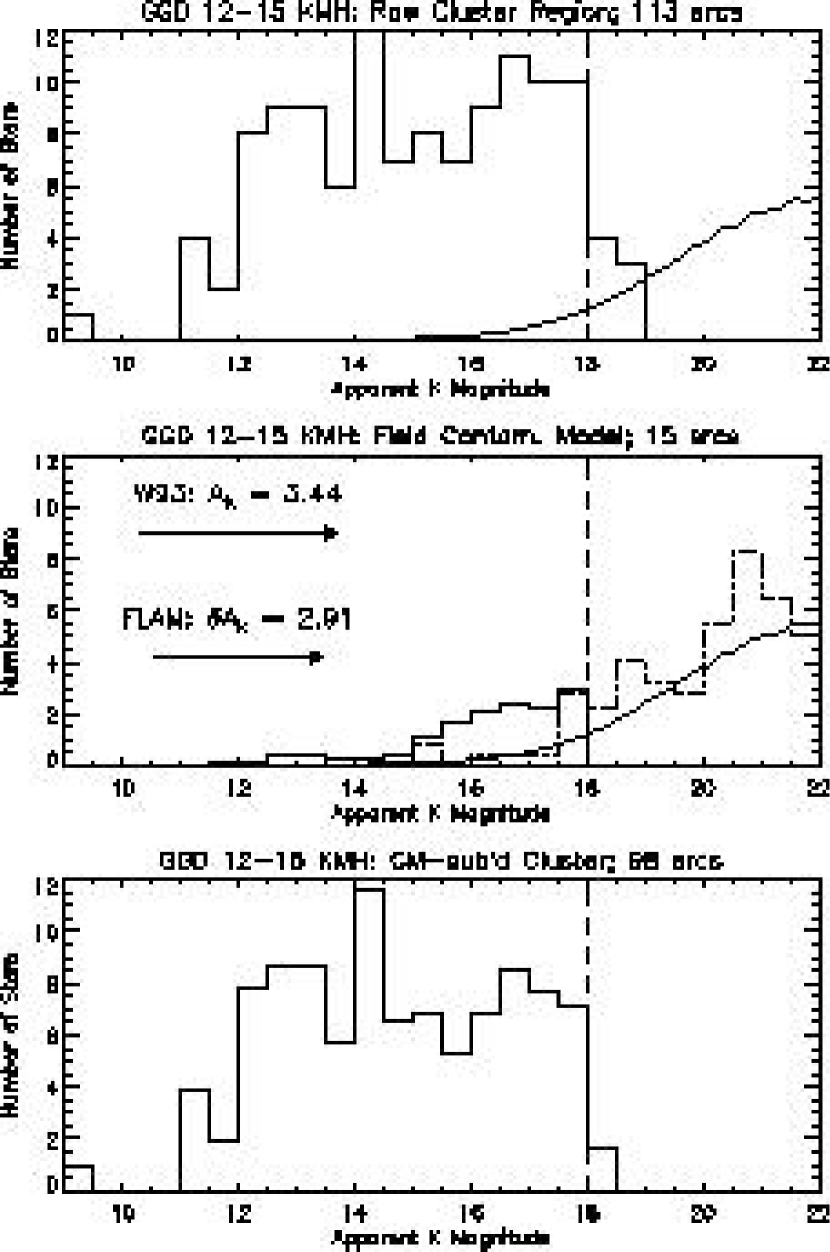
Figure 4.— $K$–band apparent magnitude histograms for GGD 12-15. The top plot consists of all stars detected within the cluster region boundary. The middle plot shows three field star KMH models. The dot-dashed line is the measured off-field KMH, shifted by $\delta A_{K}$ and scaled by the ratio of the areas of the cluster core and off-fields. The smooth, solid line overplotted on this and the first plot is the field star model of Wainscoat et al. (1993), shifted by the average $A_{K}$ of the cluster region, for comparison. The solid histogram is the mean KMH of the stars within the cluster core boundary from the $N_{CM}=1000$ Monte Carlo field star models generated in Section 3.2. The final plot is the difference of the raw cluster core histogram and a hybrid of the two field star KMHs derived from our observations. The mean Monte Carlo model KMH is used up to the limiting magnitude denoted by vertical dashed lines in all three plots. Beyond this limit, the scaled and shifted off-field KMH is used.

Figure 5.— Azimuthally averaged stellar radial density profiles for the GGD 12-15 region. The solid line histogram on the left shows the raw measured radial profile. The overplotted dot-dashed histogram is the mean radial profile from the $N_{CM}=1000$ Monte Carlo field star models. The solid line histogram on the right is the contamination–subtracted radial profile. Overplotted on both are smooth solid lines showing the exponential plus constant fits, vertical dashed lines marking the radii where the source counts are $3\sigma$ above the field star counts, and vertical dotted lines marking the cluster core radii, three times the e-folding lengths from the fits (see Section 3.3).

Figure 6.— TOP: Azimuthal distribution histograms of all stars within the cluster core boundary of GGD 12-15. The horizontal dashed line marks the mean number of stars per bin, corresponding to an ideally uniform stellar distribution for reference. The dot-dashed histogram plotted on the left is the mean azimuthal distribution of the $N_{CM}=1000$ Monte Carlo field star models. BOTTOM: Probability distribution histograms for the $AAP$ derived from $10^{6}$ model cluster fields (see Section 3.4). The left plot shows the raw $AAP$ distribution, and the right shows the $AAP$ after subtraction of the recentered mean azimuthal distribution of the field star models. Overplotted on both is a dashed line corresponding to a Gaussian of mean $|AAP_{sim}|$ and standard deviation $\sigma$ to demonstrate that the distributions are effectively approximated this way. Vertical dotted lines mark the location of the appropriate measured $AAP$.

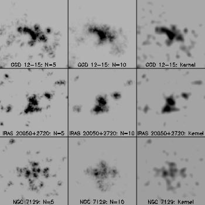
Figure 7.— Comparison of three different stellar surface density mapping methods for the three clusters presented: GGD 12-15, IRAS 20050+2720, and NGC 7129. In the left column are the $N=5$ stellar density maps used throughout this work (see Section 3.5). The maps in the central column are made with the same method, but the densities at each grid point are calculated using the distance to the nearest $N=10$ stars. Maps derived using Gaussian kernel smoothing (Gomez et al., 1993) with a smoothing width of $8^{\prime\prime}$ are in the right column. All maps are $5^{\prime}$ on a side.

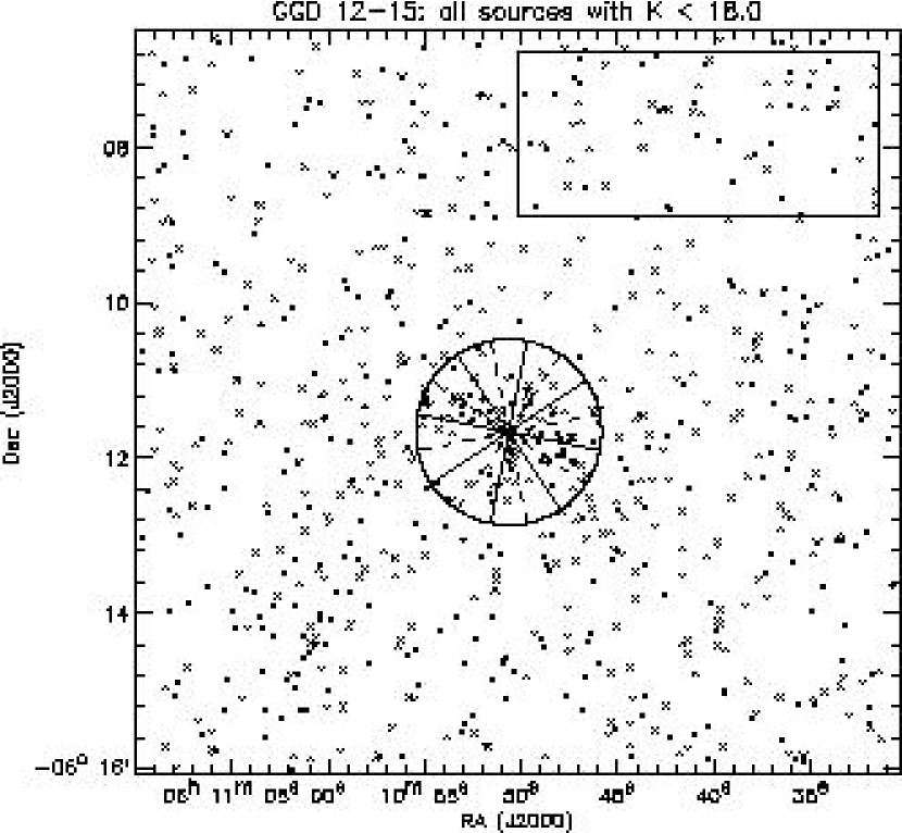
Figure 8.— Plot of all $K$–band detections brighter than $K=18$ in GGD 12-15. The box marks the off-field used for characterization of local field star contamination. The circle marks the cluster region boundary as determined in Fig. 5 (see Section 3.3). The overlapping $45^{\circ}$ position angle bins used to make the Nyquist sampled azimuthal distribution histograms in Fig. 6 are marked by the alternating black and gray wedge outlines.

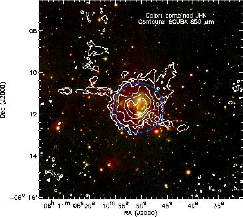
Figure 9.— $JHK$ log–scaled color image of the GGD 12-15 region from FLAMINGOS on MMT overlaid with 850 $\mu$m dust emission contours from SCUBA on JCMT. The contour levels start at 1.75 mJy pixel^-1 ($2^{\prime\prime}\times 2^{\prime\prime}$ pixels), with successive contour levels at double the previous level. The blue circle shows the cluster region boundary determined in Fig. 5.

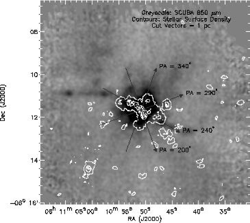
Figure 10.— 850 $\mu$m SCUBA map of GGD 12-15 in negative grayscale, scaled to show faint filamentary structure. Stellar surface density contours measured from all $K$–band point sources brighter than $K=18$ are overlaid. Contours begin at 435 pc^-2 ($5\sigma$ above median field star density), and increase at an interval of 750 pc^-2. The vectors denote the location and extent of the stellar surface density map cuts plotted in Fig. 11. Each vector is 1 pc in length at the assumed distance of 830 pc, approximately the distance a star moving $1kms^{-1}$ will travel in 1 Myr.

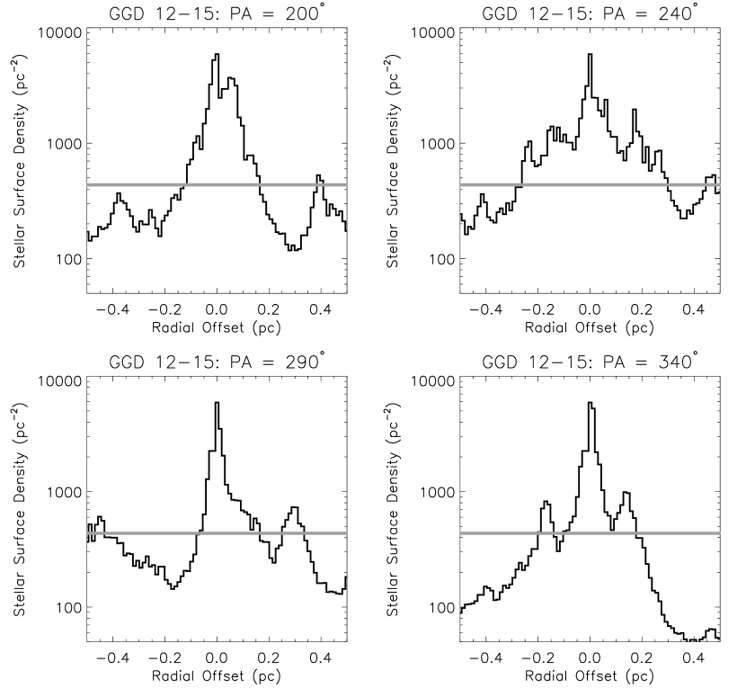
Figure 11.— The black lines in the above plots are stellar surface density map cuts for GGD 12-15. The vectors plotted in Fig. 10 mark the position, orientation, and direction of increasing offset from cluster center. Note the strong central peak, multiple sub-peaks, and lack of uniform circular symmetry. The gray line marks the $5\sigma$ above median field star density level for comparison, which corresponds to the first contour level in Fig. 10.

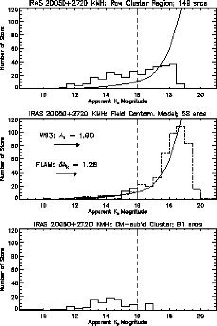
Figure 12.— $K_{s}$–band apparent magnitude histograms for IRAS 20050+2720. For a detailed description, see Fig. 4.

Figure 13.— Azimuthally averaged stellar radial density profiles for the IRAS 20050+2720 region. For a detailed description, see Fig. 5.

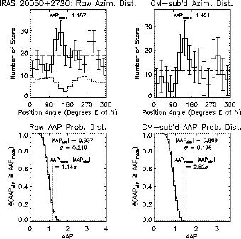
Figure 14.— Azimuthal distribution histograms and $AAP$ probability distribution histograms for IRAS 20050+2720. For a detailed description, see Fig. 6.

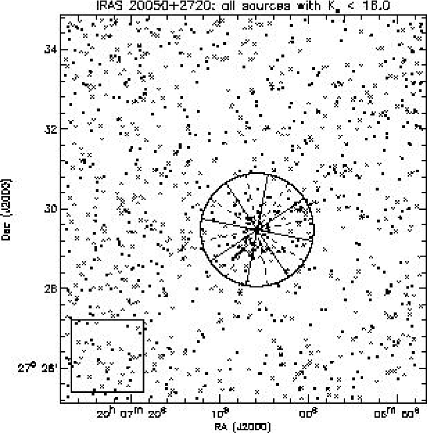
Figure 15.— Plot of all $K_{s}$–band detections brighter than $K_{s}=16$ in IRAS 20050+2720. The box marks the off-field used for characterization of local field star contamination. The circle marks the cluster region boundary as determined in Fig. 13 (see Section 3.3). The overlapping $45^{\circ}$ positional angle bins used to make the Nyquist sampled azimuthal distribution histograms in Fig. 14 are marked by the alternating black and gray wedge outlines.

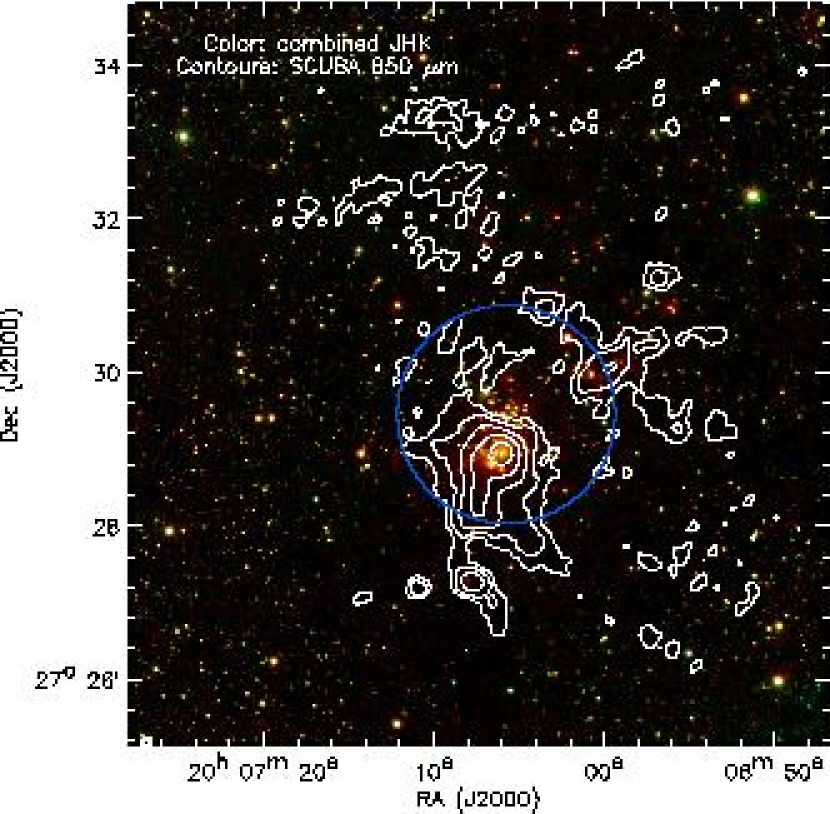
Figure 16.— $JHK_{s}$ log–scaled color image of the IRAS 20050+2720 region from FLAMINGOS on MMT overlaid with 850 $\mu$m dust emission contours from SCUBA on JCMT. The contour levels start at 1.75 mJy pixel^-1 ($2^{\prime\prime}\times 2^{\prime\prime}$ pixels), with successive contour levels at two times the previous level. The blue circle shows the cluster region boundary determined in Fig. 13.

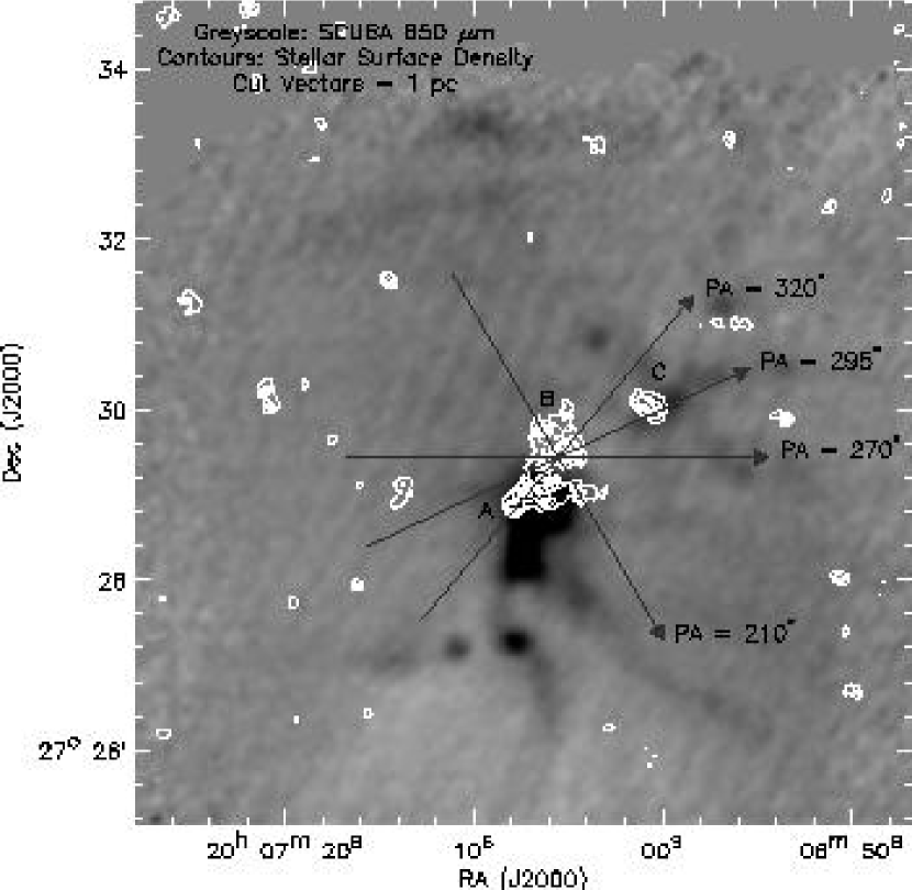
Figure 17.— 850 $\mu$m SCUBA map of IRAS 20050+2720 in negative grayscale, scaled to show faint filamentary structure. Stellar surface density contours measured from all $K_{s}$–band point sources brighter than $K_{s}=16$ are overlaid. Contours begin at 1450 pc^-2 ($5\sigma$ above median field star density), and increase at an interval of 750 pc^-2. The vectors denote the location and extent of the stellar density map cuts plotted in Fig. 18. Each vector is 1 pc in length at the assumed distance of 700 pc, approximately the distance a star moving $1kms^{-1}$ will travel in 1 Myr. The letters A, B, and C denote the contour groups that correspond to the three subclusters given those names by Chen et al. (1997).

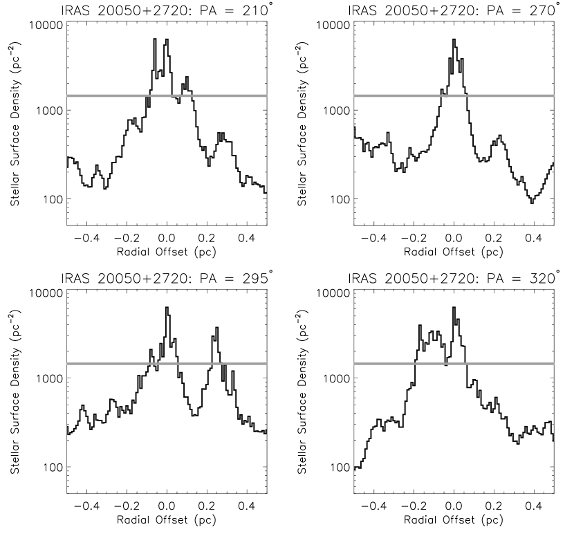
Figure 18.— The black lines in the above plots are stellar surface density map cuts for IRAS 20050+2720. The vectors plotted in Fig. 17 mark the position, orientation, and direction of increasing offset from cluster center. Note the multiple strong peaks and deviation from circular symmetry. The gray line marks the $5\sigma$ above median field star density level for comparison, which corresponds to the first contour level in Fig. 17.

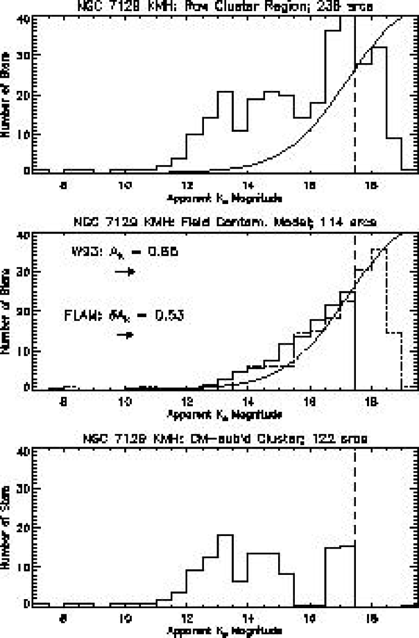
Figure 19.— $K_{s}$–band apparent magnitude histograms for NGC 7129. For a detailed description, see Fig. 4.

Figure 20.— Azimuthally averaged stellar radial density profiles for the NGC 7129 region. For a detailed description, see Fig. 5.

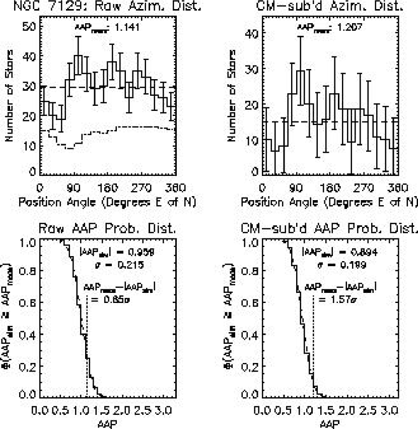
Figure 21.— Azimuthal distribution histograms and $AAP$ probability distribution histograms for NGC 7129. For a detailed description, see Fig. 6.

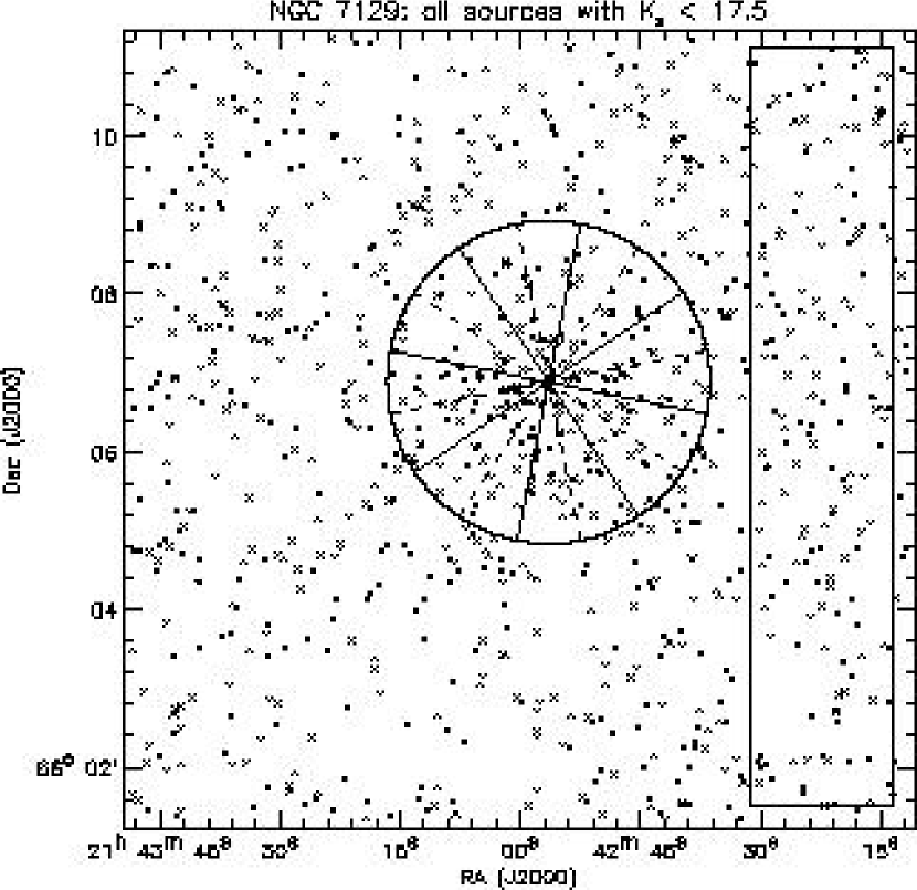
Figure 22.— Plot of all $K_{s}$–band detections brighter than $K_{s}=17.5$ in NGC 7129. The box marks the off-field used for characterization of local field star contamination. The circle marks the cluster region boundary as determined in Fig. 20 (see Section 3.3). The overlapping $45^{\circ}$ positional angle bins used to make the Nyquist sampled azimuthal distribution histograms in Fig. 21 are marked by the alternating black and gray wedge outlines.

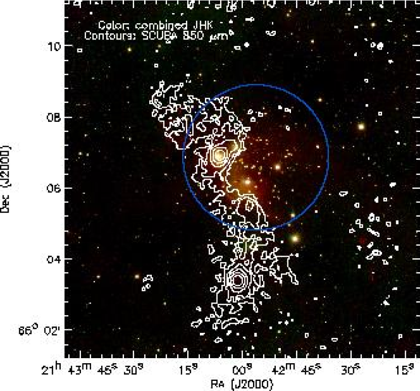
Figure 23.— $JHK_{s}$ log–scaled color image of the NGC 7129 region from FLAMINGOS on MMT overlaid with 850 $\mu$m dust emission contours from SCUBA on JCMT. The contour levels start at 1.75 mJy pixel^-1 ($2^{\prime\prime}\times 2^{\prime\prime}$ pixels), with successive contour levels at double the previous level. The blue circle shows the cluster region boundary determined in Fig. 20.

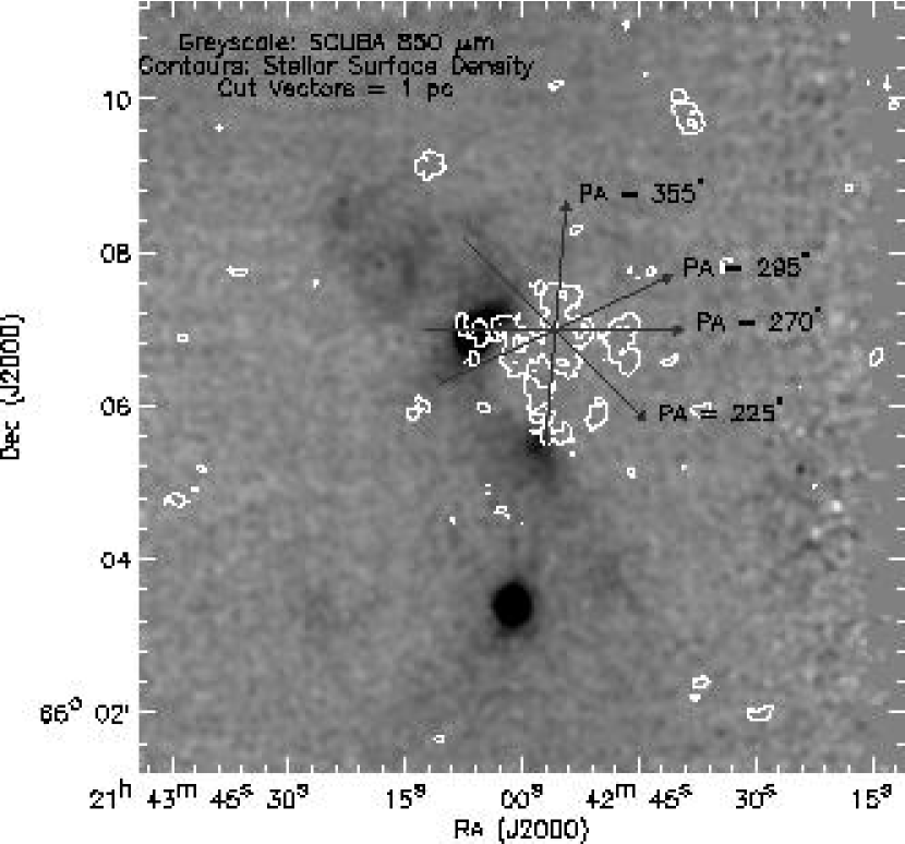
Figure 24.— 850 $\mu$m SCUBA map of NGC 7129 in negative grayscale, scaled to show faint filamentary structure. Stellar surface density contours measured from all $K_{s}$-band point sources brighter than $K_{s}=17.5$ are overlaid. Contours begin at 475 pc^-2 ($5\sigma$ above median field star density), and increase at an interval of 750 pc^-2. The vectors denote the location and extent of the stellar density map cuts plotted in Fig. 25. Each vector is 1 pc in length at the assumed distance of 1 kpc, approximately the distance a star moving $1kms^{-1}$ will travel in 1 Myr.

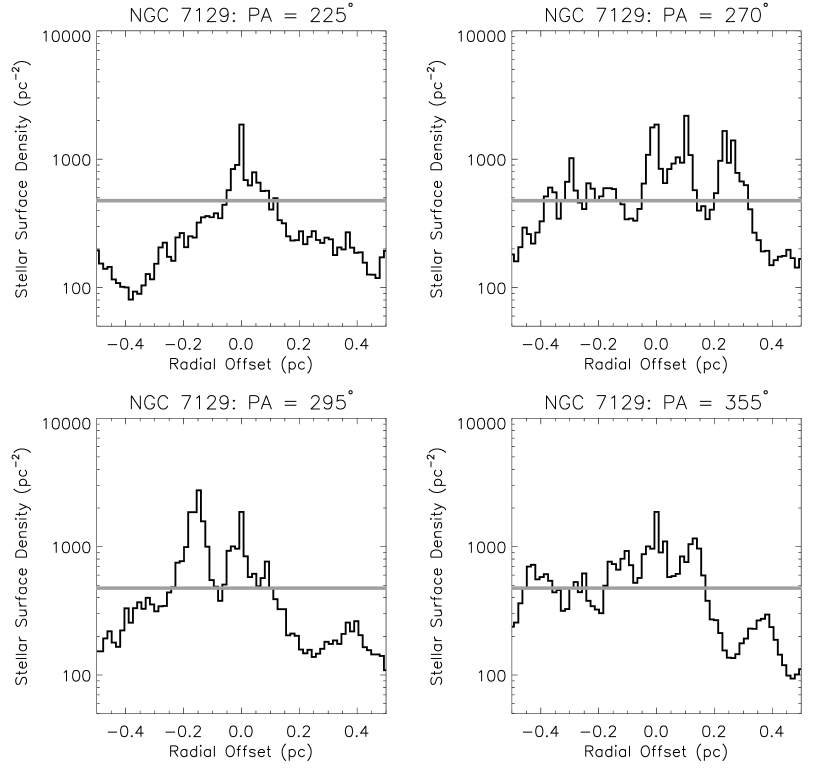
Figure 25.— The black lines in the above plots are stellar surface density map cuts for NGC 7129. The vectors plotted in Fig. 24 mark the position, orientation, and direction of increasing offset from cluster center. Note the lack of a cohesive peak and overall diffuse structure. The gray line marks the $5\sigma$ above median field star density level for comparison, which corresponds to the first contour level in Fig. 24.

Figure 26.— Estimates for collisional timescales for protostellar envelopes ($R=10^{3}$ AU, solid line) and T Tauri disks ($R=10^{2}$ AU, dashed line) as a function of stellar volume density.

Table 4Nearest Neighbor Volume Density Environments by Cluster

	GGD 12-15	IRAS 20050+2720	NGC 7129
No. of Stars at $>10^{4}$ pc-3:	74	100	35
Est. No. of Field Stars:	3	17	6
No. of Members at $>10^{4}$ pc-3:	71	83	29
Fraction of total in core:	72.4%	91.2%	23.8%

References

- Adams & Myers (2001) Adams, F. C., & Myers, P. C., 2001, ApJ, 553, 744
- Armitage, Clarke, & Palla (2003) Armitage, P. J., Clarke, C. J., & Palla, F., 2003, MNRAS, 342, 1139
- Bachiller, Fuente, & Tafalla (1995) Bachiller, R., Fuente, A., & Tafalla, M., 1995, ApJ, 445, L51
- Bate, Bonnell, & Bromm (2003) Bate, M. R., Bonnell, I. A., & Bromm, V., 2003, MNRAS, 339, 577
- Bechis et al. (1978) Bechis, K. P., Harvey, P. M., Campbell, M. F., & Hoffmann, W. F., 1978, ApJ, 226, 439
- Bertoldi & McKee (1992) Bertoldi, F. & McKee, C. F., 1992, ApJ, 395, 140
- Binney & Tremaine (1987) Binney, J., Tremaine, S., 1987, Galactic Dynamics, Princeton University Press, Princton, New Jersey
- Boffin et al. (1998) Boffin, H. M. J., Watkins, S. J., Bhattal, A. S., Francis, N., & Whitworth, A. P., 1998, MNRAS, 300, 1189
- Bonnell & Bate (2002) Bonnell, I. A., & Bate, M. R., 2002, MNRAS, 336, 659
- Bonnell, Bate, & Vine (2003) Bonnell, I. A., Bate, M. R., & Vine, S. G., 2003, MNRAS, 343, 413
- Boss (2002) Boss, A. P., 2002, ApJ, 576, 462
- Brown, Trujillo, & Rabinowitz (2004) Brown, M. E., Trujillo, C., & Rabinowitz, D., 2004, astro-ph/0404456
- Cabrit et al. (1997) Cabrit, S., Lagage, P.-O., McCaughrean, M., Olofsson, G., 1997, A&A, 321, 523
- Cardelli, Clayton, & Mathis (1989) Cardelli, J. A., Clayton, G. C., & Mathis, J. S., 1989, ApJ, 345, 245
- Carpenter et al. (1997) Carpenter, J. M., Meyer, M. R., Dougados, C., Strom, S. E., & Hillenbrand, L. A., 1997, AJ, 114, 198
- Carpenter (2000) Carpenter, J. M., 2000, ApJ, 120, 3139
- Chen et al. (1997) Chen, H., Tafalla, M., Greene, T. P., Myers, P. C., & Wilner, D. J., 1997, ApJ, 475, 163
- Chini et al. (2001) Chini, R., Ward-Thompson, D., Kirk, J. M., Nielbock, M., Reipurth, B., & Sievers, A., 2001, A&A, 369, 155
- Christopher et al. (1998) Christopher, M., Myers, P. C., Allen, L., Di Francesco, J., & Megeath, S. T., 1998, AAS, 193.6706
- Cohen et al. (1981) Cohen, J. G., Persson, S. E., Elias, J. H., & Frogel, J. A., 1981, ApJ, 249, 481
- D’Alessio et al. (2004) D’Alessio, P., et al., 2004, submitted to ApJ
- Edwards & Snell (1983) Edwards, S., & Snell, R. L., 1983, ApJ, 270, 605
- Eiroa, Palacios, & Casali (1998) Eiroa, C., Palacios, J., & Casali, M. M., 1998, A&A, 335, 243
- Eislöffel (2000) Eislöffel, J., 2000, A&A, 354, 236
- Elston (1998) Elston, R., 1998, Proc. SPIE, 3352, 328, Advanced Technology Optical/IR Telescopes VI, Larry M. Stepp, ed.
- Font, Mitchell, & Sandell (2001) Font, A. S., Mitchell, G. F., Sandell, G., 2001, ApJ, 555, 950
- Forrest et al. (2004) Forrest, W. J., et al., 2004, ApJS, 154, 443
- Fuente et al. (2001) Fuente, A., Neri, R., Martin-Pintado, J., Bachiller, R., Rodriguez-Franco, A., & Palla, F., 2001, A&A, 366, 873
- Gammie et al. (2003) Gammie, C. F., Lin, Y.-T., Stone, J. M., & Ostriker, J. P., 2003, ApJ, 592, 203
- Gladwin et al. (1999) Gladwin, P. P., Kitsionas, S., Boffin, H. M. J., & Whitworth, A. P., 1999, MNRAS, 302, 305
- Gomez et al. (1993) Gomez, M., Hartmann, L., Kenyon, S. J., & Hewett, R., 1993, AJ, 105, 1927
- Gómez, Rodríguez, & Garay (2000) Gómez, Y., Rodríguez, L. F., & Garay, G., 2000, ApJ, 531, 861
- Gómez, Rodríguez, & Garay (2002) Gómez, Y., Rodríguez, L. F., & Garay, G., 2002, ApJ, 571, 901
- Gutermuth et al. (2004) Gutermuth, R. A., Megeath, S. T., Muzerolle, J., Allen, L. E., Pipher, J. L., Myers, P. C., Fazio, G. G., 2004, ApJS, 154, 374
- Gyulbudaghian, Glushkov, & Denisyuk (1978) Gyulbudaghian, A. L., Glushkov, Y. I., & Denisyuk, E. K., 1978, ApJ, 224, L137
- Hartigan & Lada (1985) Hartigan, P., & Lada, C. J., 1985, ApJS, 59, 383
- Herbst & Racine (1976) Herbst, W., & Racine, R., 1976, AJ, 81, 840
- Hillenbrand (1995) Hillenbrand, L. A., 1995, Ph.D. Thesis, University of Massachusetts, Amherst
- Hodapp (1994) Hodapp, K. W. 1994, ApJS, 94, 615
- Jenness, Lightfoot, & Holland (1998) Jenness, T., Lightfoot, J. F., & Holland, W. S., 1998, Proc. SPIE, 3357, 548, Advanced Technology MMW, Radio, and Terahertz Telescopes, Thomas G. Phillips, ed.
- Kenyon & Hartmann (1995) Kenyon, S. J., & Hartmann, L. W., 1995, ApJS, 101, 117
- Klessen & Burkett (2000) Klessen, R. S., & Burkett, A., 2000, ApJS, 128, 287
- Klessen, Heitsch, & Mac Low (2000) Klessen, R. S., Heitsch, F., & Mac Low, M.-M., 2000, ApJ, 535, 887
- Kroupa, Petr, & McCaughrean (1999) Kroupa, P., Petr, M. G., & McCaughrean, M. J., 1999, New Astronomy, 4, 495
- Lada & Lada (2003) Lada, C. J., & Lada E. A., 2003, ARA&A, 41, 57
- Lada et al. (1994) Lada, C. J., Lada, E. A., Clemens, D. P., & Bally J., 1994, ApJ, 429, 694
- Lada (1992) Lada, E. A., 1992, ApJ, 393, L25
- Landsman (1993) Landsman, W. B, 1993, Astronomical Data Analysis Software and Systems II, A.S.P. Conference Series, Vol. 52, ed. R. J. Hanisch, R. J. V. Brissenden, and Jeannette Barnes, p. 246
- Lombardi & Alves (2001) Lombardi, M., & Alves, J., 2001, A&A, 377, 1023
- Li et al. (2004) Li, P. S., Norman, M. L., Mac Low, M.-M., & Heitsch, F., ApJ, 605, 800
- Little, Heaton, & Dent (1990) Little, L. T., Heaton, B. D., & Dent, W. R. F., 1990, A&A, 232, 173
- Luhman et al. (2003) Luhman, K. L., Stauffer, J. R., Muench, A. A., Rieke, G. H., Lada, E. A., Bouvier, J., & Lada, C. J., 2003, ApJ, 593, 1093
- McCaughrean & O’Dell (1996) McCaughrean, M. J., & O’Dell, C. R., 1996, AJ, 111, 1977
- Megeath (1994) Megeath, S. T., 1994, The Structure and Content of Molecular Clouds, Proceedings of a Conference Held at Schloss Ringberg, Tegernsee, Germany, 14-16 April 1993. Lecture Notes in Physics, Vol. 439, edited by T. L. Wilson and K. J. Johnston. Springer-Verlag, Berlin Heidelberg New York, p.215
- Megeath et al. (2002) Megeath, S. T., Biller, B., Dame, T. M., Leass, E., Whitaker, R. S., & Wilson, T. L., 2002, Hot Star Workshop III: The Earliest Stages of Massive Star Birth. ASP Conference Proceedings, Vol. 267. edited by Paul A. Crowther. ISBN: 1-58381-107-9. San Francisco, Astronomical Society of the Pacific, p.257
- Megeath et al. (2004) Megeath, S. T., Gutermuth, R. A., Allen, L. E., Pipher, J. L., Myers, P. C., & Fazio, G. G., 2004, ApJS, 154, 367
- Muench et al. (2002) Muench, A. A., Lada, E. A., Lada, C. J., & Alves, J., 2002, ApJ, 573, 366
- Miskolczi et al. (2001) Miskolczi, B., Tothill, N. F. H., Mitchell, G. F., Matthews, H. E., 2001, ApJ, 560, 841
- Motte & André (2001) Motte, F., & André, P., 2001, A&A, 365, 440
- Muzerolle et al. (2004) Muzerolle, J., et al., 2004, ApJS, 154, 379
- Palla & Stahler (2000) Palla, F., & Stahler, S. W., 2000, ApJ, 540, 255
- Persi & Tapia (2003) Persi, P., & Tapia, M., 2003, A&A, 406, 149
- Pfalzner et al. (2005) Pfalzner, S., Vogel, P., Scharwächter, J., & Olczak, C., 2005, astro-ph/0504288
- Pollack et al. (1994) Pollack, J. B., Hollenbach, D., Beckwith, S., Simonelli, D. P., Roush, T., & Fong, W., 1994, ApJ, 421, 615
- Porras et al. (2003) Porras, A., Christopher, M., Allen, L., Di Francesco, J., Megeath, S. T., & Myers, P. C., 2003, AJ, 126, 1916
- Racine (1968) Racine, R., 1968, AJ, 73, 233
- Ray et al. (1990) Ray, T. P., Poetzel, R., Solf, J., & Mundt, R., 1990, ApJ, 357, L45
- Ridge et al. (2003) Ridge, N. A.. Wilson, T. L., Megeath, S. T., Allen, L. E., Myers, P. C., 2003, AJ, 126, 286.
- Rodríguez et al. (1980) Rodríguez, L. F., Moran, J. M., Gottlieb, E. W., & Ho, P. T. P., ApJ, 235, 845
- Testi, Palla, & Natta (1999) Testi, L., Palla, F., & Natta, A., 1999, A&A, 342, 515
- Wainscoat et al. (1993) Wainscoat, R. J., Cohen, M., Volk, K., Walker, H. J., & Schwartz, D. E., 1993, ApJS, 83, 111
- Weintraub et al. (1996) Weintraub, D. A., Kastner, J. H., Gatley, I., & Merrill, K. M., 1996, ApJ, 468, L45
- Whitney et al. (2004) Whitney, B. A., et al., 2004, ApJS, 154, 315
- Wilking et al. (1989) Wilking, B. A., Blackwell, J. H., Mundy, L. G., & Howe, J. E., 1989, ApJ, 345, 257