Effect of congestion costs on shortest paths through complex networks

Abstract

We analyze analytically the effect of congestion costs within a physically relevant, yet exactly solvable network model featuring central hubs. These costs lead to a competition between centralized and decentralized transport pathways. In stark contrast to conventional no-cost networks, there now exists an optimal number of connections to the central hub in order to minimize the shortest path. Our results shed light on an open problem in biology, informatics and sociology, concerning the extent to which decentralized versus centralized design benefits real-world complex networks.

PACS numbers: 87.23.Ge, 05.70.Jk, 64.60.Fr, 89.75.Hc

The interplay between structure and function in complex networks, has become a major research topic in physics, biology, informatics, and sociology watts98 ; nets ; nets2 ; charges ; central ; search ; gradient . For example, the very same links, nodes and hubs that help create short-cuts in space for transport, may become congested due to increased traffic yielding an increase in transit time charges . Unfortunately there are very few analytic results available concerning network congestion and optimal pathways in real-world networks charges ; central ; search ; gradient .

In this paper, we provide exact analytic results for the effects of congestion costs in networks with a combined ring-and-star topology. Figure 1(a) shows an example of our model network with $N=1$ central hub. In addition to the fact that it is analytically tractable and posseses a topology which is distinct from Refs. charges ; central ; search ; gradient , our model network is of direct relevance to a wide range of biological, computational and socio-economic systems in which there is a potentially congested central node(s). Figure 1(b) shows the nutrient transport in a laboratory-grown fungus appl . The major transport pathways pass through a central hub (i.e. centralized transport) with some minor pathways around it (i.e. decentralized transport). It is an important yet open question in biology as to how organisms such as fungi make a trade-off between centralized and decentralized transport, communication and control. A related scenario with a similar topology, concerns the new congestion charge scheme in London which aims to dissuade drivers from passing through the central zone. Airlines must balance the costs and benefits of stopovers at major, yet potentially overcrowded, airport hubs. Similar trade-offs between centralized and decentralized routing, communication and control arise in data networks, manufacturing supply-chains, and government. Even for crime or terrorist networks, one can ask how the Mafia’s approach of passing all decisions through a central ‘Godfather’ compares to the apparently headless form of modern terrorist cells. More generally, our model network could be used to describe clusters or motifs within larger networks in which relatively isolated hubs are connected to lower-connectivity nodes (e.g. scale-free network).

Figure 1: (Color online) (a) Our model network showing transport pathways through the central hub (connections of length $1/2$ denoted by thick lines) and around the ring (connections of length $1$ denoted by thin lines). Graph shows average shortest path length between any two nodes in a $n=1000$ node ring, with a cost-per-connection to the hub of $k=1$. There is an optimal value for the number of connections ($\rho\equiv pn\approx 44$) such that the average shortest path length $\bar{\ell}$ is a minimum. We denote this minimal shortest path length as $\bar{\ell}\equiv\bar{\ell}|_{\rm min}$. (b) Photon scintillation image showing the nutrient distribution within a laboratory-grown fungus Phanerochaete velutina. Nutrient density increases going from blue to green to red.

Our model represents a generalization of Ref. DM to the case of non-zero congestion costs. Each of the $n$ nodes around the ring is connected to its nearest neighbors by a link of unit length. These links are directed in the ‘directed’ model, and undirected in the ‘undirected’ model. With a probability $p$ any node can be attached to the central hub by a link of length $\frac{1}{2}$. The links to the hub are always undirected. For both the directed and undirected models, explicit expressions can be derived for the probability $P(\ell,m)$ that the shortest path between any two nodes on the ring is $\ell$, given that they are separated around the ring by length $m$. Summing over all $m$ for a given $\ell$ and dividing by $(n-1)$ yields the probability $P(\ell)$ that the shortest path between two randomly selected nodes is of length $\ell$. The average value for the shortest path across the network is then $\bar{\ell}=\sum_{\ell=1}^{n-1}\ell P(\ell)$. For the undirected model, the expressions are more cumbersome because there are more paths with the same length. However, defining $nP(\ell)\equiv Q(z,\rho)$ where $\rho\equiv pn$ and $z\equiv\ell/n$, there is a simple relationship between the undirected and directed models in the limit $n\rightarrow\infty$ with $p\rightarrow 0$, i.e. $Q_{undir}(z,\rho)=2Q_{dir}(2z,\rho)$ DM . The models only differ in this limit by a factor of two: $z\rightarrow 2z$, with $z$ now running from $0$ to $1/2$. The results which follow were obtained by generalizing this procedure.

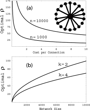
Figure 2: Minimal shortest path length $\bar{\ell}|_{\rm min}$ (i.e. minimum value of $\bar{\ell}$) as obtained from Eq. (Effect of congestion costs on shortest paths through complex networks). (a) Optimal number of connections $\rho\equiv pn$ as a function of the cost-per-connection $k$ to the hub. Results are shown for $n=1000$ and $n=10000$. (b) Optimal number of connections $\rho$ as a function of the network size. Results are shown for $k=2$ and $k=4$.

We add a cost $c$ every time a path passes through the central hub. This cost $c$ is expressed as an additional path-length, however it could also be expressed as a time delay or reduction in flow-rate for transport and supply-chain problems. We consider three cases: (1) constant cost $c$ where $c$ is independent of how many connections the hub already has, i.e. $c$ is independent of how ‘busy’ the hub is; (2) linear cost $c$ where $c$ grows linearly with the number of connections to the hub, and hence varies as $\rho\equiv np$; (3) nonlinear cost $c$ where $c$ grows with the number of pairs connected directly across the network, and hence varies as $\rho^{2}$.

For a general, non-zero cost $c$ that is independent of $\ell$ and $m$, we can write (for a network with directed links):

$$P(\ell,\ell\leq c) = \frac{1}{n-1}$$ (1)

$$P(\ell<m,\ell>c) = (\ell-c)p^{2}(1-p)^{\ell-c-1}$$ (2)

$$P(\ell=m,\ell>c) = 1-p^{2}\sum_{i-c=1}^{\ell-c-1}(i-c)(1-p)^{(i-c)-1}$$ (3)

Performing the summation gives:

$$P(\ell=m,\ell>c)=(1+(\ell-c-1)p)(1-p)^{\ell-c-1}$$ (4)

The shortest path distribution is hence:

$$P(\ell)=\left\{\begin{array}[]{ll}\frac{1}{n-1}&\ \ \textrm{$\forall$ $\ell\leq c$}\\ \frac{1}{n-1}\bigl{[}1+(\ell-c-1)p\\ \ \ \ \ \ \ +(n-1-\ell)(\ell-c)p^{2}\bigr{]}(1-p)^{\ell-c-1}&\ \ \textrm{$\forall$ $\ell>c$}\end{array}\right.$$

Using the same analysis for undirected links yields a simple relationship between the directed and undirected models. Introducing the variable $\gamma\equiv\frac{c}{n}$ with $z$ and $\rho$ as before, we may define $nP(\ell)\equiv Q(z,\gamma,\rho)$ and hence find in the limit $p\rightarrow 0$, $n\rightarrow\infty$ that $Q_{undir}(z,\gamma,\rho)=2Q_{dir}(2z,2\gamma,\rho)$. For a fixed cost, not dependent on network size or the connectivity, this analysis is straightforward. Paths of length $l\leq c$ are prevented from using the central hub, while for $l>c$ the distribution $P(l)$ is similar to that of Ref. DM .

For linear costs, dependent on network size and connectivity and for $N=1$ central hub, we can show that there exists a minimum value of the average shortest path $\bar{\ell}$ as a function of the connectivity to the central hub. Hence there is an optimal number of connections to the central hub, in order to create the minimum possible average shortest path. We denote this minimal path length as $\bar{\ell}\equiv\bar{\ell}|_{\rm min}$. Such a minimum is in stark contrast to the case of zero cost per connection, where the value of $\bar{\ell}$ would just decrease monotonically towards one with an increasing number of connections to the hub. We now calculate the average shortest path, $\bar{\ell}=\sum_{\ell=1}^{n-1}\ell P(\ell)$, which yields:

$$\bar{\ell}=\frac{(1-p)^{n-c}\bigl{[}3+(n-2-c)p\bigr{]}}{p^{2}(n-1)}\ \ \ \ \ \ \ \ \ \ \ \ \ \ \ \ \ \ \ \ \ \ \$$

$$+\frac{p\bigl{[}2-2c+2n-(c-1)(c-n)p\bigr{]}-3}{p^{2}(n-1)}+\frac{c(c-1)}{2(n-1)}\ .$$ (5)

Figure 1 shows the functional form of $\bar{z}\equiv\frac{\bar{\ell}}{n}$ with a cost of $1$ unit path-length per connection to the hub (i.e. $c=knp=k\rho$, with $k=1$). The optimal number of connections in order that $\bar{\ell}$ is a minimum is approximately $44$ and depends on $n$. The corresponding minimal shortest path $\bar{\ell}|_{\rm min}$ is approximately 85. An analytic expression for $\bar{\ell}|_{\rm min}$ can be obtained by setting the differential of Eq. (Effect of congestion costs on shortest paths through complex networks) equal to zero. If $n$ is very large, one can introduce a higher cost without compromising the minimal shortest path $\bar{\ell}|_{\rm min}$ since in general the nodes are already much further from one another. We can also investigate how many connections we should make for a given cost and network size, in order to achieve the minimum possible shortest path $\bar{\ell}|_{\rm min}$. This is obtained by setting the differential of Eq. (Effect of congestion costs on shortest paths through complex networks) equal to zero and solving for $p$. Figure 2(a) shows analytic results for the optimal number of connections which yield the minimal shortest path $\bar{\ell}|_{\rm min}$, as a function of the cost per connection for a fixed network size. Figure 2(b) shows analytic results for the optimal number of connections which yield the minimal shortest path $\bar{\ell}|_{\rm min}$, as a function of the network size for a fixed cost per connection to the hub.

To gain insight into the underlying physics, we now make some approximations to the exact analytic expressions. For large $n$, or more importantly large $n-c$, the term $(1-p)^{n-c}\rightarrow e^{-\rho}$ in Eq. (Effect of congestion costs on shortest paths through complex networks). Provided that the cost per connection to the hub is not too high, the region containing the minimal shortest path $\bar{\ell}|_{\rm min}$ will be at a reasonably high $\rho$ (recall Fig. 1(a)). Hence we can neglect the exponential term and differentiate to find the minimum value of $\bar{\ell}$ with $c=knp=k\rho$. It is reasonable to assume that at fixed $k$, optimal $\rho$ will increase with $n$ like $n^{x}$ where $0<x\leq 1$. In particular, one obtains diffusive behavior whereby $x\sim 1/2$. Specifically, $\rho\approx\sqrt{\frac{2n}{k}}$. For a large network (i.e. large $n$), we have therefore obtained a simple relationship between the number of connections one should introduce in order to create the minimal average shortest path between any two nodes in the network, and the cost per connection to the hub. It can be shown by comparing to Figure 2, that this analytic scaling relation is accurate even down to $n\sim 10$, but is particularly good for $n$ larger than $10^{3}$.

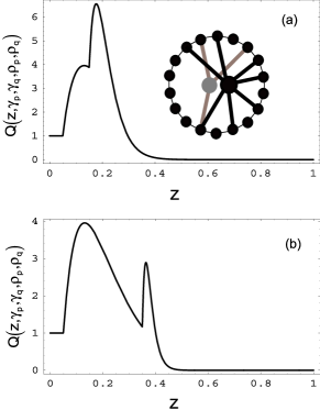
Figure 3: Examples of the scaled probability distribution for a network with $N=2$ hubs, where the two hubs have associated costs for travelling through them. In (a), $\rho_{p}=20$ and $\rho_{q}=10$ while the costs are $c_{p}=0.15$ and $c_{q}=0.05$. In (b), $\rho_{p}=50$ and $\rho_{q}=10$ while the costs are $c_{p}=0.35$ and $c_{q}=0.05$.

Now we briefly turn to consider a specific yet physically reasonable example of non-linear costs, in which the costs are taken to depend on the number of pairs which are connected via the hub. In particular, we use $c=k(np)^{2}$. We obtain the analytic relationship $\rho\approx\sqrt[3]{\frac{n}{k}}$ which is the non-linear equivalent of the above result. Obviously, more accurate expressions can be obtained since we know the complete form of the analytic solution – however these are too cumbersome algebraically to be presented here.

For linear costs, the lowest value of $\bar{\ell}$ one can achieve is $\bar{\ell}|_{\rm min}\approx\sqrt{8kn}$. Setting $n=10^{3}$ and $k=1$ gives $\bar{\ell}|_{\rm min}=89.4$, which agrees well with the exact analytic result shown in Fig. 1. For non-linear costs, the minimal shortest path $\bar{\ell}|_{\rm min}\approx\sqrt[3]{27kn^{2}}$. These last results show that the minimal shortest path $\bar{\ell}|_{\rm min}$ across the network grows like $n^{\frac{1}{2}}$ when we impose linear costs while it grows like $n^{\frac{2}{3}}$ when we put a cost on the number of direct connections between nodes made via the hub (i.e. non-linear costs). Corresponding results for the undirected model can be easily obtained from the equations for the directed model. For example for linear costs $c=knp$ and undirected links, we obtain $\bar{\ell}|_{\rm min}\approx\sqrt{4kn}$ and $\rho\approx\sqrt{\frac{n}{k}}$ for the minimal shortest path and the optimal connectivity.

The present analysis can be extended to multiple hubs, $N\geq 2$. For simplicity, we focus here on the specific example of constant costs and $N=2$ (i.e. hub P, with nodes connected to it with probability $p$ and hub Q, with nodes connected to it with probability $q$) where the cost associated with each hub has value $c_{p}$ and $c_{q}$, with $c_{p}\geq c_{q}$. The cost for using both hubs is assumed to be infinite. It is not hard to imagine real-world systems that employ multiple central hubs but which would not favour pathways through more than one at a time (e.g. an airline passenger would avoid buying a ticket with two stop-overs). Of course this assumption may not always be realistic (see, for example, Ref. railway ).

We first consider what happens when $\ell>c_{p}\geq c_{q}$. In this case, both hubs may be used and we may therefore write:

$$P(\ell<m) = P_{P}(\ell<m,\ell>c_{p})\bigl{[}1-\sum_{i-c_{q}=1}^{\ell-c_{q}-1}P_{Q}(i<m,i>c_{q})\bigr{]}$$ (6)

$$+ P_{Q}(\ell<m,\ell>c_{q})\bigl{[}1-\sum_{i-c_{p}=1}^{\ell-c_{p}-1}P_{P}(i<m,i>c_{p})\bigr{]}$$

$$- P_{P}(\ell<m,\ell>c_{p})P_{Q}(\ell<m,\ell>c_{q})$$

where $P_{P}(\ell<m,\ell>c_{p})$ and $P_{Q}(\ell<m,\ell>c_{q})$ are understood to be $P(\ell<m,\ell>c)$ from the single-hub-with-costs case for probabilities $p$ and $q$ respectively. Substituting Eq. (2) into the first term of Eq. (6) and performing the summation yields:

$$P_{P}(\ell<m,\ell>c_{p})\bigl{[}1-\sum_{i-c_{q}=1}^{\ell-c_{q}-1}P_{Q}(i<m,i>c_{q})\bigr{]}\ \ \ \ \ \ \$$

$$\ \ \ \ \ \ \ =(g_{0pq}+g_{1pq}\ell+g_{2pq}\ell^{2})(a_{p}a_{q})^{\ell-1}$$ (7)

where

$$a_{p} = 1-p$$

$$a_{q} = 1-q$$

$$g_{0pq} = (1-p)^{-c_{p}}(1-q)^{-c_{q}}p^{2}c_{p}((c_{q}+1)q-1)$$

$$g_{1pq} = (1-p)^{-c_{p}}(1-q)^{-c_{q}}p^{2}(1-(c_{p}+c_{q}+1)q)$$

$$g_{2pq} = (1-p)^{-c_{p}}(1-q)^{-c_{q}}p^{2}q\ \ .$$

An equivalent substitution and summation performed on the second term in Eq. (6) yields the same answer but with labels $p$ and $q$ interchanged. The third term, after substitution and summation, yields:

$$P_{P}(\ell<m,\ell>c_{p})P_{Q}(\ell<m,\ell>c_{q})\ \ \ \ \ \ \$$

$$\ \ \ \ \ \ \ =(h_{0}+h_{1}\ell+h_{2}\ell^{2})(a_{p}a_{q})^{\ell-1}$$ (8)

where

$$h_{0} = (1-p)^{-c_{p}}(1-q)^{-c_{q}}p^{2}q^{2}c_{p}c_{q}$$

$$h_{1} = -(1-p)^{-c_{p}}(1-q)^{-c_{q}}p^{2}q^{2}(c_{p}+c_{q})$$

$$h_{2} = (1-p)^{-c_{p}}(1-q)^{-c_{q}}p^{2}q^{2}\ \ .$$

Substitution of these individual terms into Eq. (6) yields:

$$P(\ell<m)=(g^{\prime}_{0}+g^{\prime}_{1}\ell+g^{\prime}_{2}\ell^{2})(a_{p}a_{q})^{\ell-1}$$ (9)

where $g^{\prime}_{i}=g_{ipq}+g_{iqp}-h_{i}$. To calculate the full probability distribution for the case $\ell>c_{p}\geq c_{q}$ we now only require $P(\ell=m)$:

$$P(\ell=m)=1-\sum_{i=c_{q}+1}^{c_{p}}P_{Q}(i<m)-\sum_{i=c_{p}+1}^{\ell-1}P(i<m)$$ (10)

where $P_{Q}(i<m)$ is the single-hub-plus-costs distribution for a hub with probability $q$ and $P(i<m)$ is given by Eq. (9). We define the following functions:

$$f_{x}(a,n) = \sum_{i=1}^{n-1}i^{x}a^{i-1}$$

$$\tilde{f}_{x}(a,n_{1},n_{2}) = f_{x}(a,n_{1})-f_{x}(a,n_{2})\ \ .$$

We then substitute $P_{Q}(i<m)$ and $P(i<m)$ into Eq. (10) yielding:

$$P(\ell=m,\ell>c_{p})=1-\frac{q^{2}}{(1-q)^{c_{q}}}\bigl{[}\tilde{f}_{1}(a_{q},c_{p}+1,c_{q}+1)$$

$$-c_{q}\tilde{f}_{0}(a_{q},c_{p}+1,c_{q}+1)\bigr{]}-\bigl{[}g^{\prime}_{0}\tilde{f}_{0}(a_{p}a_{q},\ell,c_{p}+1)$$

$$+g^{\prime}_{1}\tilde{f}_{1}(a_{q}a_{p},\ell,c_{p}+1)+g^{\prime}_{2}\tilde{f}_{2}(a_{p}a_{q},\ell,c_{p}+1)\bigr{]}\ \ .$$ (11)

We now obtain the final distribution by performing the sum over $m$:

$$P(\ell,\ell\leq c_{q})=\frac{1}{n-1}$$ (12)

$$P(\ell,c_{q}<\ell\leq c_{p})=\frac{1}{n-1}\bigl{[}1+(\ell-c_{q}-1)q$$

$$+(n-1-\ell)(\ell-c_{q})q^{2}\bigr{]}(1-q)^{\ell-c_{q}-1}$$ (13)

$$P(\ell,c_{p}<\ell)=\frac{1}{n-1}\biggl{[}1-\frac{q^{2}}{(1-q)^{c_{q}}}\bigl{[}\tilde{f}_{1}(a_{q},c_{p}+1,c_{q}+1)$$

$$-c_{q}\tilde{f}_{0}(a_{q},c_{p}+1,c_{q}+1)\bigr{]}-\bigl{[}g^{\prime}_{0}\tilde{f}_{0}(a_{p}a_{q},\ell,c_{p}+1)$$

$$+g^{\prime}_{1}\tilde{f}_{1}(a_{q}a_{p},\ell,c_{p}+1)+g^{\prime}_{2}\tilde{f}_{2}(a_{p}a_{q},\ell,c_{p}+1)\bigr{]}$$

$$+\bigl{[}(n-1-\ell)(g^{\prime}_{0}+g^{\prime}_{1}\ell+g^{\prime}_{2}\ell^{2})(a_{p}a_{q})^{\ell-1}\bigr{]}\biggr{]}\ \ \ \ .$$ (14)

The resulting distribution, which has an interesting multi-modal form, is plotted in Fig. 3 for the directed case: $Q$ now depends on five variables due to the additional probability $q$ and cost $c_{q}$, such that $\rho_{p}\equiv pn$, $\rho_{q}\equiv qn$, $\gamma_{p}\equiv\frac{c_{p}}{n}$, $\gamma_{q}\equiv\frac{c_{q}}{n}$ with $z$ as before. Interestingly if the value of $\rho_{q}$ increases above $\rho_{p}$ the distribution tends to the single hub case extremely quickly - i.e. the P-hub is then barely used. If the P-hub has a high degree and a high cost, then the distribution behaves as though the P-hub is not there until $\ell>\gamma_{p}$, where it quickly falls to zero. The undirected case is similar to the directed case since once again the same scaling relationship exists between them.

In summary, we have presented analytic results for a simple yet realistic model of a congested network. Elsewhere we will discuss embedding our $N$-hub cluster within larger and more complex networks, and will present a quantitative comparison to the transport routings observed within laboratory-grown fungi in an attempt to understand ‘costs’ within biological networks.

N.F.J. is grateful to P.M. Hui and F.J. Rodriguez for discussions, and thanks M. Tlalka, S.C. Watkinson, P.R. Darrah and M.D. Fricker for permission to use the image in Fig. 1(b).

References

• (1) D.J. Watts and S.H. Strogatz, Nature 393, 440 (1998).
• (2) D. S. Callaway, M. E. J. Newman, S. H. Strogatz, and D. J. Watts, Phys. Rev. Lett. 85, 5468 (2000).
• (3) R. Albert and A.L. Barabasi, Phys. Rev. Lett. 85, 5234 (2000).
• (4) L.A. Brunstein, S.V. Buldyrev, R. Cohen, S. Havlin and H.E. Stanley, Phys. Rev. Lett. 91, 168701 (2003).
• (5) R. Guimera, A. Diaz-Guilera et al., Phys. Rev. Lett. 89, 248701 (2002).
• (6) V. Colizza, J. R. Banavar et al., Phys. Rev. Lett. 92, 198701 (2004).
• (7) Z. Toroczkai, K. E. Bassler, Nature 428, 716 (2004).
• (8) M. Tlalka, D. Hensman, P.R. Darrah, S.C. Watkinson and M.D. Fricker, New Phytologist 158, 325 (2003).
• (9) S.N. Dorogovtsev and J.F.F. Mendes, Europhys. Lett. 50, 1 (2000).
• (10) P. Sen, S. Dasgupta, A. Chatterjee, P. A. Sreeram, G. Mukherjee and S. S. Manna, Phys. Rev. E 67, 036106 (2003).