Winning quick and dirty: the greedy random walk

Abstract

As a strategy to complete games quickly, we investigate one-dimensional random walks where the step length increases deterministically upon each return to the origin. When the step length after the $k^{\rm th}$ return equals $k$, the displacement of the walk $x$ grows linearly in time. Asymptotically, the probability distribution of displacements is a purely exponentially decaying function of $|x|/t$. The probability $E(t,L)$ for the walk to escape a bounded domain of size $L$ at time $t$ decays algebraically in the long time limit, $E(t,L)\sim L/t^{2}$. Consequently, the mean escape time $\langle t\rangle\sim L\ln L$, while $\langle t^{n}\rangle\sim L^{2n-1}$ for $n>1$. Corresponding results are derived when the step length after the $k^{\rm th}$ return scales as $k^{\alpha}$ for $\alpha>0$.

I Introduction

A popular card game for young children is “war”. The rules of this game are extremely simple: with two players, start by dividing the cards evenly between the players. At each play, the players expose the top card in their piles. The person with the higher card collects the two exposed cards and incorporates them into his or her pile. When there is a tie, a “war” ensues. Each player contributes three additional cards from his or her pile to the pot and then the fourth card is exposed. The winner takes the pot. In case of another tie, the war is repeated until there is a winner. The game ends when one player no longer has any cards.

Similar to many other games including for example, coin toss, roulette, and dreidel, the game of war resembles a random walk HG ; LPP ; DD , as the number of cards possessed by each player changes by $\pm 1$ (or by $\pm 5$, $\pm 9$, etc., when occasional wars occur) after each play. Since there are $N=52$ cards in a deck, a natural anticipation is that the length of the game scales as $N^{2}$ ruin ; RV . Based on soporific experiences in playing war with our children, it is desirable to modify the rules so that the game ends more quickly. We have found that the following modification – which we term “superwar” – works quite well: in each war, increase the number of cards that a player contributes to the pot by one compared to the previous war. This modification of war ends much more quickly than the original game and is also more exciting for young children.

The game of superwar inspires the present work in which we investigate the properties of a one-dimensional random walk in which the step length increases in a deterministic manner each time the walk returns to the origin. We term this process the Greedy Random Walk. More generally, we consider the situation where the step length $\ell_{k}$ after the $k^{\rm th}$ return to the origin is

$$\ell_{k}=k^{\alpha},$$ (1)

with positive $\alpha$; the initial step length equals one. The increasing step length corresponds to increasing the payoff when the cumulative score of a game is tied. This mechanism provides a strategy to complete games quickly, although it differs than superwar where the payoff is raised when there is a tie in a single play.

In the next section, we give heuristic arguments for the typical displacement and for extremal properties of the probability distribution. Then we study the probability distribution of the greedy walk in an infinite system. We present simulation results as well as an asymptotic solution for this distribution. Our solution relies heavily on classic first-passage properties of random walks F68 ; W ; fpp ; RG . The probability distribution of the greedy random walk has several intriguing non-scaling features, including sharp valleys at the prime numbers and an anomalous contribution due to walks that never return to the origin.

In Sec. III, we determine how long it take for a greedy walk to escape the finite interval $[-L,L]$. Generically, the escape time grows more slowly than the diffusive time scale $L^{2}/D$. As a consequence, the game ends much more quickly. However, the escape probability has a power-law tail so that the higher moments are controlled by the diffusive time scale. Thus the escape time of the greedy walk are characterized by large fluctuations.

II Displacement statistics

II.1 Typical and Extremal Displacements

We first determine the typical displacement of the greedy random walk. A crucial fact is that the statistics of returns to the origin are not affected by the growth of the step length. Thus, a typical walk of $t$ steps will visit the origin of the order of $k\sim t^{1/2}$ times F68 ; W ; fpp ; RG . Thus, the step length $\ell=k^{\alpha}$ grows as $t^{\alpha/2}$. For an ordinary random walk with step length $\ell$, the typical displacement is $x\sim t^{1/2}\ell$. Combining these two scaling laws, the typical displacement of the greedy walk grows with time as

$$x\sim t^{\nu},$$ (2)

with $\nu={(1+\alpha)/2}$. Thus the greedy walk is more extended than a conventional random walk.

We expect that this typical displacement characterizes the probability distribution that the greedy walk is at position $x$ at time $t$, $G(x,t)$. In the long time limit, this distribution should thus conform to the conventional scaling form

$$G(x,t)\simeq t^{-\nu}\Phi\left(x\,t^{-\nu}\right),$$ (3)

where $\Phi(z)$ is the scaling function.

We can determine the asymptotic decay of $\Phi(z)$ by using a Lifshitz tail argument MEF ; L . As a preliminary, we need to identify the walks with the maximal possible displacement. For conventional random walks, the extremal walk is ballistic – stepping in one direction only. For the greedy random walk, in contrast, extremal walks involve a compromise between returning to the origin often, so as to acquire a large single-step length, and moving in one direction, so as to be as far from the origin as possible. We are thus led to consider a hybrid zig-zag/ballistic walk that makes immediate reversals for the first $\tau$ steps and then moves in one direction for the remaining $t-\tau$ steps.

Figure 1: Extremal greedy walk of 16 steps when the step length grows linearly at each return to the origin. There are 4 immediate reversals in the first 8 steps and then the remaining steps are all in one direction.

When only immediate reversals in direction occur, the step length after $\tau$ steps ($\tau/2$ returns) is $\ell_{\tau/2}=(\tau/2)^{\alpha}$. Then if the remaining steps are all in one direction, the displacement of the walk at time $t$ is

$$x=(t-\tau)\,\left(\frac{\tau}{2}\right)^{\alpha}.$$ (4)

Maximizing this expression with respect to $\tau$, the optimum value of $\tau$ is $\tau=\frac{\alpha}{1+\alpha}\,t$ and the maximal displacement is

$$x_{\rm max}\propto t^{1+\alpha}.$$ (5)

Notice that the exponent characterizing the maximal displacement is twice that of the typical displacement, $x_{\rm max}\sim t^{2\nu}$.

We now exploit the result for $x_{\rm max}$ to estimate the tail of the probability distribution. We first make the standard assumption that the tail of the probability distribution decays as a stretched exponential, $\Phi(z)\sim\exp\left(-|z|^{\delta}\right)$, for $z\gg 1$ MEF , where all factors of order one have been ignored. With this ansatz, the probability for the maximal-displacement greedy walk asymptotically scales as

$$G(x=t^{2\nu},t)\sim\exp\left(-t^{\nu\delta}\right).$$ (6)

On the other hand, the probability for this maximal-displacement walk decays exponentially with time, since a finite fraction of the steps in the walk must be uniquely specified. Equating this exponential decay to the form given in Eq. (6), we immediately conclude that $\delta=1/\nu$. As a result, we deduce that the scaling function in $G(x,t)$ decays according to

$$\Phi(z)\sim\exp\left(-|z|^{2/(1+\alpha)}\right),$$ (7)

for $z\gg 1$. Notice that the conventional Fisher scaling relation $\delta=(1-\nu)^{-1}$ is violated for greedy walks MEF .

II.2 The Probability Distribution

We can obtain the full probability distribution of greedy walks by utilizing basic first-passage properties of ordinary random-walks. These first-passage techniques provide an insightful and pleasant way to understand greedy walks. There are two generic ways that the greedy walk can be at position $x$ at time $t$ when starting at the origin at $t=0$. The first is to reach $x$ without ever returning to the origin. The second possibility, as depicted in Fig. 2, is that the walk returns to the origin $k$ times, with the $k^{\rm th}$ return occurring at time $\tau$, and then the walk reaches $x$ in the remaining $t-\tau$ steps without touching the origin again. The number of returns to the origin is variable, but the maximum number cannot exceed $t/2$.

Figure 2: Space-time trajectory of an example greedy random walk, with 4 returns to the origin after $\tau$ steps. Upon each return, the step length increases, as indicated schematically. After the last return, the final position is reached in the remaining $t-\tau$ steps.

According to this decomposition of a greedy walk into a segment that consists of $k$ returns to the origin and a non-return segment, we can write the probability distribution of greedy walks in the following form:

$$G(x,t)=Q(x,t)+\sum_{k=1}^{k_{\rm max}}\int_{0}^{t}\!F^{(k)}(0,\tau)\,\frac{1}{k^{\alpha}}Q\!\left(\frac{x}{k^{\alpha}},t\!-\!\tau\right)d\tau.$$ (8)

Here $k_{\rm max}$ is the maximum possible number of returns to the origin in time $t$ when the final displacement is $x$. The first term on the right is the probability that a walk, which never returns to the origin, is at $x$ at time $t$. In the second term, $F^{(k)}(0,\tau)$ is the $k^{\rm th}$-passage probability to the origin, namely, the probability that the walk returns to the origin $k$ times, with the $k^{\rm th}$ return occurring at time $\tau$. The term $\frac{1}{k^{\alpha}}Q\left(\frac{x}{k^{\alpha}},t-\tau\right)$ then accounts for the probability for the walk to reach $x$ in the remaining $t-\tau$ steps without touching the origin again. Because the step length is $k^{\alpha}$ in this last leg of the walk, $x/k^{\alpha}$ steps are required to reach $x$. We also need to include the prefactor $1/k^{\alpha}$ to ensure proper normalization.

Since Eq. (8) is in the form of a convolution, it is much more convenient to work with Laplace transforms. Then the basic equation for the probability distribution simplifies to

$$G(x,s)=Q(x,s)+\sum_{k=1}^{k_{\rm max}}F^{(k)}(0,s)\,\,\frac{1}{k^{\alpha}}Q\left(\frac{x}{k^{\alpha}},s\right),$$ (9)

where the argument $s$ is generally used to signify Laplace transformed quantities. Each of the terms on the right-hand side of this equation are well known first-passage properties F68 ; W ; fpp ; RG , from which we can then obtain the probability distribution of greedy walks.

We now determine the individual terms that appear in Eq. (9). The non-return probability $Q(x,t)$ is the probability that a random walk, that starts at $x_{0}=1$, is at position $x$ at time $t$, and that the origin is never visited. In the $t\to\infty$ limit, this quantity satisfies the diffusion equation $Q_{t}=DQ_{xx}$ subject to the absorbing boundary condition $Q(x=0,t)=0$. This boundary condition ensures that only walks that do not hit the origin are counted. It is simple to construct $Q(x,t)$ by the image method. We merely place a random walk of opposite “charge” at $-x_{0}$; this construction ensures that the boundary condition at $x=0$ is automatically satisfied. In the continuum limit, we have

$$Q(x,t) = \frac{1}{\sqrt{4\pi Dt}}\,\left[e^{-(x-x_{0})^{2}/4Dt}-e^{-(x+x_{0})^{2}/4Dt}\right]$$ (10)

$$\to \frac{x}{\sqrt{4\pi D^{3}t^{3}}}\,e^{-x^{2}/4Dt},$$

with $x_{0}=1$. The Laplace transform of this distribution is $Q(x,s)=D^{-1}e^{-|x|\sqrt{s/D}}$ AS .

In a similar vein, the $k^{\rm th}$-passage probability to the origin at time $t$ is the convolution of a product of $k$ first-passage probabilities at times $t_{1}<t_{2}<\ldots<t_{k}$. Correspondingly, the Laplace transform for this $k^{\rm th}$-passage probability is then the product of $k$ first-passage probabilities. In turn, the first-passage probability to the origin is simply $F(0,s)=1-[P(0,s)]^{-1}$, where $P(0,s)=1/\sqrt{4sD}$ is the Laplace transform of the occupation probability at the origin W ; fpp . This connection between the first-passage and occupation probabilities is perhaps the most fundamental result in first-passage statistics. Thus the Laplace transform of the $k^{\rm th}$-passage probability to the origin has the compact form WR ; W ; fpp :

$$F^{(k)}(x=0,s)\to e^{-k\sqrt{4Ds}}.$$ (11)

Substituting these results in Eq. (9), the Laplace transform for the probability distribution of the greedy random walk is

$$G(x,s)\sim\sum_{k}e^{-k\sqrt{s}}\,\,\frac{1}{k^{\alpha}}\,e^{-|x|\sqrt{s}/k^{\alpha}}.$$ (12)

Here we drop the first term $Q(x,s)$ in Eq. (9) because it gives a subdominant contribution to $G(x,s)$. To simplify the derivations that follow, the diffusion coefficient is set equal to one and all numerical prefactors of order one are ignored. We perform the sum over $k$ by first taking the continuum limit and then using the Laplace method. The integrand has a maximum at $k^{*}\propto|x|^{1/(1+\alpha)}$. We then expand the exponent function $f(k)=-\sqrt{s}(k+|x|/k^{\alpha})$ to second order about this maximum and perform the resulting Gaussian integral. This gives

$$G(x,s)\propto s^{-1/4}|x|^{(1-2\alpha)/2(\alpha+1)}\,\,\exp\left(-s^{1/2}|x|^{1/(1+\alpha)}\right).$$

Finally, we invert the Laplace transform by the Laplace method to obtain, after straightforward steps, the probability distribution as a function of time

$$G(x,t)\sim\frac{|x|^{\frac{1-\alpha}{1+\alpha}}}{t}\exp\left(-|x|^{2/(1+\alpha)}t^{-1}\right).$$ (13)

Using the definition (3), the scaling function underlying the probability distribution function $G(x,t)$ is

$$\Phi(z)\sim|z|^{\frac{1-\alpha}{1+\alpha}}\,\,\exp\left(-|z|^{2/(1+\alpha)}\right).$$ (14)

Notice that for the particular case of $\alpha=1$, the probability distribution is a pure exponential decay in $z$.

There are several features of this probability distribution worth emphasizing. First, it is straightforward to compute moments of the displacement from (12). Thus, for example, we have (with the diffusion coefficient restored)

$$\langle x^{2}(t)\rangle=\frac{1}{2}\frac{\Gamma(1+2\alpha)}{\Gamma(2+\alpha)}(4D)^{1-\alpha}t^{1+\alpha}.$$ (15)

Notice that in the case of $\alpha=1$, the displacement of the greedy walk is independent of the diffusion coefficient. Second, for any non-zero value of $\alpha<1$, no matter how small, greedy walks are eventually repelled from the origin. Third, the limit $\alpha\to 0$ is singular. This is reflected in the limiting behavior of Eq. (14), $\Phi(z)\sim|z|$, when $z\to 0$. In contrast, the probability distribution of an ordinary random walk is finite at the origin. Finally, note that the cumulative distribution $C(x,t)=\sum_{x^{\prime}>x}G(x^{\prime},t)$ has the scaling form $C(x,t)\to\Phi_{C}(x\,t^{-\nu})$, with the simpler scaling function

$$\Phi_{C}(z)\sim\exp\left(-|z|^{2/(1+\alpha)}\right).$$ (16)

There is no algebraic prefactor in the cumulative distribution, and the scaling function is finite at the origin, as it must.

II.3 Simulations

To test our predictions for the typical displacement and the probability distribution, we turn to simulations. For concreteness we examined only the case of $\alpha=1$, where the step length increases linearly in the number of returns to the origin (see Eq. (1)). Our data are all based on averaging over $10^{8}$ walks. As a preliminary, we verified that the root-mean-square (rms) displacement $x_{\rm rms}$ grows linearly with time in accordance with Eq. (15).

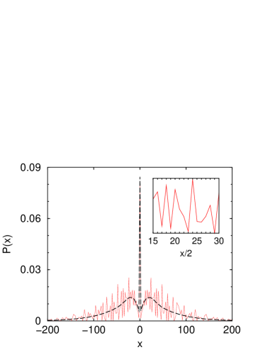
Figure 3: Probability distribution of the greedy random walk after $t=10^{2}$ steps. Shown are results for integer-valued step lengths (solid line) and continuum step lengths (dashed line). The latter distribution was scaled up by a factor 2. The inset shows detail of the prime-based fluctuations.

The probability distribution itself exhibits several intriguing features that lie outside of a scaling description (Fig. 3). First, there are huge fluctuations in the distribution. These arise because displacement values that are prime or have relatively few prime factors are hard to reach by a greedy random walk. While this variability in the distribution is striking, it does not play a role in the asymptotic scaling form of the distribution.

There is also a singularity at $x=0$ and secondary peaks at a distance $t^{1/2}$ from the origin. The singularity arises because the probability of being exactly at the origin is not affected by the enhancement mechanism of greedy walks. All that is required is an equal number of steps to the left and right, independent of when these steps occur. Thus the amplitude of this peak decays as $t^{-1/2}$, as in a pure random walk. In contrast, as follows from (13), the amplitude of the scaling part of the distribution scales as $t^{-1}$.

To visualize the envelope of the distribution and the anomalous behavior near the origin more clearly, we introduce a smoothed version of the greedy random walk in which the step length grows by an increment that is uniformly distributed between 0 and 2 upon each return to the origin. Such a construction still has a step length that equals, on average, the number of returns to the origin, but there are no longer any discreteness effects (Fig. 3). The resulting probability distribution clearly reveals secondary peaks close to the origin. These are due to walks that never return to the origin. For this class of walks, the contribution to the probability distribution in the continuum limit was given by Eq. (10). Since the characteristic length scale of this contribution is proportional to $t^{1/2}$, the secondary peaks get squeezed toward the origin when the distribution is plotted against the properly scaled coordinate $x/t$.

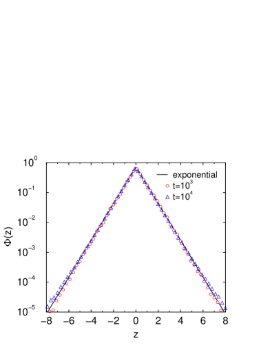
Figure 4: The scaling function of Eq. (3) for walks with $10^{3}$ and $10^{4}$ steps on a semi-logarithmic scale. Also shown as a reference is an exponential distribution. The distributions are normalized to have a unit rms displacement, $\langle z^{2}\rangle=1$.

More importantly, the continuum probability distribution of the greedy walk obeys scaling, with the scaling function a purely exponential function of the normalized displacement $z=x/x_{\rm rms}$, in agreement with our analytic prediction given in Eq. (14).

III Duration statistics

We now turn to the question that motivated this work, namely, how long does a game that is based on a greedy random walk last? More abstractly, how long does it take for a greedy random walk to escape the interval $[-L,L]$? Our basic result is that the typical escape time is relatively short, but higher moments still involve the diffusive time scale $L^{2}$.

The displacement scaling law (2) suggests that the typical escape time scales as

$$t\sim L^{\mu}$$ (17)

with $\mu=1/\nu=2/(\alpha+1)$. The exit-time distribution, $E(t,L)$, namely, the probability that the walk exits a system of size $L$ at time $t$, should then follow scaling in the large-$L$ limit (Fig. 5)

$$E(t,L)\sim L^{-\mu}\,\Psi\left(t\,L^{-\mu}\right).$$ (18)

Since $\mu<2$, the typical lifetime of a walk is shortened by the greedy walk mechanism.

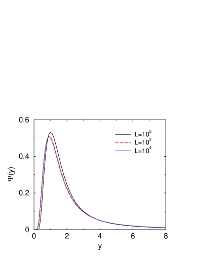
Figure 5: The scaling function of the exit-time distribution (Eq. (18)) from simulations with system size $L=10^{2}$ (solid line), $L=10^{3}$ (dashed line), and $L=10^{4}$ (dotted line).

The minimal escape time is realized by hybrid zig-zag/ballistic walks that have the maximal displacement. Similar to the considerations leading to Eq. (4), the escape time for such extremal walks is $t=\tau+L(\tau/2)^{-\alpha}$, with $\tau$ the duration of the zig-zag phase. The escape time is minimized when $\tau\sim L^{1/2\nu}\sim L^{\mu/2}$ and the minimal escape time also scales as $L^{\mu/2}$. Since the probability for such walks decays exponentially with the escape time, we then infer from Eq. (18), the asymptotic behavior

$$\Psi(y)\sim\exp(-1/y),$$ (19)

for $y\ll 1$. This scaling is independent of $\alpha$ and thus, is identical to that of an ordinary random walk. We conclude that short-lived games are relatively rare.

Long-lived walks are more interesting. To determine the likelihood of such walks, we need to understand greedy random walk trajectories (Fig. 2) in finer detail. First consider the return segments of the greedy walk. Upon the $j^{\rm th}$ return and after the next step, the walk is at $\pm j^{\alpha}$. Then from classic first-passage properties F68 ; fpp , the probability of returning again to the origin without escaping is $(1-j^{\alpha}/L)$, while the probability of escaping without another return is $j^{\alpha}/L$. Notice that the increase of the single-step length effectively reduces the system size by the step length. Using these results, the probability of returning to the origin at least $k$ times is

$$R_{k} = \left(1-\frac{1}{L}\right)\left(1-\frac{2^{\alpha}}{L}\right)\ldots\left(1-\frac{k^{\alpha}}{L}\right)$$ (20)

$$\sim \exp\left(-k^{1+\alpha}/L\right).$$

The typical number of returns to the origin before escape occurs is found from the criterion $R_{k}\approx 1/2$; this gives

$$k\sim L^{1/(1+\alpha)}.$$

This statement tell us the magnitude of the typical payoff in a greedy random walk-based game.

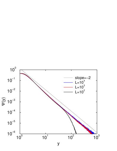
Figure 6: The scaling function of the exit-time distribution on a double logarithmic scale.

For a greedy walk to escape the system at time $t$, there may be $k\geq 0$ returns to the origin, followed by a non-return segment. From Eq. (20), the probability for the former event is $\exp\left(-k^{1+\alpha}/L\right)$. In the long-time limit, the probability for the non-return segment scales as $(\frac{k^{\alpha}}{L})^{3}\,\exp\left(-tk^{2\alpha}/L^{2}\right)$, where, as usual, we have ignored all factors of order one in the exponential. The exponential term is just the controlling factor for the escape probability of a random walk in an interval of length $L/k^{\alpha}$ fpp . The prefactor $(k^{\alpha}/L)^{3}$ ensures that the integral of this factor over all time gives the correct ultimate escape probability of $k^{\alpha}/L$. Putting these elements together, the probability $E(t,L)$ for a greedy walk to escape the interval $[-L,L]$ at time $t$ is

$$E(t,L)\sim\sum_{k=1}\left(\frac{k^{\alpha}}{L}\right)^{3}\,e^{-tk^{2\alpha}/L^{2}}\,\,e^{-k^{1+\alpha}/L}.$$ (21)

By converting the sum to an integral, and noting that in the long time limit, the last term is negligible, we obtain

$$E(t,L)\sim\frac{L^{1/\alpha}}{t^{3/2+1/2\alpha}},$$ (22)

over the intermediate time range $L^{\mu}\ll t\ll L^{2}$. Escape times larger that $L^{2}$ are realized by walks that never return to the origin. However, such walks are exponentially unlikely, $\exp(-t/L^{2})$, so that their contribution is irrelevant in the scaling limit. In the limit $\alpha\to\infty$, walks may return to the origin at most once, and the behavior $E(t,L)\sim t^{-3/2}$ follows from Eq. (10). Finally, the power-law form of $E(t,L)$ implies that the scaling function has the power-law decay for $y\gg 1$ (Fig. 6)

$$\Psi(y)\sim y^{-3/2-1/2\alpha}.$$ (23)

The existence of this power-law tail suggests that higher-order moments of the distribution are not characterized by the typical behavior (17). By integrating Eq. (22) up to the time scale $L^{2}$, we find three behaviors

$$\langle t^{n}\rangle\sim\begin{cases}L^{\mu\,n}&n<n_{c};\\ L\ln L&n=n_{c};\\ L^{2n-1}&n>n_{c}.\end{cases}$$ (24)

Low-order moments are characterized by the typical escape time, while high-order moments are described by pure diffusion. At the boundary $n_{c}=(\alpha+1)/2\alpha$, there is a logarithmic correction. Thus while the greedy walk mechanism significantly reduces the typical duration of the game, there are substantial fluctuations in this duration. In the worst case, the duration would be proportional to $L^{2}$, as in the ordinary random walk.

When the step length grows linearly with the number of returns to the origin, Eq. (22) shows that the exit time distribution has the asymptotic behavior $L/t^{2}$. Thus the average lifetime of a greedy walk includes the logarithmic correction

$$\langle t\rangle\propto L\ln L.$$ (25)

This behavior can be obtained directly by noticing that: (i) there are of the order $k\sim L^{1/2}$ returns, (ii) the average $k^{\rm th}$ return time is $\langle t_{k}\rangle\propto L+L/2+\cdots L/k\propto L\ln k$.

For completeness, we mention that the full survival probability can be computed via the Laplace transform. For an ordinary random walk starting at $x=1$ in a domain of length $L$ with absorbing boundary conditions, the Laplace transform of the first-passage probabilities at $x=0$ and $x=L$ are, respectively fpp ,

$$j_{-}(s) = \sinh[\sqrt{s/D}(L-1)]/\sinh[\sqrt{s/D}L]$$

$$j_{+}(s) = \sinh[\sqrt{s/D}]/\sinh[\sqrt{s/D}L].$$

The first-passage probability at $x=L$ for the greedy random walk is obtained by summing over the possible number of returns and scaling down the domain size by the step length $l_{k}$ at each return. This gives

$$E(s,L)=\sum_{k=0}^{\infty}\frac{\sinh\sqrt{s}}{\sinh[\sqrt{s}\frac{L}{l_{k}}]}\prod_{j=1}^{k}\frac{\sinh\left[\sqrt{s}\left(\frac{L}{l_{j}}-1\right)\right]}{\sinh[\sqrt{s}\frac{L}{l_{j}}]}.$$ (26)

The small-time and large-time behaviors given above follow from the large-$s$ and small-$s$ behaviors of this expression, respectively. Additionally, the $k$-th return probability given in Eq. (20) equals the $s\to 0$ limit of the product in Eq. (26).

IV Summary

The greedy random walk, in which the step length increases algebraically with the number of returns to the origin, exhibits a variety of unusual features. The distribution of displacements is non-Gaussian, despite the fact that each epoch is characterized by a Gaussian distribution. Similarly, the distribution of escape times decays as a power-law tail even though each segment has an ordinary exponential decay.

The most extended walks follow a two-stage process of immediate reversals followed by a ballistic trajectory. There are also several features of the probability distribution that are outside of scaling, including the contributions of walks that never return to the origin, walks that are exactly at the origin, and large prime-number-induced fluctuations.

The time for a greedy random walk to escape a finite interval is much smaller than that of ordinary random walks. However, because the distribution of escape times decays as a power law in the long time limit, there are large fluctuations in the escape time and the longest possible games have a similar length to those based on ordinary random walks.

We conclude that the greedy random walk provides a strategy for completing zero-sum games quickly. Increasing the stakes when the game is tied accelerates the path to richness or to ruin.

- (1) J. M. Hill and C. M. Gulati, J. App. Prob. 4, 931 (1981).
- (2) D. A. Levin, R. Pemantle, and Y. Peres, Ann. Prob. 29, 1637 (2001).
- (3) P. Diaconis and R. Durrett, J. Theo. Prob. 14, 899 (2001).
- (4) E. Ben-Naim and P.L. Krapivsky, Eur. Phys. J. B 25, 239 (2002).
- (5) D. Robinson and S. Vijay, Dreidel lasts Spins, math.CO/0403404.
- (6) W. Feller An Introduction to Probability Theory and Its Applications, (Wiley, New York, 1968).
- (7) G. H. Weiss, Aspects and Applications of the Random Walk, (North-Holland, Amsterdam, 1994).
- (8) S. Redner, A Guide to First-Passage Processes, (Cambridge University Press, New York, 2001).
- (9) J. Rudnick and G. Gaspari, Elements of the Random Walk: An Introduction for Advanced Students and Researchers, (Cambridge University Press, New York, 2004).
- (10) M. E. Fisher, J. Chem. Phys. 44, 616 (1966).
- (11) I. M. Lifshitz, S. A. Gredeskul, and L. A. Pastur, Introduction to the Theory of Disordered Systems (Wiley, New York, 1988).
- (12) M. Abramowitz and I. A. Stegun, Handbook of Mathematical Functions, (Dover, New York, 1972).
- (13) G. H. Weiss, and R. J. Rubin, Adv. Chem. Phys. 52, 363 (1983).