Effects of fluctuations and Coulomb interaction on the transition temperature of granular superconductors.

Abstract

We investigate the suppression of superconducting transition temperature in granular metallic systems due to (i) fluctuations of the order parameter (bosonic mechanism) and (ii) Coulomb repulsion (fermionic mechanism) assuming large tunneling conductance between the grains $g_{T}\gg 1$. We find the correction to the superconducting transition temperature for 3$d$ granular samples and films. We demonstrate that if the critical temperature $T_{c}>g_{T}\delta$, where $\delta$ is the mean level spacing in a single grain the bosonic mechanism is the dominant mechanism of the superconductivity suppression, while for critical temperatures $T_{c}<g_{T}\delta$ the suppression of superconductivity is due to the fermionic mechanism.

I Introduction

Being an experimentally accessible electronic system with the tunable parameters, Valles ; experiment ; Jaeger ; Simon ; Beloborodov99 ; Efetov02 granular superconductors, offer a unique testing ground for studying combined effects of disorder, Coulomb interactions and superconducting fluctuations that govern the physics of disordered superconductors and are central to mesoscopic physics. One of the fundamental questions long calling for investigation is the problem of suppression of the superconducting critical temperature, $T_{c}$, in granular superconductors and the role played in this suppression by the Coulomb repulsion and superconducting fluctuations. In this paper we present a quantitative theory of the suppression of $T_{c}$ in granular samples.

The customary belief was that - according to the Anderson theorem Anderson59 - disorder leaves critical temperature of a superconductor intact. However this result holds only in the mean field BCS approximation, and in all the cases where the extension beyond the BCS approximation is required, one can expect a noticeable suppression of the critical temperature.

The main mechanisms of the superconductivity suppression are Coulomb repulsion and superconducting fluctuations. For example, disorder shifts significantly the superconducting transition temperature in the $2d$ thin films Ovchinnikov73 ; Fukuyama81 ; Finkelstein87 ; Ishida98 ; Larkin99 . The physical reason for the suppression of the critical temperature is that in thin films the interaction amplitude in the superconducting channel decreases due to peculiar disorder-induced interference effects which enhance the effective Coulomb interaction. On the technical side, in order to evaluate the effect of disorder, one should sum a certain class of diagrams that include, in particular, cooperons and diffusons. In the subsequent discussion we will be referring to this mechanism of the superconductivity suppression as to the fermionic mechanism.

The superconducting transition temperature can also be reduced by the fluctuations of the order parameter, the effect being especially strong in low dimensions. The corresponding mechanism of the superconductivity suppression is called the bosonic mechanism. In particular, the bosonic mechanism can lead to the appearance of the insulating state at zero temperature. The physics of this state can be most easily understood in the case of a granular sample with weak intergranular coupling: the Cooper pair can be localized on a single grain if the charging energy is larger than the Josephson energy corresponding to the intergranular coupling Efetov80 . Later it was shown Fisher90 , that a similar mechanism of Cooper pair localization appears even in the case of the homogenously disordered films and the superconductor to insulator transition was predicted to occur at zero temperature.

In this paper we study the corrections to the superconducting transition temperature in granular metals perturbativelly. While this approach is restricted and cannot be used for study of non-perturbative effects such as the superconductor to insulator transition, it is useful in a sense that both relevant mechanisms of the critical temperature suppression can be studied systematically within the same framework. The power of the perturbative calculation in the study of granular metals was demonstrated in that it revealed an important energy scale $\Gamma=g_{\scriptscriptstyle T}\delta$, which was missed for example by the effective phase functional formalism, where $g_{\scriptscriptstyle T}$ is the tunneling conductance between the grains and $\delta$ is the mean energy level spacing for a single grain, appearing in granular materials. The presence of this energy scale which has a simple physical interpretation of an inverse average time that an electron spends in a single grain before tunneling to one of the neighboring grains Efetov , brings into play new behaviors that are absent in homogeneous media. In particular, the two different transport regimes at high, $T>\Gamma$, and low, $T<\Gamma$, temperatures appear. Lopatin03 In the high temperature regime the correction to the conductivity due to the Coulomb interaction depends logarithmically on temperature in all dimensions, while at low temperatures the interaction correction to conductivity has the Altshuler-Aronov form Altshuler and, thus is very sensitive to the dimensionality of the sample.

In a view of these findings one may expect that the correction to the superconducting transition temperature can also be different depending on whether the temperture is larger or smaller than the energy scale $\Gamma$.

In the present paper we analyze the mechanisms of the suppression of superconductivity in both temperature regimes. We find that the fermionic mechanism is temperature dependent and that its contribution is strongly reduced in the region $T>\Gamma$. In this regime the bosonic mechanism of the $T_{c}$ suppression becomes dominant. In the low temperature regime, $T<\Gamma$, the correction to the critical temperature is similar to that obtained for homogeneously disordered metals. In this regime the fermionic mechanism plays the major role as long as the intergranular tunneling conductance is large.

The paper is organized as follows: in Sec. II we summarize the results for the suppression of superconducting transition temperature of granular metals. In Sec. III we compare our results for the suppression of superconductivity in granular metals with known results for homogeneously disordered systems. In Sec. IV we introduce the model; the effect of fluctuations and Coulomb interaction on the superconducting transition temperature is then discussed in Sec. V. The mathematical details are relegated to the Appendixes.

II Summary of the results

It is convenient to discriminate corrections due to bosonic and fermionic mechanisms and write the result for the suppression $\Delta T_{c}$ of the superconductor transition temperature in a form

$${\frac{{\Delta T_{c}}}{{T_{c}}}}=\left({\frac{{\Delta T_{c}}}{{T_{c}}}}\right)_{b}+\left({\frac{{\Delta T_{c}}}{{T_{c}}}}\right)_{f},$$ (1a)

where the two terms in the right hand side correspond to the bosonic and fermionic mechanisms, respectively. The critical temperature $$T_{c}$$ in Eq. (1a) is the BCS critical temperature.

We find that at high temperatures, $T>\Gamma$, the fermionic correction to the superconducting transition temperature does not depend on the dimensionality of the sample

$$\left({\frac{{\Delta T_{c}}}{{T_{c}}}}\right)_{f}=-c_{1}\,\frac{\delta}{T_{c}},\hskip 22.76228ptd=2,3.$$ (1b)

where $c_{1}=7\zeta(3)/2\pi^{2}-(\ln 2)/4$ is the numerical coefficient and $d$ is the dimensionality of the array of the grains.

In the low temperature regime, $T<\Gamma$, the fermionic mechanism correction to the superconducting transition temperature depends on the dimensionality of the sample and is given by

$$\left(\frac{\Delta T_{c}}{T_{c}}\right)_{f}=-\left\{\begin{array}[]{lr}\frac{A}{2\pi\,g_{T}}\ln^{2}\frac{\Gamma}{T_{c}},\hskip 45.52458ptd=3&\\ \frac{1}{24\,\pi^{2}g_{T}}\ln^{3}\frac{\Gamma}{T_{c}},\hskip 36.98866ptd=2&\end{array}\right.,$$ (1c)

where $A=g_{T}a^{3}\int d^{3}q/(2\pi)^{3}\varepsilon_{\mathbf{q}}^{-1}\approx 0.253$ is the dimensionless constant, $a$ is the size of a single grain and

$$\varepsilon_{\mathbf{q}}=2g_{T}\sum_{\mathbf{a}}(1-\cos\mathbf{qa})$$ (1d)

with $\{\mathbf{a}\}$ being the lattice vectors (we consider a periodic cubic lattice of grains). Note that in the low temperature regime $T<\Gamma$ the correction to the critical temperature in the dimensionality $d=2$ coincides with that obtained for homogeneously disordered superconducting films upon the substitution $\Gamma\rightarrow\tau^{-1}$.

On the contrary, the correction to the transition temperature due to the bosonic mechanism in Eq. (1a) remains the same in both regimes and is given by

$$\left(\frac{\Delta T_{c}}{T_{c}}\right)_{b}=-\left\{\begin{array}[]{lr}\frac{14A\zeta(3)}{\pi^{3}}\;{\frac{1}{{g_{\scriptscriptstyle T}}}},\hskip 49.79231ptd=3&\\ {\frac{{7\zeta(3)}}{{2\pi^{4}g_{\scriptscriptstyle T}}}}\;\ln\frac{g_{\scriptscriptstyle T}^{2}\delta}{T_{c}},\hskip 39.83368ptd=2&\end{array}\right.,$$ (1e)

where $\zeta(x)$ is the zeta-function and the dimensionless constant $A$ was defined below Eq. (1c). Note that the energy scale $\Gamma$ does not appear in this bosonic part of the suppression of superconducting temperature in Eq. (1e). This stems from the fact that the characteristic length scale for the bosonic mechanism is the coherence length $\xi$ which is much larger than the size of a single grain. The result for the two dimensional case in Eq. (1e) is written with a logarithmic accuracy, assuming that $\ln(g_{\scriptscriptstyle T}^{2}\delta/T_{c})\gg 1$.

The above expression for the correction to the transition temperature due to the bosonic mechanism was obtained in the lowest order in the propagator of superconducting fluctuations and holds therefore as long as the value for the critical temperature shift given by Eq. (1e) is larger than the Ginzburg region $(\Delta T)_{\scriptscriptstyle G}$

$$(\Delta T)_{\scriptscriptstyle G}\sim\left\{\begin{array}[]{lr}\frac{1}{g_{\scriptscriptstyle T}^{2}}\frac{T_{c}^{2}}{g_{\scriptscriptstyle T}\delta}\hskip 39.83368ptd=3,&\\ \frac{T_{c}}{g_{\scriptscriptstyle T}}\hskip 56.9055ptd=2.&\end{array}\right.$$ (2)

Comparing the correction to the transition temperature $T_{c}$ given by Eq. (1e) with the width of the Ginzburg region, Eq. (2), one concludes that for $3d$ granular metals the perturbative result (1e) holds if

$$T_{c}<g_{\scriptscriptstyle T}^{2}\delta.$$ (3)

In two dimensions the correction to the transition temperature in Eq. (1e) is only logarithmically larger than $(\Delta T)_{G}$ in Eq. (2). With the logarithmic accuracy we note that the two dimensional result (1e) holds in the same temperature interval (3) as for the three dimensional samples.

Note that inside the Ginzburg region the higher order fluctuation corrections become important. Moreover, the non perturbative contributions, in particular, the contributions from superconducting vortices should be taken into account as well. These effects destroy the superconducting long range order and lead to Berezinskii-Kosterlitz-Thouless transition in $2d$ systems.

To summarize our results, we find that the correction to the superconducting transition temperature of granular metals comes from two different mechanisms; the dominant mechanism depends on temperature range.
(i) In the low temperature regime, $T<\Gamma$, the fermionic mechanism is the main mechanism of the suppression of $T_{c}$ and the correction to the transition temperature is given by Eq. (1c).
(ii) In the high temperature regime, $T>\Gamma$, the dominant mechanism is bosonic. At moderate temperatures, $T<g_{\scriptscriptstyle T}^{2}\delta$, the correction to the transition temperature is perturbative and is given by Eq. (1e), while at higher temperatures $T>g_{\scriptscriptstyle T}^{2}\delta$ the superconducting transition temperature must be determined by considering the critical fluctuations in the effective Ginzburg-Landau functional.

III Comparison of the suppression of superconductivity in granular and homogeneously disordered systems

In this section we compare our results for the suppression of superconductivity with the known results obtained for homogenously disordered superconductors. We begin our discussion with homogeneously disordered samples briefly reminding what is known about suppression of superconductivity in this case.

Both mechanisms of the suppression of superconductivity in homogeneously disordered films were discussed in several publications Ovchinnikov73 ; Fukuyama81 ; Finkelstein87 ; Fisher90 ; Ishida98 . In particular, for films with thickness $d$ such that $l\ll d\ll\xi$ where $l$ is the electron mean free path and $\xi$ is the coherence length it was shown that the result for the suppression of superconducting critical temperature can be written in analogous form with Eq. (1a), $\Delta T_{c}/T_{c}=(\Delta T_{c}/T_{c})_{f}+(\Delta T_{c}/T_{c})_{b}$, where Ovchinnikov73

$$\left(\frac{\Delta T_{c}}{T_{c}}\right)_{f}=-\frac{1}{24\,\pi^{2}g}\ln^{3}[1/(\tau T_{c})],$$ (4a)

and

$$\left(\frac{\Delta T_{c}}{T_{c}}\right)_{b}=-\frac{7\zeta(3)}{2\pi^{4}g}\ln[g/(\tau T_{c})].$$ (4b)

Here $g\gg 1$ is the film conductance (per one spin component) and $\tau$ is the elastic electron mean free time. One can see from Eqs. (4) that in the regime of large conductance within the logarithmic accuracy the fermionic mechanism is the dominant one. At the same time, if the conductance is not too large both corrections become of the order of one and the bosonic mechanism becomes very important as well. In this regime the suppression of superconductivity should be considered non-perturbativelly as in Ref. Fisher90, for the bosonic mechanism and in Ref. Finkelstein87, for the fermionic mechanism.

In granular superconductors situation is different due to appearance of the energy scale $\Gamma=g_{\scriptscriptstyle T}\delta$. As one can see from Eqs. (1) both mechanisms of the suppression of superconductivity are important. In the limit of high temperatures $T>\Gamma$ the interference effects in granular metals are suppressed and that is why the fermionic mechanism is strongly reduced, Eq. (1b). The shift of the superconducting critical temperature in this region is defined by the bosonic mechanism and has a classic origin. In the low temperature limit $T<\Gamma$ quantum interference effects become important therefore the suppression of superconductivity is defined by the fermionic mechanism. The fact that in the low temperature regime the correction to the superconducting transition temperature for a granular samples can be obtained from the corresponding result for the homogenously disordered samples via the substitution of the effective diffusion coefficient $D=g_{T}\delta a^{2}$, suggests that the universal low temperature description proposed in Ref. Universal, can be generalized to include the superconducting channel.

IV The model

Now we turn to the quantitative description of our model and derivation of Eqs. (1a, 1c, 1e). We consider a $d-$dimensional array of superconducting grains in the metallic state. The motion of electrons inside the grains is diffusive and they can tunnel between grains. We assume that if the Coulomb interaction were absent, the sample would have been a good metal at $T>T_{c}$.

The Hamiltonian of the system of the coupled superconducting grains is:

$$\hat{H}=\hat{H}_{0}+\hat{H}_{c}+\hat{H}_{t}.$$ (5a)

The term $$\hat{H}_{0}$$ in Eq. (5a) describes isolated disordered grains with an electron-phonon interaction

$$\hat{H}_{0}=\sum\limits_{i,k}\epsilon_{i,k}a_{i,k}^{\dagger}a_{i,k}-\lambda\sum\limits_{i,k,k^{\prime}}a_{i,k}^{\dagger}a_{i,-k}^{\dagger}a_{i,-k^{\prime}}a_{i,k^{\prime}}+\hat{H}_{imp},$$ (5b)

where $$i k\equiv(\mathbf{k},\uparrow) -k\equiv(-\mathbf{k},\downarrow) \lambda>0 a_{i,k}^{\dagger}(a_{i,k}) k i \hat{H}_{imp} \hat{H}_{c}$$ labels the grains, , ; is the interaction constant; are the creation (annihilation) operators for an electron in the state of the -th grain, and represents the elastic interaction of the electrons with impurities. The term in Eq. (5a) describes the Coulomb repulsion both inside and between the grains and is given by

$$\hat{H}_{c}={\frac{{\ e^{2}}}{{\ 2}}}\,\sum_{ij}\,\hat{n}_{i}\,C_{ij}^{-1}\,\hat{n}_{j},$$ (5c)

where $$C_{ij} \hat{n}_{i} i$$ is the capacitance matrix and is the operator of the electron number in the -th grain.

Eq. (5c) describes the long range part of the Coulomb interaction, which is simply the charging energy of the grains. The last term in the right hand side of Eq. (5a) is the tunneling Hamiltonian

$$\hat{H}_{t}=\sum_{ij,p,q}t_{ij}a_{i,p}^{\dagger}a_{j,q},$$ (5d)

where $t_{ij}$ is the tunneling matrix element corresponding to the points of contact of $i$-th and $j-$th grains and $p$, $q$ stand for the states in the grains.

In the following section we will study effects of fluctuations on the superconducting transition temperature of granular metals based on the model defined by Eqs. (5).

V Effects of fluctuations and Coulomb interaction on transition temperature

The superconducting transition temperature can be found by considering corrections to the anomalous Green function $F$ due to fluctuations of the order parameter and Coulomb interaction in the presence of infinitesimal source of pairs $\Delta$. Ovchinnikov73 Without account of fluctuations and interaction effects, the anomalous Green function $F$ is given by the expression AGD

$$F(\xi,\varepsilon_{n})=\Delta/(\varepsilon_{n}^{2}+\xi^{2}),$$ (6)

where $\xi=\mathbf{p}^{2}/2m-\mu,$ and $\varepsilon_{n}=2\pi T(n+1/2)$ is the fermionic Matsubara frequency. The suppression of the transition temperature $T_{c}$ is determined by the correction to the function $F(\xi,\varepsilon_{n})$

$$\frac{\Delta T_{c}}{T_{c}}={\frac{T}{\Delta}}\,\int d\xi\,\sum\limits_{\varepsilon_{n}}\delta F(\xi,\varepsilon_{n}),$$ (7)

where the function $\delta F(\xi,\varepsilon_{n})$ represents the leading order corrections to the anomalous Green function $F(\xi,\varepsilon_{n})$ due to pair density fluctuations and Coulomb interaction.

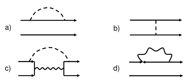
Figure 1: Diagrams a) - c) describe the correction to the superconducting transition temperature due to Coulomb repulsion. The diagram d) describes correction to the transition temperature due to superconducting fluctuations. All diagrams are shown before averaging over the impurities. The solid lines denote the electron propagators, the dashed lines describe screened Coulomb interaction and the wavy lines describe the propagator of superconducting fluctuations.

The function $\delta F(\xi,\varepsilon_{n})$ can be found by means of two different methods which lead to identical results: (i) solving the Usadel equation with the help of perturbation theory in powers of the fluctuating order parameter and potential and further averaging over them using the Gaussian approximation Ovchinnikov73 or (ii) using the diagrammatic technique. For our purpose we choose the diagrammatic approach. All diagrams (before impurity averaging) which contribute to the suppression of the transition temperature in Eq. 7 are shown in Fig. 1. One can see that there exist two qualitatively different classes of diagrams. First, the diagrams a) - c) describe corrections to the transition temperature due to Coulomb repulsion and represent the so called fermionic mechanism of the suppression of superconductivity. The second type, diagram d), describes a correction to the transition temperature due to superconducting fluctuations and represents the bosonic mechanism. It may seem surprising that we classify the diagram (c) as belonging to the fermionic mechanism, since this diagram contains both Coulomb and Cooper pair propagators. The reason is that, as we will show below (see also Ref. Finkelstain_review, ), there are dramatic cancellations between contributions of diagrams of the types (a,b) and (c). It is this cancellation that is responsible for the smallness of the contribution of the fermionic mechanism at high temperatures $T>\Gamma$. The diagrams of type (c) were not taken into account in Ref. BLV_2004, , where a different result for the suppression of the transition temperature was obtained Aleiner . In what follows we consider both mechanisms of the suppression of superconductivity in details.

V.1 Suppression of superconductivity due to fluctuations of the order parameter: bosonic mechanism

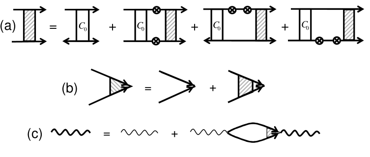
Figure 2: Diagrams (a) define the Cooperon propagator (shaded rectangle), Eq. (8), in terms of the single grain Cooperon $C_{0}.$ Diagrams (b) describe the renormalization of the BCS interaction vertex due to impurities. The superconducting propagator, Eq. (9), is represented by the thick wavy line and is defined by the diagrams (c) where the thin wavy line denotes the bare superconducting propagator. The solid lines denote the propagator of electrons and the tunneling vertices are denoted as the circles.

In this section we consider the suppression of the superconducting transition temperature in granular metals due to fluctuations of the order parameter (bosonic mechanism). We will use the diagrammatic technique developed in Refs. Beloborodov99, ; Efetov, . The main building block of the diagrams that will be considered in this section is the Cooperon propagator defined by the diagrams shown in Fig. 2 a. In the regime under consideration all characteristic energies are much less than the Thouless energy $E_{\scriptscriptstyle T}=D/a^{2},$ where $D$ is the diffusion coefficient. This allows us to use the zero dimensional approximation for a single grain Cooperon propagator $C_{0}^{-1}=\tau|\Omega_{n}|$. The resulting expression for the Cooperon is

$$C(\Omega_{n},\mathbf{q})=\tau^{-1}(|\Omega_{n}|+\varepsilon_{\mathbf{q}}\delta)^{-1},$$ (8)

where $\mathbf{q}$ is the quasi-momentum and $\Omega_{n}$ is the bosonic Matsubara frequency. The parameter $\varepsilon_{\mathbf{q}}$ in the right hand side of Eq. (8) appears due to the electron tunneling from grain to grain, it was defined in Eq. (1d).

The propagator of superconducting fluctuations, $K(\Omega_{n}\mathbf{q})$ is defined by the diagrams shown in Fig. 2 b and c. They result in the following expression

$$K(\Omega_{n},\mathbf{q})=\left[\ln\frac{T}{T_{c}}+\psi\left(\frac{1}{2}+\frac{|\Omega_{n}|+\varepsilon_{\mathbf{q}}\delta}{4\pi T}\right)-\psi\left(\frac{1}{2}\right)\right]^{-1},$$ (9)

with $\psi(x)$ being the digamma function.

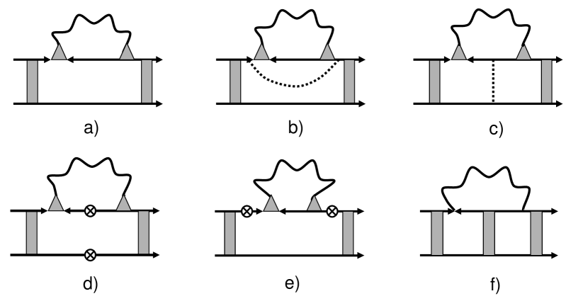
Figure 3: Diagrams describing correction to the transition temperature due to superconducting fluctuations (bosonic mechanism). The diagrams were obtained after averaging the diagram d) in Fig. 1 over the disorder. The solid lines denote the propagator of electrons, the dotted lines describe the elastic interaction of electrons with impurities and the wavy lines describe the propagator of superconducting fluctuations. The shaded rectangle and triangle denote the Cooperon, see Eq. (8), and impurity vertex of granular metals respectively. The tunneling vertices are denoted as the circles.

The diagrams describing the correction to the transition temperature in the lowest order with respect to the superconducting fluctuation propagator $K(\Omega_{n},\mathbf{q})$ are shown in Fig. 3.

Deriving the analytical result for the diagrams in Fig. 3 it is important to take into account the fact that the single electron propagator itself gets renormalized due to electron hopping. Tunneling processes give rise to an additional term in the self-energy part of the single electron propagator, see Fig. 4

$$\tau^{-1}=\tau_{0}^{-1}+2dg_{T}\delta,$$ (10)

where $\tau_{0}$ is the unrenormalized electron mean free time. Although the second term in the right hand side of Eq. (10) is much smaller than the first one, it is important to keep it because the leading order contribution in $\tau_{0}^{-1}$ to the correction to superconducting transition temperature cancels.

The contribution of each diagram in Fig. 3 to the suppression of superconducting critical temperature is presented in Appendix A. Here we write the final expression for the contribution of the diagrams (a)-(f) in Fig. 3 to the superconducting transition temperature

$$\left(\frac{\Delta T_{c}}{T_{c}}\right)_{b}=-\pi T^{2}\delta\sum\limits_{{\bf q}}\left[\sum\limits_{\varepsilon_{n}(\varepsilon_{n}-\Omega_{n})>0}\frac{K(\Omega_{n},{\bf q})[2|\varepsilon_{n}|+|2\varepsilon_{n}-\Omega_{n}|+\varepsilon_{\bf q}\delta]}{\varepsilon_{n}^{2}(|2\varepsilon_{n}-\Omega_{n}|+\varepsilon_{\bf q}\delta)^{2}}-\sum\limits_{\varepsilon_{n}(\varepsilon_{n}-\Omega_{n})<0}\frac{K(\Omega_{n},{\bf q})}{\varepsilon_{n}^{2}(|\Omega_{n}|+\varepsilon_{\bf q}\delta)}\right].\hskip 28.45274pt$$ (11)

Here the summation is going over the quasi-momentum, $\mathbf{q}$ and over the fermionic, $\varepsilon_{n}=\pi T(2n+1)$ and bosonic, $\Omega_{n}=2\pi Tn$ Matsubara frequencies.

The main contribution to the suppression of superconducting transition temperature in Eq. (11) comes from the region of classical fluctuations and is given by the term with $\Omega_{n}=0$. Performing summation over the fermionic Matsubara frequency $\varepsilon_{n}$ in Eq. (11) we obtain the following result

$$\left(\frac{\Delta T_{c}}{T_{c}}\right)_{b}=-\frac{14\zeta(3)}{\pi^{3}}\sum\limits_{\mathbf{q}}\frac{1}{\varepsilon_{\mathbf{q}}},$$ (12)

where $\zeta(x)$ is the zeta-function. Equation (12) for the suppression of superconducting transition temperature is valid outside the Ginzburg region otherwise the lowest order approximation in the superconducting propagator which we used to derive Eq. (12) is not justified. Performing summation over the quasi-momentum $\mathbf{q}$ in Eq. (12) we obtain the final result for the suppression of superconductivity due to the bosonic mechanism, Eq. (1e ). The singularity in two dimensional case should be cut at momenta $\mathbf{q}_{min}^{2}=a^{-2}\,(T_{c}/g_{T}^{2}\delta)$ in accordance with the expression for the Ginzburg number

$$Gi\sim\left\{\begin{array}[]{lr}\frac{1}{g_{T}}\hskip 42.67912pt2d,&\\ \frac{1}{g_{T}^{2}}\frac{T_{c}}{g_{T}\delta}\hskip 28.45274pt3d.&\end{array}\right.$$ (13)

The divergence of the correction to the transition temperature in $2d$, Eq. (12), means that flucutuations destroy the superconducting long range order, which is to be recovered by introducing the artificial cutoff ${\bf q}_{\min}$. Then the critical temperature which we calculate should be viewed as a crossover temperature rather than the temperature of a true phase transition. However, since experimentally such a temperature marks a sharp decay of the resistivity, the notion of the transition temperature still makes a perfect sense.

It follows from Eq. (13) that for $3d$ granular metals the Ginzburg number is small in comparison with the right hand side of Eq. (12) and the Gaussian approximation for bosonic mechanism is justified for temperatures $T_{c}<g_{\scriptscriptstyle T}^{2}\delta$. In $2d$ case the result (12) holds with the logarithmic accuracy in the same temperature interval $g_{\scriptscriptstyle T}^{2}\delta>>T_{c}$.

The correction to the transition temperature, Eq. (12), can be interpreted as a contribution of the fluctuations of the superconducting order parameter. These fluctuations can be considered as a virtual creation of Cooper pairs which are bosons. That is why we call this mechanism of the suppression of the superconductivity bosonic. The correction $\Delta T_{c}$, can be rather easily obtained via the Ginzburg-Landau expansion in the order parameter $\Delta\left(\mathbf{r}\right)$ near the critical temperature. For the granular system the free energy functional $F\left[\Delta\right]$ can be written as follows

$$F=\sum_{i}\left[\frac{\tilde{\tau}}{\delta}\left|\Delta_{i}\right|^{2}+\frac{b}{2}\left|\Delta_{i}\right|^{4}\right]+\sum_{i,j}J_{ij}\left|\Delta_{i}-\Delta_{j}\right|^{2},$$ (14a)

where the coefficients $$\tilde{\tau} b$$ and are given by

$$\tilde{\tau}=\frac{T-T_{c}}{T_{c}},\hskip 8.5359ptb={{7\zeta(3)}\over{8\,\pi^{2}T_{c}^{2}\delta}},$$ (14b)

with $J_{i,i\pm 1}=J_{0}=\pi g_{T}/16\,T_{c}$ being the Josephson coupling between the grains. Neglecting the quartic term in Eq. (14a) we obtain the propagator of $\left\langle\Delta_{\bf q}\Delta_{-\bf q}\right\rangle_{0}$ in the form

$$\left\langle\Delta_{\bf q}\Delta_{-\bf q}\right\rangle_{0}=\frac{T_{c}\delta}{\tilde{\tau}+(\pi\delta/8T_{c})\,\varepsilon_{\mathbf{q}}}.$$ (15)

The correction to the transition temperature can be found by calculating the first order in $b$ contribution to the self energy $\Sigma^{\left(1\right)}$:

$$\Sigma^{\left(1\right)}=2b\sum_{\bf q}{\delta\over{\tilde{\tau}+(\pi\delta/8T_{c})\varepsilon_{\mathbf{q}}}}.$$ (16)

This correction renormalizes the critical temperature. Putting $\tilde{\tau}=0$ in Eq. (16) we come to the result expressed by Eq. (12).

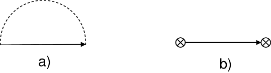
Figure 4: Diagrams describing self-energy corrections to the single electron propagator due to a) elastic interaction of electrons with impurities and b) electron hopping. The solid lines denote the bare propagator of electrons and the doted line describes the elastic interaction of electrons with impurities. The tunneling vertices are described by the circles.

The fermionic mechanism of the suppression of the superconductivity is more complicated and we consider it in the next section.

V.2 Suppression of superconductivity due to Coulomb repulsion: fermionic mechanism

In this section we consider the suppression of the superconducting transition temperature in granular metals due to combine effects of Coulomb interaction and disorder (fermionic mechanism). The Coulomb interaction in granular metals is screened by surrounding electrons as in any metal. The diagrams that describe the screened effect are presented in Fig. 5. The diagrams (a) define the diffusion propagator in granular metals. As in the case with the Cooperon, Eq. (8), we can consider the single grain Diffusion in the zero dimensional approximation such that $D_{0}^{-1}=\tau|\Omega_{n}|$ and for the diffusion propagator we obtain the expression

$$D(\Omega_{n},\mathbf{q})=\tau^{-1}(|\Omega_{n}|+\varepsilon_{\mathbf{q}}\delta)^{-1},$$ (17)

that coincides with the Cooperon propagator in Eq. (8). The diagram (b) in Fig. 5 describes the renormalization of the Coulomb vertex due to impurities and the diagram (c) defines the screened Coulomb interaction

$$V(\Omega_{n},{\bf q})=\left[{{C({\bf q})}\over{e^{2}}}+{{2\varepsilon_{\bf q}}\over{|\Omega_{n}|+\varepsilon_{\bf q}\delta}}\right]^{-1},$$ (18)

where $C(\bf q)$ is the Fourie transform of the capacitance matrix which has the following asymptotic form at $q\ll a^{-1}$

$$C^{-1}(\mathbf{q})=\frac{2}{a^{d}}\,\left\{\begin{array}[]{rl}&\pi/q\hskip 39.83368ptd=2,\\ &2\pi/q^{2}\hskip 31.2982ptd=3.\end{array}\right.$$ (19)

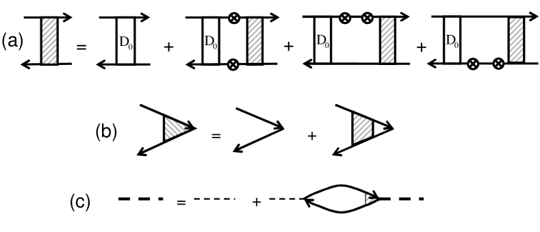
Figure 5: Diagrams (a) define the Diffusion propagator $D(\Omega_{n},{\bf q})$, Eq. (17), in terms of the single grain diffusion propagator $D_{0}(\Omega_{n}).$ Diagrams (b) define the renormalization of the Coulomb vertex due to impurity scattering. Diagrams (c) define the dynamically screened Coulomb interaction, Eq. (18). The thin dashed lines represent the bare Coulomb interaction while the thick lines denote the screened Coulomb interaction.

The correction to the critical temperature due to Coulomb interaction before averaging over impurities is given by the diagrams a-c in Fig 1. Averaging over the impurities leads to rather complicated formulae. We will consider the contributions from the diagrams a,b and c separately presenting the total correction to the critical temperature due to Coulomb interaction as

$$\left(\frac{\Delta T_{c}}{T_{c}}\right)_{f}=\langle X_{1}\rangle+\langle X_{2}\rangle,$$ (20)

where the term $X_{1}$ represents the contribution of the diagrams a and b in Fig. 1 while $X_{2}$ represents the contribution of the diagram c and $\langle...\rangle$ means averaging over the disorder. The two terms in the right hand side of Eq. (20) have a transparent physical meaning: the term $X_{1}$ describes the renormalization of the Cooperon due to Coulomb repulsion while the term $X_{2}$ describes the vertex renormalization. After the disorder averaging the terms $\langle X_{1}\rangle$ and $\langle X_{2}\rangle$ are represented in Figs. 6 and 7, respectively. The evaluation these diagrams is presented in Appendix B. The final expression for the correction to the critical temperature due to the fermionic mechanism has the following form

$$\left(\frac{\Delta T_{c}}{T_{c}}\right)_{f} = -4T\sum_{{\bf q},\Omega_{n}>0}V(\Omega_{n},{\bf q})\left[F(\Omega_{n})\,{{\varepsilon_{\bf q}\delta}\over{(\Omega_{n}+\varepsilon_{\bf q}\delta)^{2}\Omega_{n}}}+{1\over{4\pi T}}\,{{\varepsilon_{\bf q}\delta}\over{\Omega_{n}^{2}-(\varepsilon_{\bf q}\delta)^{2}}}\,\psi^{\prime}\left(\frac{1}{2}+\frac{\Omega_{n}}{2\pi T}\right)\right.$$ (21a)

$$+ \left.2F(\Omega_{n})\,K(\Omega_{n},{\bf q})\,{{(\varepsilon_{\bf q}\delta)^{2}}\over{[\Omega_{n}^{2}-(\varepsilon_{\bf q}\delta)^{2}]^{2}}}\,\left(\psi[\,1/2+(\Omega_{n}+\varepsilon_{\bf q}\delta)/4\pi T\,]-\psi[\,1/2+\Omega_{n}/2\pi T\,]\right)\right],$$

where we introduced the notation

$$F(\Omega_{n})=\psi(1/2+\Omega_{n}/2\pi T)-\psi(1/2),$$ (21b)

and the propagator $$K(\Omega_{n},{\bf q}) \mathbf{q} \Omega_{n}. V(\Omega_{n},\mathbf{q}) E_{c} \delta$$ was defined in Eq. (9). The summation in Eq. (21a) is going over the quasi-momentum and the bosonic Matsubara frequencies The propagator of the screened electron-electron interaction, , Eq. (18), in the limit when the charging energy, , is much larger than the average mean level spacing, , can we written as

$$V(\Omega_{n},\mathbf{q})={\frac{{2E_{C}(\mathbf{q})(|\Omega_{n}|+\varepsilon_{\mathbf{q}}\delta)}}{{4\varepsilon_{\mathbf{q}}E_{C}(\mathbf{q})+|\Omega_{n}|}}}.$$ (21c)

where $E_{C}(\mathbf{q})=e^{2}/2C(\mathbf{q})$ is the charging energy.

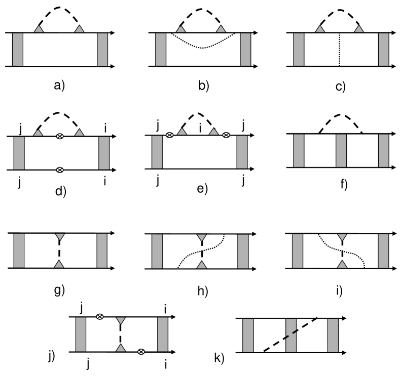
Figure 6: Diagrams obtained from diagrams a and b in Fig. 1 after disorder averaging. The solid lines denote the propagator of electrons, the dashed lines describe screened Coulomb interaction and the dashed-dot lines describe the elastic interaction of electrons with impurities. The shaded rectangle and triangle denote the renormalized Cooperon, see Eq. (8), and impurity vertex of granular metals respectively. The indices $i$ and $j$ stand for the grain numbers. The tunneling vertices are described by the circles.

An important feature of Eq. (21a) is that the expression in the big square brackets in the right hand side vanishes at ${\bf q}\to 0$ for any frequency $\Omega_{n}.$ This is due to the fact that the potential $V(\Omega_{n},{\bf q}=0)$ represents a pure gauge and thus it should not contribute to the thermodynamic quantities such as the superconducting critical temperature. As a consequence one can see that the contribution of the frequencies $\Omega_{n}$ that belong to the interval

$$\varepsilon_{\bf q}\delta<\Omega_{n}<\varepsilon_{\bf q}E_{C}({\bf q})$$ (22)

have a small contribution to the critical temperature correction given by Eq. (21a), Finkelstain_review . For this reason we do not expect the Coulomb energy $E_{C}$ to appear in the final result. At the same time the frequencies $\Omega_{n}$ that belong to the interval (22) are fully responsible for the logarithmic renormalization of the integranular conductance $g_{\scriptscriptstyle T}(T)=g_{\scriptscriptstyle T}-(1/2\pi d)\,\ln(g_{T}E_{\scriptscriptstyle C}/T)$, where the Coulomb energy explicitly appears in the result.

The expression in the r.h.s. of Eq. (21a) is quite complicated; we cannot derive a simple result at any arbitrary temperature. Further on we will consider only the limiting cases $T>\Gamma$ and $T<\Gamma$ where the calculations are considerably simplified.

If the temperature $T$ is sufficiently small, $T\ll\Gamma$, the summation over the Matsubara frequencies can be replaced with the integral. One can easily see that the singularities at $\Omega=\varepsilon_{\bf q}\delta$ in the second and third terms in Eq. (21a) cancel each other. Their appearance, in fact, is a pure artifact of the representation of the result in terms of the $\psi-$functions. With logarithmic accuracy one can leave only the first term in Eq. (21a); this results in

$$\left(\frac{\Delta T_{c}}{T_{c}}\right)_{f}=-{1\over{2\pi}}\sum_{\bf q}{1\over{\varepsilon_{\bf q}}}\,\ln^{2}{{\varepsilon_{\bf q}\delta}\over{T}},\;\;\;\;\varepsilon_{\bf q}\delta\gg T.$$ (23)

In the $3d$ case one can neglect the $q-$ dependence under the logarithm in Eq. (23), and the summation over quasimomentum leads to the logarithmically accurate final result (1c). In two dimensions, the main contribution in summation over quasimomentum in Eq. (23) comes from the low momenta $q\ll 1/a$ where the energy $\varepsilon_{\bf{q}}$ can be written as $\varepsilon_{\bf{q}}=g_{T}{\bf q}^{2}a^{2}$, and the granular system becomes equivalent to a homogenously disordered one. Summation over $q$ with the logarithmic accuracy leads to the final result  (1c) for 2D case. No wonder that the result, Eq. (1c) in 2D agrees with the known result for disorder metals Refs. Ovchinnikov73, ; Fukuyama81, ; Finkelstein87, ; Finkelstain_review, . Equation (1c) in the 2D case has a universal form and is expressed in terms of the tunneling conductance $g_{\scriptscriptstyle T}$ and the effective relaxation time $\left(g_{\scriptscriptstyle T}\delta\right)^{-1}$. For the homogenously disordered samples the latter time should be replaced by the elastic scattering time $\tau$.

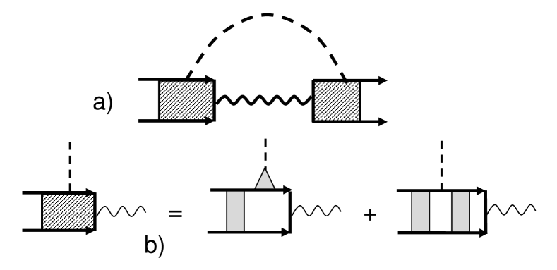
Figure 7: Diagrams describing vertex renormalization obtained from the diagram c) in Fig. 1 after averaging over the disorder. All notations are the same as in Figs. 2 and 4.

In the opposite limit, $T\gg\Gamma$ the quantity $\varepsilon_{\bf q}\delta$ can be neglected with respect to the Matsubara frequencies $\Omega_{n}$ and the result is drastically different from the one given by Eq. (1c). The potential $V(\Omega_{n},{\bf q})$ in this limit takes the form $V(\Omega_{n},{\bf q})=|\Omega_{n}|/2\varepsilon_{\bf q}$ such that $\varepsilon_{\bf q}$ cancels in the main approximation. Summation over Matsubara frequencies then leads to the correction Eq. (1b).

One thus can see from the above that in the limit $T\gg\Gamma$ the fermionic mechanism of the suppression of the superconductivity is no longer efficient. This can be seen rather easily in another way using the phase approach of Ref. Efetov02, . Following these works one decouples the Coulomb interaction, Eq. (5c) by integration over a phase $\phi$

$$\exp\left(-\frac{e^{2}}{2}\int d\tau\sum_{ij}{n}_{i}(\tau)C_{ij}^{-1}{n}_{j}(\tau)\right) = \int\exp\left(-i\sum_{i}\int n_{i}(\tau)\dot{\phi}_{i}\left(\tau\right)d\tau-\sum_{ij}\int d\tau\dot{\phi}_{i}\left(\tau\right)\frac{C_{ij}}{2e^{2}}\dot{\phi}_{j}\left(\tau\right)\right)D\phi,$$ (24)

where $n_{i}(\tau)=\int\psi^{\ast}\left(\mathbf{r}_{\mathbf{i}},\tau\right)\psi\left(\mathbf{r}_{i},\tau\right)d\mathbf{r}_{i}$ is the electron number in the i-th grain and $\psi$ are fermionic fields. With this decoupling the variable $\dot{\phi}$ plays a role of an additional chemical potential. In the limit $T\gg\Gamma$ (and only in this limit) the phase $\phi$ can be gauged out via the replacement

$$\psi\left(\mathbf{r}_{i},\tau\right)\rightarrow\psi\left(\mathbf{r}_{i},\tau\right)\exp\left[-i\phi_{i}\left(\tau\right)\right].$$ (25)

Substituting Eq. (25) into Eq. (5a - 5d) (or to be more precise, into the corresponding Lagrangian in the functional integral representation) we immediately see that the phase $\phi$ enters the tunneling term, Eq. (5d) only. However, this term is not important in the limit $T\gg\Gamma$ and we conclude that the long range part of the Coulomb interaction leading to charging of the grains is completely removed. Therefore, the effect of the Coulomb interaction on the superconducting transition temperature must be small and this is seen from Eq. (1b). This conclusion matches well the fact that the upper limit in the logarithms in Eq. (1c) is just $\Gamma$ and at temperatures exceeding this energy the logarithms should disappear. At low temperatures $T<\Gamma$ the phase description does not apply and the non-trivial result, Eq. (1c), appears. This result is of the pure quantum origin, and interference effects are very important. In the limit of high temperatures $T>\Gamma$ the interference effects are suppressed, that is why the fermionic mechanism of the suppression of the superconductivity is no longer efficient.

VI Discussion

We have described the suppression of the superconducting transition temperature due to (i) fluctuations of the order parameter (bosonic mechanism) and (ii) Coulomb repulsion (fermionic mechanism) in granular metallic systems at large tunneling conductance between the grains, $g_{\scriptscriptstyle T}\gg 1$. We have calculated the correction to the transition temperature for $3d$ granular samples and films. We have demonstrated that at temperature $T>g_{\scriptscriptstyle T}\delta$ the suppression of superconductivity in granular metals is determined by the bosonic mechanism while at low temperatures, $T<g_{\scriptscriptstyle T}\delta$, the suppression of superconductivity is dominated by the fermionic mechanism.

The bosonic mechanism has a classical origin. The fermionic mechanism is of the quantum origin and is relevant at low temperature $T<\Gamma$ where quantum interference effects are pronounced. In the opposite limit $T>\Gamma$ the coherence is lost and the fermionic mechanism of suppression of the conductivity is no longer efficient. Thus the classical bosonic mechanism is more important at high temperatures, whereas the quantum fermionic one is efficient at low temperatures.

The results of the theoretical study presented in this paper can be checked experimentally. Apparently, the best way to do this is to study the dependence of the superconducting transition temperature $T_{c}$ of granular metals as a function of the tunneling conductance $g_{\scriptscriptstyle T}$. Practically this can be done by studying several granular samples with different tunneling conductances (different oxidation coating). The experimental curves for $T_{c}$ suppression should have a different slope at high $T_{c}>g_{\scriptscriptstyle T}\delta$ and low $T_{c}<g_{\scriptscriptstyle T}\delta$ critical temperatures due to the fact that the suppression of the superconductivity is given by the two different mechanisms. Moreover, the difference between the dependence of the critical temperature on the tunneling conductance $T_{c}(g_{\scriptscriptstyle T})$ in granular and homogeneously disordered systems can give an information on the morphology of the sample, i.e. answer the question whether the samples are homogeneously disordered or granular.

Another interesting consequence of our results in Eqs. (1) is the following: since at low critical temperatures $T_{c}<g_{\scriptscriptstyle T}\delta$ the suppression of superconductivity in granular metals is given by the fermionic mechanism and upon the substitution $g_{\scriptscriptstyle T}\delta\rightarrow\tau^{-1}$ it coincides with the proper result for homogeneously disordered samples, Ovchinnikov73 one can generalize the renormalization group result by Finkelstein Finkelstein87 for the $T_{c}$ suppression. The latter result obtained for homogeneously disordered films can be applied to the case of the granular superconductors upon the proper substitution for the diffusion coefficient $D=g_{\scriptscriptstyle T}\delta a^{2}$, where $a$ is the size of a single grain.

Appendix A Evaluation of diagrams for the bosonic mechanism

In this appendix we evaluate diagrams for bosonic mechanism presented in Fig. 3 beginning with consideration of the diagrams a), b) and c). These three diagrams can be conveniently combined in a single diagram introducing the Hikami box Hikami81 as it is shown in Fig. 8. For zero dimensional grain (all characteristic energies are much less than the Thouless energy) Hikami box is given by the following expression

$$H(\varepsilon_{n_{1}},\varepsilon_{n_{2}},\varepsilon_{n_{3}},\varepsilon_{n_{4}})=2\pi\tau^{2}(|\varepsilon_{n_{1}}|+|\varepsilon_{n_{2}}|+|\varepsilon_{n_{3}}|+|\varepsilon_{n_{4}}|),$$ (26)

where $\varepsilon_{n_{i}}$ are fermionic Matsubara frequencies. Using Eq. (26) and evaluating the diagram shown in Fig. 6b we obtain the following result for the sum of these three diagrams

$$-\pi T^{2}\delta\sum\limits_{\varepsilon_{n}(\varepsilon_{n}-\Omega_{n})>0}\frac{3|\varepsilon_{n}|+|\Omega_{n}-\varepsilon_{n}|}{\varepsilon_{n}^{2}(|2\varepsilon_{n}-\Omega_{n}|+\varepsilon_{\bf q}\delta)^{2}}K(\Omega_{n},\mathbf{q}),$$ (27)

where $K(\Omega_{n},\mathbf{q})$ is the propagator of superconducting fluctuations defined in Eq. (9).

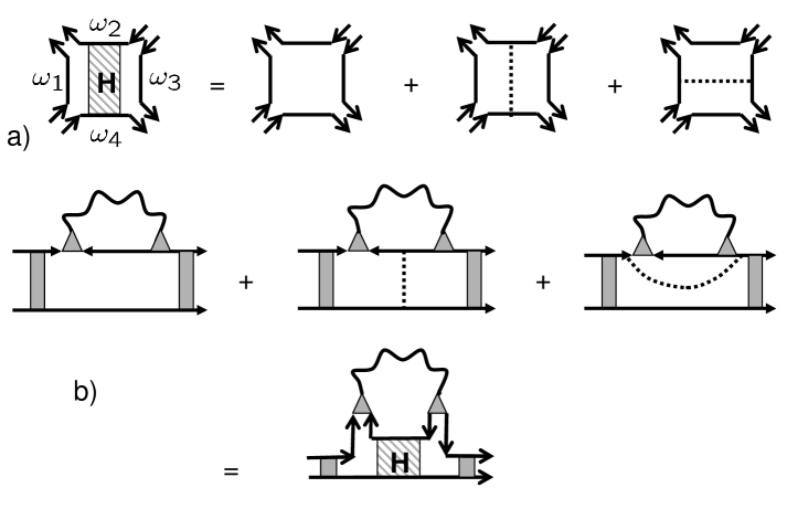
Figure 8: Diagrams $a)$ describe ”bosonic” Hikami box, Eq. (26). Using Hikami box the sum of three diagrams a), b) and c) in Fig. 3 can be conveniently represented as a single diagram shown in Fig. 6b. All notations are the same as in Fig. 3.

The sum of the diagrams d) and e) in Fig. 3 is given by

$$-\pi T^{2}\delta\sum\limits_{\varepsilon_{n}(\varepsilon_{n}-\Omega_{n})>0}\frac{K(\Omega_{n},\mathbf{q})}{\varepsilon_{n}^{2}(|2\varepsilon_{n}-\Omega_{n}|+\varepsilon_{\bf q}\delta)^{2}}\,\varepsilon_{\bf q}\delta.$$ (28)

The above expression for diagrams d) and e) in Fig. 3 in fact includes an additional contribution coming from the diagrams a), b) and c) in Fig. 3 that was not included in Eq. (27). This additional contribution appears due to the fact that the single electron Green function self-energy has a correction resulting from the renormalization of the Green function self-energy due to intergranular tunneling, see Eq. (10) and Fig. 4. This self energy correction is negligible in the diffusive limit ($\tau\to 0$), nevertheless it gives a finite contribution to the sum of the diagrams a) - c) because each of these diagrams diverge in the diffusive limit as $1/\tau$ while their sum remains finite due to cancellation of the leading orders in $1/\tau$. The additional finite term appears because the diagrams b) and c) have impurity lines that are determined by the bare mean free time $\tau_{0}$ while in all other places the mean free time appears through the Green function self energy that contains the renormalized $\tau.$ This additional contribution could have been written as an extra constant term $8\pi dg_{T}\delta$ in the Hikami box. We, however, find it is natural to ”redirect” this term to the diagrams d) and e) since these diagrams are also proportional to the tunnelling conductance $g_{T}.$

Finally, for the diagram f) in Fig. 3 we obtain

$$\pi T^{2}\delta\sum\limits_{\varepsilon_{n}(\varepsilon_{n}-\Omega_{n})<0}\frac{K(\Omega_{n},\mathbf{q})}{\varepsilon_{n}^{2}}\frac{1}{|\Omega_{n}|+\varepsilon_{\bf q}\delta}.$$ (29)

Adding all the contributions given by Eqs. (27)-(29) we obtain the correction to the superconducting transition temperature due to bosonic mechanism presented in Eq. (11).

Appendix B Evaluation of diagrams for the fermionic mechanism

In this appendix we evaluate diagrams for fermionic mechanism presented in Figs. 6 and 7 . We begin our analysis with the evaluation of the contribution $\langle X_{1}\rangle$ in the right hand side of Eq. (20) that can be written as a sum of two terms

$$\langle X_{1}\rangle=\langle X_{1}^{a}\rangle+\langle X_{1}^{b}\rangle,$$ (30a)

where $$\langle X_{1}^{a}\rangle \langle X_{1}^{b}\rangle$$ and represent the contributions of the diagrams a-f and g-j in Fig. 6 respectively. The sum of the diagrams a), b) and c) can be presented as a single diagram with the help of the Hikami box shown in Fig. 9a exactly as in the case of the bosonic diagrams considered in Appendix A. The corresponding Hikami box shown in Fig. 9a differs from the ”bosonic” Hikami box only by the arrow directions and is given by the same Eq. 26. The sum of the diagrams a), b) and c) in Fig. 6 thus results in the following expression

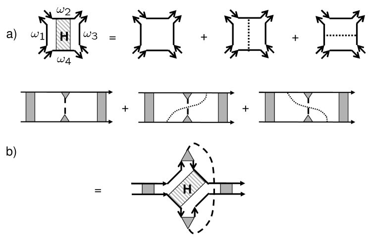
Figure 9: Diagrams a) describe ”fermionic” Hikami box. Using Hikami box the sum of three diagrams g), h) and i) in Fig. 6 can be conveniently represented as a single diagram b). All notations are the same as in Fig. 6 .

$$-2\pi T^{2}\sum\limits_{\varepsilon_{n}(\varepsilon_{n}-\Omega_{n})<0}\frac{\left(|\varepsilon_{n}|+|\Omega_{n}|/2\right)}{\varepsilon_{n}^{2}\,(|\Omega_{n}|+\varepsilon_{\bf q}\delta)^{2}}V(\Omega_{n},{\bf q}),$$ (30b)

where summation is going over the quasi-momentum, $\mathbf{q}$, fermionic, $\varepsilon_{n}$ and bosonic, $\Omega_{n}$ Matsubara frequencies. The propagator of the screened electron-electron interaction, $V(\Omega_{n},\mathbf{q})$ in Eq. (30b) was defined in Eq. (21c).

The sum of the diagrams d) and e) in Fig. 6 results in the following contribution

$$-\pi T^{2}\sum\limits_{\varepsilon_{n}(\varepsilon_{n}-\Omega_{n})<0}\frac{V(\Omega_{n},{\bf q})}{\varepsilon_{n}^{2}\,(|\Omega_{n}|+\varepsilon_{\bf q}\delta)^{2}}\,\varepsilon_{\bf q}\delta,$$ (30c)

while the diagram f) is given by

$$\pi T^{2}\sum\limits_{\varepsilon_{n}(\varepsilon_{n}-\Omega_{n})>0}\frac{V(\Omega_{n},{\bf q})}{\varepsilon_{n}^{2}\,(|2\varepsilon_{n}-\Omega_{n}|+\varepsilon_{\bf q}\delta)}.$$ (30d)

Summing up all contributions in Eqs. (30b)-(30d) we arrive to the following expression that represents the contribution of diagrams a)-f) in Fig. 6

$$\langle X_{1}^{a}\rangle=-\pi T^{2}\sum\limits_{{\bf q}}\left[\sum\limits_{\varepsilon_{n}(\varepsilon_{n}-\Omega_{n})<0}\left(\frac{2V(\Omega_{n},{\bf q})}{|\varepsilon_{n}|\,(|\Omega_{n}|+\varepsilon_{\bf q}\delta)^{2}}+\frac{V(\Omega_{n},{\bf q})}{\varepsilon_{n}^{2}(|\Omega_{n}|+\varepsilon_{\bf q}\delta)}\right)-\sum\limits_{\varepsilon_{n}(\varepsilon_{n}-\Omega_{n})>0}\frac{V(\Omega_{n},{\bf q})}{\varepsilon_{n}^{2}(|2\varepsilon_{n}-\Omega_{n}|+\varepsilon_{\bf q}\delta)}\right].\hskip 28.45274pt$$ (30e)

Now we turn to the evaluation of the diagrams g-j in Fig. 6 that are represented by the term $\langle X_{1}^{b}\rangle$ in Eq. (30a). Calculation of the sum of the diagrams g), h) and i) again can be reduced to the evaluation of a single diagram shown in Fig. 7b resulting in

$$-\pi T^{2}\sum\limits_{\varepsilon_{n}(\varepsilon_{n}-\Omega_{n})<0}\frac{|\Omega_{n}|\,\,V(\Omega_{n},{\bf q})}{(|\Omega_{n}|+\varepsilon_{\bf q}\delta)^{2}|\varepsilon_{n}||\varepsilon_{n}-\Omega_{n}|}.$$ (30f)

The diagram j) in Fig. 6 is given by the following expression

$$-\pi T^{2}\sum\limits_{\varepsilon_{n}(\varepsilon_{n}-\Omega_{n})<0}\frac{\varepsilon_{\bf q}\delta\,\,\,V(\Omega_{n},{\bf q})}{(|\Omega_{n}|+\varepsilon_{\bf q}\delta)^{2}|\varepsilon_{n}||\varepsilon_{n}-\Omega_{n}|},$$ (30g)

while the diagram k) results in

$$-\pi T^{2}\sum\limits_{\varepsilon_{n}(\varepsilon_{n}-\Omega_{n})>0}\frac{V(\Omega_{n},{\bf q})}{(|2\varepsilon_{n}-\Omega_{n}|+\varepsilon_{\bf q}\delta)|\varepsilon_{n}||\varepsilon_{n}-\Omega_{n}|}.$$ (30h)

Summing up the above contributions, Eqs. (30f) - (30h), we obtain the expression representing the sum of the diagrams g) - k) in Fig. 6

$$\langle X_{1}^{b}\rangle=-\pi T^{2}\sum\limits_{{\bf q}}\left[\sum\limits_{\varepsilon_{n}(\varepsilon_{n}-\Omega_{n})<0}\frac{V(\Omega_{n},{\bf q})}{|\varepsilon_{n}||\varepsilon_{n}-\Omega_{n}|(|\Omega_{n}|+\varepsilon_{\bf q}\delta)}+\sum\limits_{\varepsilon_{n}(\varepsilon_{n}-\Omega_{n})>0}\frac{V(\Omega_{n},{\bf q})}{|\varepsilon_{n}||\varepsilon_{n}-\Omega_{n}|(|2\varepsilon_{n}-\Omega_{n}|+\varepsilon_{\bf q}\delta)}\right].$$ (30i)

Now we turn to the evaluation of the vertex renormalization which is given by the term $\langle X_{2}\rangle$ in the right hand side of Eq. (20). The corresponding diagrams are shown in Fig. 7. Averaging over impurities results in the renormalization of the effective interaction vertex between the Coulomb and Cooper pair propagators. The renormalized vertex $\Gamma(\Omega_{n})$ is given by the sum of two diagrams shown in Fig. 7b that lead to the following expression

$$\Gamma(\Omega_{n})={T\over{\Omega_{n}+\varepsilon_{\bf q}\delta}}\sum_{0<\varepsilon_{n}<\Omega_{n}}{1\over\varepsilon_{n}}\,+\,T\sum_{\varepsilon_{n}>0}\left({1\over\varepsilon_{n}}-{1\over{\varepsilon_{n}+\Omega_{n}}}\right)\,{1\over{2\varepsilon_{n}+\Omega_{n}+\varepsilon_{\bf q}\delta}}.$$ (30j)

Using Eq. (30j) the resulting expression for the term $\langle X_{2}\rangle$ in Eq. (20) can be written as

$$\langle X_{2}\rangle=8\pi^{2}T\sum_{\mathbf{q},\Omega_{n}>0}V(\Omega_{n},\mathbf{q})\,K(\Omega_{n},\mathbf{q})\Gamma^{2}(\Omega_{n}),$$ (31)

where $K(\Omega_{n},\mathbf{q})$ is the propagator of superconducting fluctuations defined in Eq. (9). Expressing summations over the fermionic frequencies in Eqs. (30e, 30i) in terms of the di-gamma functions after some rearrangements of different terms in Eqs. (30e, 30i) we obtain Eq. (21a) for the suppression of superconducting transition temperature due to fermionic mechanism.

References

- (1) K. L. Ekinci and J. M. Valles, Jr., Phys. Rev. Lett. 82, 1518 (1999).
- (2) A. Gerber, A. Milner, G. Deutscher, M. Karpovsky, and A. Gladkikh, Phys. Rev. Lett. 78, 4277 (1997).
- (3) H. M. Jaeger, D. B. Haviland, A. M. Goldman, and B. G. Orr, Phys. Rev. B 34, 4920 (1986).
- (4) R. W. Simon, B. J. Dalrymple, D. Van Vechten, W. W. Fuller, and S. A. Wolf, Phys. Rev. B 36, 1962 (1987).
- (5) I. S. Beloborodov and K. B. Efetov, Phys. Rev. Lett. 82, 3332 (1999).
- (6) K. B. Efetov and A. Tschersich, Europhys. Lett. 59, 114, (2002); Phys. Rev. B 67, 174205 (2003).
- (7) P. W. Anderson, J. Phys. Chem. Solid 1, 26 (1959).
- (8) Yu. N. Ovchinnikov, Zh. Eksp. Teor. Fiz. 64, 719 (1973) [Sov. Phys. JETP 37, 366 (1973)].
- (9) S. Maekawa and H. Fukuyama, J. Phys. Soc. Jpn. 51, 1380 (1982); S. Maekawa, H. Ebisawa and H. Fukuyama, J. Phys. Soc. Jpn. 52, 1352 (1983).
- (10) A. M. Finkelstein, Pis’ma Zh. Eksp. Teor. Fiz. 45, 37 (1987) [Sov. Phys. JETP Lett. 45, 46 (1987)]; Phisica B 197, 636 (1994).
- (11) H. Ishida and R. Ikeda, J. Phys. Soc. Jpn. 67, 983 (1998); R. A. Smith, B. S. Handy and V. Ambegaokar, Phys. Rev. B 61, 6352 (2000).
- (12) A. I. Larkin, Ann. Phys. 8, 785 (1999).
- (13) K. B. Efetov, Zh. Eksp. Teor. Fiz. 78, 2017 (1980) [Sov. Phys. JETP 51, 1015 (1980)].
- (14) M. P. A. Fisher, Phys. Rev. Lett. 65, 923 (1990).
- (15) I. S. Beloborodov, K. B. Efetov, A. Altland and F. W. J. Hekking, Phys. Rev. B 63, 115109 (2001).
- (16) I. S. Beloborodov, K. B. Efetov, A. V. Lopatin and V. M. Vinokur, Phys. Rev. Lett. 91, 246801 (2003).
- (17) B. L. Altshuler and A. G. Aronov, in Electron-Electron Interaction in Disordered Systems, ed. by A. L. Efros and M. Pollak, North-Holland, Amsterdam (1985).
- (18) I. S. Beloborodov, A. V. Lopatin, and V. M. Vinokur, Phys. Rev. B, 70, 205120 (2004).
- (19) A. A. Abrikosov, L. P. Gorkov and I. E. Dzyaloshinskii, Methods of Quantum Field Theory in Statistical Physics (Prentice-Hall, Englewood Cliffs, NJ, 1963).
- (20) A. M. Finkelstein, Electron liquid in Disordered Conductors, edited by I. M. Khalatnikov, Soviet Scientific Reviews Vol. 14 (Harwood, London, 1990).
- (21) I. S. Beloborodov, A. V. Lopatin, and V. M. Vinokur, Phys. Rev. Lett. 92, 207002 (2004).
- (22) We thank Igor Aleiner for pointing this out.
- (23) S. Hikami, Phys. Rev. B 24, 2671 (1981).