Apex Exponents for Polymer–Probe Interactions

Abstract

We consider self-avoiding polymers attached to the tip of an impenetrable probe. The scaling exponents $\gamma_{1}$ and $\gamma_{2}$, characterizing the number of configurations for the attachment of the polymer by one end, or at its midpoint, vary continuously with the tip’s angle. These apex exponents are calculated analytically by $\epsilon$-expansion, and numerically by simulations in three dimensions. We find that when the polymer can move through the attachment point, it typically slides to one end; the apex exponents quantify the entropic barrier to threading the eye of the probe.

There has been remarkable progress in recent years in nanoprobing and single–molecule techniques. These developments have had a direct impact on biopolymer research producing a wealth of beautiful results on DNA dynamics Salman et al. (2001), molecular motors Davenport et al. (2000), and protein/RNA folding Fernandez and Li (2004); Liphardt et al. (2001). Today it is possible to measure statistical properties of a single macromolecule rather than deducing them from experiments with solutions of many polymers. This naturally leads to questions regarding the theoretical limitations of these techniques, such as the effects of microscopic probes on the measured properties of the polymer. Consider, for instance, a polymer attached to the apex of a cone–shaped probe (e.g. a micropipette or the tip of an atomic force microscope Clausen-Schaumann et al. (2000); Williams and Rouzina (2002)). What is the configurational entropy for this system? Suppose that this probe is a microscopic needle with a hole at the end. How hard is it to thread a polymer through the needle’s eye?

Quite generally, the number of configurations ${\mathfrak{N}}$ of a polymer of length $N$ or, equivalently, of an $N$–step self–avoiding walk (SAW), behaves as de Gennes (1979)

$${\mathfrak{N}}={\rm const}\times z^{N}N^{\gamma-1}.$$ (1)

The “effective coordination number” $z$, depends on microscopic details, while the exponent $\gamma$ is ‘universal.’ Actually, $\gamma$ does depend on geometric constraints which influence the polymer at all length scales. In particular, there are a number of results demonstrating the variations of $\gamma$ for polymers confined by wedges in two and three dimensions J. L. Cardy and S. Redner (1984); A. J. Guttmann and G. M. Torrie (1984); K. De’Bell and T. Lookman (1993); M. N. Barber et al. (1978): A SAW anchored at the origin and confined to a solid wedge (in 3D) or a planar wedge (in 2D) has an angle–dependent exponent $\gamma$ that diverges as the wedge angle vanishes. A limiting case which has been extensively studied, both analytically Kosmas (1985); Douglas and Kosmas (1989) and numerically M. N. Barber et al. (1978); K. De’Bell and T. Lookman (1993), is a SAW anchored to an impenetrable surface, for which $\gamma\equiv\gamma_{s}=0.70\pm 0.02$ M. N. Barber et al. (1978).

To model the polymer–probe system, we consider a SAW attached to the apex (tip) of an impenetrable obstacle (needle). To avoid introduction of an external length scale, we focus on obstacles of scale–invariant shape, such as a planar slice (sector) of angle $\alpha$ (Fig. 1a), or a conical needle of apex semi-angle $\beta$ (Fig. 1b). While both geometries are natural extensions of the 2D wedge, they are clearly different in three dimensions (and also distinct from the 3D wedge, which consists of two planes intersecting at a line). The former excludes the polymer from the volume of a cone, while the latter prevents it from crossing the surface of a slice. Nonetheless, the resulting phenomenology is rather similar. Indeed, one of the technical innovations of this paper is the demonstration that many such geometries can be treated in the same manner by an $\epsilon=4-d$ expansion focusing on the interaction with a 2D surface. The $\epsilon$–expansion, as well as numerical simulations in 3D, shows that the exponent $\gamma\equiv\gamma_{1}$ varies continuously with the apex opening angles in Fig. 1. Continuously varying exponents are rather uncommon in critical phenomena. In the present case they arise from the interaction of two self-similar entities, the polymer and the probe.

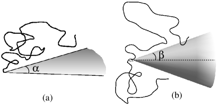
Figure 1: Configurations of a polymer near an obstacle: (a) attached to the apex of a planar sector of angle $\alpha$; (b) threaded through the eye of a cone with apex semi–angle $\beta$.

Another variant of this problem occurs when a polymer is attached to the apex at its midpoint. This case is described by Eq. (1) with exponent $\gamma\equiv\gamma_{2}$. More generally, let us denote by ${\mathfrak{N}}_{2}(N,N_{1})$, the number of accessible configurations for a polymer attached to the apex at an arbitrary monomer, dividing it in two segments of lengths $N_{1}$ and $N_{2}=N-N_{1}$. If we allow the two segments to exchange monomers with each other (which can be done by replacing a rigid attachment with a slip–ring as depicted in the Fig. 1b), then the equilibrium configurations will be distributed with a weight proportional to ${\mathfrak{N}}_{2}(N,N_{1})$. A natural interpolation formula as a function of $\alpha$ (or $\beta$), supported by the $\epsilon$-expansion at first order, is

$${\mathfrak{N}}_{2}(N,N_{1})\propto N^{c(\alpha)}[N_{1}(N-N_{1})]^{c_{1}(\alpha)}.$$ (2)

To get a feeling for this scaling relation, let us look at some limits: When the probe is absent, we recover Eq. (1) and $c(0)=\gamma_{0}-1$, where $\gamma_{0}\simeq 1.158$ describes the geometrically unconstrained SAW. If the obstacle is present but the two segments do not interact with each other, then $c=0$ and $c_{1}=\gamma_{1}-1$. By fitting to the limits of $N_{1}\to 0$ and $N_{1}\sim N_{2}$, we find $c_{1}=\gamma_{2}-\gamma_{1}$ and $c=2\gamma_{1}-\gamma_{2}-1$. Below, we estimate the exponents in Eq.(2) both analytically and numerically. For now, assuming Eq. (2) holds, we see that if $c_{1}<0$, the maximum number of configurations is realized when either $N_{1}$ or $N_{2}$ equals $N$. This brings us to one of our main findings: No matter how small the apex angle, we find $c_{1}<0$, i.e. the most likely states have $N_{1}\simeq N$ or $N_{2}\simeq N$, with an entropy barrier separating the two. Threading a needle is hard!

To treat the problem analytically, we start with the Edwards Edwards (1965) model of a self-avoiding polymer, and add an interaction with the obstacle. In this formulation, configurations of the polymer are described by ${\bf r}(\tau)\in\Re^{d}$, where $\tau$ measures the position along the chain, and are weighted according to the energy 

$${\cal H} = \frac{1}{2}\int_{0}^{N}\dot{\bf r}^{2}~{}d\tau+\frac{v_{0}}{2}\int_{0}^{N}d\tau\int_{0}^{N}d\tau^{\prime}\delta[{\bf r}(\tau)-{\bf r}(\tau^{\prime})]$$ (3)

$$+ g_{0}\int_{\mathcal{M}}d^{2}{\bf R}\int_{0}^{N}d\tau\delta[{\bf r}(\tau)-{\bf R}].$$

The self-avoiding interaction is replaced by a ‘soft’ repulsion of strength $v_{0}$. In the same spirit, the impenetrable obstacle is replaced with a soft repulsion of magnitude $g_{0}$. The key observation is that in 3D the polymer can only sense the exterior of an impenetrable obstacle, and will not care if its interior is hollow. In generalizing to $d$-dimensions, we keep the dimensions of the now softened exterior manifold (indicated by ${\bf R}\in{\mathcal{M}}$) as two. The advantage of this choice is that both $g_{0}$ and $v_{0}$ have the same bare dimensions, and in a perturbative scheme simultaneously become relevant in $d\leq 4$. We then analyze the model using a renormalization group (RG) scheme Kosmas (1985); Douglas and Kosmas (1989) which is a modification of the conformation space RG Oono et al. (1981); Freed (1987). The scaling exponents are calculated using dimensional regularization in $d=4-\epsilon$ dimensions to order $O(\epsilon)$.

Figure 2: Diagrams contributing to renormalization of $g$ to second order (a–c); to ${\mathcal{Z}}$ in first order (d,e) at the apex of a slice; and to ${\mathcal{Z}}_{2}$ in first order (f) at the eye of a conic needle.

It is customary to define non-dimensionalized (bare) coupling constants $\tilde{v}_{0}=v_{0}L^{\epsilon},~{}\tilde{g}_{0}=g_{0}L^{\epsilon}$ at a length scale $L$. We also define the renormalized coupling constants $v=Z^{-1}_{v}\tilde{v}_{0}$ and $g=Z^{-1}_{g}\tilde{g}_{0}$, where the renormalization constants $Z_{v}$, $Z_{g}$ are calculated perturbatively as series in $v$ and $g$. Diagrams contributing to the renormalization of $g$ are shown in Figs. 2a–c, and involve both interactions of the polymer with the obstacle and with itself. The leading singularity in $1/\epsilon$ comes from short distances and therefore the leading correction to $g$ does not depend on the overall shape of the obstacle. This is true as long as it is possible to draw a finite circle around points away from the apex (see Fig. 2b), and is also why the interaction with the obstacle becomes irrelevant in the degenerate limits of $\alpha=\beta=0$. The self–interaction is uninfluenced by the obstacle, and the renormalization constant $Z_{v}$ is the same as in the unattached polymer Freed (1987). To first order in $\epsilon$, the nontrivial fixed point of the RG flow is found to be $(v^{*},g^{*})=(\pi^{2}\epsilon/2,3\pi\epsilon/4)$. The fixed point thus depends only on the dimension of the constraining manifold, but not on its shape Freed (1983); Duplantier (1989). However, the number of accessible configurations does depend on the exact geometry as described below.

Consider first-order corrections to the partition function ${\mathcal{Z}}$ coming from the self–interaction (Fig. 2d) and the interaction with the slice (Fig. 2e). Combining them and adding relevant counterterms to eliminate poles in $\epsilon$, we obtain

$${\mathcal{Z}}=1+\frac{1}{4\pi^{2}}(v^{*}-\alpha g^{*})\ln\left(\frac{2\pi N}{L^{2}}\right)+O(\epsilon^{2}).$$ (4)

Comparing this with $N^{\gamma_{1}(\alpha)-1}=1+(\gamma_{1}(\alpha)-1)\ln N+\cdots$, and substituting the fixed point values $(v^{*},g^{*})$, we find

$$\gamma_{1}(\alpha)=1+\frac{\epsilon}{8}\left(1-\frac{3\alpha}{2\pi}\right)+O(\epsilon^{2}).$$ (5)

The above treatment is easily generalized to a polymer attached by its midpoint. For the number of configurations, we observe that the contribution from the interaction with the obstacle is doubled. Interaction between the two halves of the polymer, however, makes no separate correction and is already included. (Note that if we ignore the obstacle and consider self-interactions only, we get a “degenerate” star polymer with two branches that is equivalent to a linear polymer.) Thus, for the calculation of $\gamma_{2}$ at order of $\epsilon$, we can add the separate contributions from self-avoidance and avoidance of the obstacle; cross-terms can only occur at higher orders. This enables us to identify the scaling exponent

$$\gamma_{2}(\alpha)=1+\frac{\epsilon}{8}\left(1-\frac{3\alpha}{\pi}\right)+O(\epsilon^{2}).$$ (6)

Repeating this argument for the slip–ring geometry, we find

$${\mathfrak{N}}_{2}\propto N^{\epsilon/8}[N_{1}(N-N_{1})]^{-3\alpha\epsilon/(16\pi)},$$ (7)

which confirms the Ansatz in Eq. (2) to first order in $\epsilon$. Note that in 3D we must have $\gamma_{2}(2\pi)=2\gamma_{s}-1$. This equality does not hold in the $\epsilon$–expansion. The reason is that in 3D, a complete plane prevents two polymers on its opposite sides from interacting with each other, whereas in 4D it does not.

It is straightforward to extend the above formalism to obstacles of different shapes, such as the conical manifold with apex angle $\beta$ (Fig. 1b). In counting the number of configurations we obtain a result similar to Eq. (4), with $\alpha$ replaced by $2\pi\sin\beta$. Since the fixed point location is the same as before, this substitution in Eqs. (5-6) gives

$$\gamma_{1}^{\rm cone}(\beta) = 1+\frac{\epsilon}{8}(1-3\sin\beta)+O(\epsilon^{2}),$$ (8)

$${\mathfrak{N}}_{2}^{\rm cone}(\beta) \propto N^{\epsilon/8}[N_{1}(N-N_{1})]^{-(3/8)\epsilon\sin\beta}.$$ (9)

The difference between the two geometries is thus merely quantitative. As another point of caution, we note that within our formalism, the polymer is free to occupy either side of the hollow cone– the partition sum is dominated by the arrangement with the largest number of configurations. Thus the result for $\gamma_{1}(\beta)$ is valid only for $\beta\leq\pi/2$, with a possibly more severe restriction for $\gamma_{2}$.

The earlier discussion of ‘threading a needle’ illustrates the essence of the method of “entropic competition” Zandi et al. (2003); Marcone et al. (2004) which we employ to numerically estimate the exponents $\gamma_{i}(\alpha)$ in 3D. The underlying idea is to sample the ensemble of different configurations of two polymer segments which can exchange monomers and thus “compete entropically” (e.g. in a slip–ring geometry). To calculate $\gamma_{1}(\alpha)$, we prevent the two segments from interacting with each other. The number of configurations for given $N$ and $N_{2}=N-N_{1}$ is then

$${\mathfrak{N}}_{1}\propto[N_{1}(N-N_{1})]^{\gamma_{1}(\alpha)-1},$$ (10)

so that the resulting histogram for $N_{1}$ allows us to calculate the exponent $\gamma_{1}(\alpha)$. In our simulations we consider sectors with angles $\alpha=k\pi/8$, where $k=0,1,2,\dots,16$. We work on a cubic lattice, with the excluded sector in the $x-y$ plane. Possible Monte Carlo (MC) moves include attempts to remove one monomer from the free end of a randomly chosen polymer segment and adding it to the free end of the other segment; both segments also undergo random configuration changes via pivoting N. Madras and A. D. Sokal (1988). Figure 3 illustrates the dramatic effect of the angle $\alpha$ on $p(N_{1})$, the probability distribution function (PDF) for the segment length $N_{1}$. For small $\alpha$, the distribution is peaked at the center while for $\alpha$ bigger than a critical value $\alpha_{c}$, the maximum of the PDF moves to the sides. The numerical data from entropic competition suggest $\alpha_{c}\approx 5\pi/8$, which is not too far from the first order $\epsilon$–expansion result of $\alpha_{c}=2\pi/3$ in Eq. (5).

For the purpose of calculating $\gamma_{2}(\alpha)$, it is necessary to include interactions between the segments. Figure 4 depicts variations of the exponents $\gamma_{1,2}(\alpha)$ obtained by fitting histograms from entropic competition, such as in Fig. 3, to power-laws as in Eqs. (10) and (2).

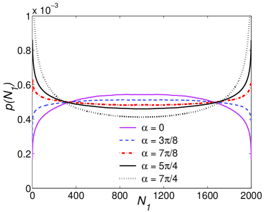
Figure 3: The probability distributions $p(N_{1})$ for two non-interacting segments of lengths $N_{1}$ and $N-N_{1}$ attached to the apex of a planar slice for diffrent values of angle $\alpha$. The curves are the result of $10^{9}$ MC steps for $N=2000$.

It is instructive to compare the results of entropic competition with those of a more established procedure, such as dimerization Suzuki (1968); Alexandrowicz (1969). The latter is a quite efficient method N. Madras and A. D. Sokal (1988), in which an $N$-step SAW is created by generating two $(N/2)$-step SAWs and attempting to concatenate them. We generated SAWs for $N=16,~{}32,\cdots~{},2048$, and by attempting to attach them to the end point of an appropriate sector, measured a success probability $p_{N}$. Let us indicate the number of SAWs not attached to the sector by $A_{0}z^{N}N^{\gamma_{0}-1}$, and those attached to the sector either (1) by their ends, or (2) by their mid-point as $A_{i}z^{N}N^{\gamma_{i}(\alpha)-1}$ ($i=1,2$ corresponds to the notation introduced earlier). Then, the ratio between the number of configurations, $p_{N}\equiv(A_{i}/A_{0})N^{\gamma_{i}(\alpha)-\gamma_{0}}$, represents the probability to attach an $N$–step polymer to a sector with angle $\alpha$. Fitting a power law to this ratio thus provides a means of estimating the exponent difference $\Delta\gamma_{i}\equiv\gamma_{0}-\gamma_{i}$.

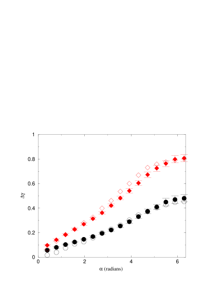
Figure 4: Extrapolated values of the exponents $\Delta\gamma_{1}=\gamma_{0}-\gamma_{1}$ (circles) and $\Delta\gamma_{2}=\gamma_{0}-\gamma_{2}$ (diamonds) as a function of sector angle $\alpha$ from ‘entropic competition’ (open symbols), and dimerization (full symbols). Error bars represent statistical uncertainties of individual estimates of the exponents, as well as the uncertainty in the extrapolation $N\to\infty$.

Using the dimerization method we generated $M=10^{6}$ SAWs; for each we checked whether there is an intersection with sectors at all tested values of $\alpha$ . The error in the measurement of $p_{N}$ is $\sqrt{p_{N}(1-p_{N})/M}$. Since $p_{N}$ decreases with increasing angle of the sector, the relative error in $p_{N}$, and an error in the estimates of $\Delta\gamma_{i}$, increases with increasing $\alpha$. Nevertheless, we were able to obtain reasonable estimates of the exponent for all values of $\alpha$, as shown in Fig. 4 (full symbols).

The two numerical approaches are in very good agreement; error bars for ‘entropic competition’ results being even smaller. For $\alpha=0$, our results deviate from zero beyond the statistical error range. We believe this deviation to be a finite size effect, due to discreteness of the lattice. As a check, we estimated $\Delta\gamma_{1,2}$ when the obstacle consists of the positive $x$-axis. While asymptotically such a situation corresponds to $\alpha=0$, and should lead to $\Delta\gamma_{i}=0$, we obtained $\Delta\gamma_{1}=0.02$ and $\Delta\gamma_{2}=0.05$. For $\alpha=2\pi$, we expect to have $\Delta\gamma_{1}=\gamma_{0}-\gamma_{s}\approx 0.46$, and $\Delta\gamma_{2}=\gamma_{0}-2\gamma_{s}+1\approx 0.76$; our results are quite close to these estimates.

In summary, we consider configurations of a polymer attached to the apex of a self-similar probe (at least on the scale of the polymer size). The geometric constraints imposed by the impenetrable probe lead to exponents continuously with the apex angle. Two such exponents are associated with attachment of the polymer by one end or by a mid-point. Together, they determine if a mobile attachment point is likely to be in the middle or slide to one side. These apex exponents are obtained analytically by an $\epsilon=4-d$ expansion, and through independent numerical schemes in $d=3$. The $\epsilon$-expansion takes advantage of the marginality of interactions of a polymer with a two dimensional manifold in four dimensions, and can be applied to a variety of shapes. The numerical method of ‘entropic competition’ is shown to be a powerful tool in this context, comparable to or better than the more standard dimerization approach. The numerical and analytical results are in agreement, and indicate the presence of an entropic barrier that favors attachment of the polymer to the apex at its end. It would be interesting to see if these predictions can be probed by single molecule experiments.

This work was supported by Israel Science Foundation grant No. 38/02, and by the National Science Foundation grant DMR-01-18213.

References

- Salman et al. (2001) H. Salman, D. Zbaida, Y. Rabin, D. Chatenay, and M. Elbaum, Proc. Nat. Acad. Sci. USA 98, 7247 (2001).
- Davenport et al. (2000) R. J. Davenport, G. J. Wuite, R. Landick, and C. Bustamante, Science 287, 2497 (2000).
- Fernandez and Li (2004) J. M. Fernandez and H. Li, Science 303, 1674 (2004).
- Liphardt et al. (2001) J. Liphardt, B. Onoa, S. B. Smith, I. Tinoco, Jr., and C. Bustamante, Science 292, 733 (2001).
- Clausen-Schaumann et al. (2000) H. Clausen-Schaumann, M. Seitz, R. Krautbauer, and H. Gaub, Curr. Opin. Chem. Biol. 4, 524 (2000).
- Williams and Rouzina (2002) M. Williams and I. Rouzina, Curr. Opin. Struct. Biol. 12, 330 (2002).
- de Gennes (1979) P. G. de Gennes, Scaling Concepts in Polymer Physics (Cornell University Press, Ithaca, New York, 1979).
- J. L. Cardy and S. Redner (1984) J. L. Cardy and S. Redner, J. Phys. A 17, L933 (1984).
- A. J. Guttmann and G. M. Torrie (1984) A. J. Guttmann and G. M. Torrie, J. Phys. A 17, 3539 (1984).
- K. De’Bell and T. Lookman (1993) K. De’Bell and T. Lookman, Rev. Mod. Phys. 65, 87 (1993).
- M. N. Barber et al. (1978) M. N. Barber, A. J. Guttmann, K. M. Middlemiss, G. M. Torrie, and S. G. Whittington, J. Phys. A 11, 1833 (1978).
- Kosmas (1985) M. K. Kosmas, J. Phys. A 18, 539 (1985).
- Douglas and Kosmas (1989) J. Douglas and M. Kosmas, Macromolecules 22, 2412 (1989).
- Edwards (1965) S. F. Edwards, Proc. Phys. Soc. London 85, 613 (1965).
- Oono et al. (1981) Y. Oono, T. Ohta, and K. F. Freed, J. Chem. Phys. 74, 6458 (1981).
- Freed (1987) K. F. Freed, Renormalization group theory of macromolecules (J. Wiley, New York, 1987).
- Freed (1983) K. F. Freed, J. Chem. Phys. 79, 3121 (1983).
- Duplantier (1989) B. Duplantier, Phys. Rev. Lett. 62, 2337 (1989).
- Zandi et al. (2003) R. Zandi, Y. Kantor, and M. Kardar, ARI 53, 6 (2003), cond-mat/0306587.
- Marcone et al. (2004) B. Marcone, E. Orlandini, A. Stella, and F. Zonta (2004), cond-mat/0405253.
- N. Madras and A. D. Sokal (1988) N. Madras and A. D. Sokal, J. Stat. Phys 50, 109 (1988).
- Suzuki (1968) K. Suzuki, Bull. Chem. Soc. Japan 41, 538 (1968).
- Alexandrowicz (1969) Z. Alexandrowicz, J. Comp. Phys. 51, 561 (1969).