Spin-orbit coupling and anisotropy of spin splitting in quantum dots

Abstract

In lateral quantum dots, the combined effect of both Dresselhaus and Bychkov-Rashba spin orbit coupling is equivalent to an effective magnetic field $\pm B_{so}$ which has the opposite sign for $s_{z}=\pm 1/2$ spin electrons. When the external magnetic field is perpendicular to the planar structure, the field $B_{so}$ generates an additional splitting for electron states as compared to the spin splitting in the in-plane field orientation. The anisotropy of spin splitting has been measured and then analyzed in terms of spin-orbit coupling in several AlGaAs/GaAs quantum dots by means of resonant tunneling spectroscopy. From the measured values and sign of the anisotropy we are able to determine the dominating spin-orbit coupling mechanism.

A better understanding of the spin-orbit (SO) effects is crucial for the implementation of the coherent manipulation of the electron spin SpinManip ; SpinQubits in quantum dots and wires. SO coupling in III-V semiconductor structures is usually composed of two interplaying contributions of different symmetries,

$$\mathcal{H}_{\mathrm{so}}=\varrho_{\mathrm{D}}(p_{x}s_{x}-p_{y}s_{y})+\varrho_{\mathrm{BR}}(p_{y}s_{x}-p_{x}s_{y})\mathbf{.}$$ (1)

The first term is reminiscent of the Dresselhaus SO coupling in zink-blend bulk semiconductors Dress ; Dresselhaus (it reflects the inversion-asymmetry of GaAs). The second term in Eq. (1) is the interface-induced coupling of Bychkov-Rashba type Rashba . It is difficult to separate the effects of the two SO coupling mechanisms in quantum transport measurements and spin relaxation Rossler ; WeakLoc ; AF ; BF ; Zumbuehl ; Shayegan , (except for optical experiments Jusserand ; Ganichev ), and even to determine which one is dominant. At the same time coherent spin manipulation as well as the spin-Hall effect SpinManip ; SpinManip2 ; Loss depend on the balance between the two mechanisms.

In this Letter, we show that the relative strength of the Dresselhaus and Bychkov-Rashba SO coupling mechanisms in a particular device can be determined from the anisotropy of the Zeeman spin splitting. Experimentally, we exploit the method of single-electron resonant tunneling spectroscopy Haug to observe the difference $\Delta_{\bot}-\Delta_{\|}$ in spin splitting of single-electron resonances in a double-barrier structure subjected to a magnetic field perpendicular ($\Delta_{\bot}$) and parallel ($\Delta_{\|}$) to the plane of the quantum well. We analyze this anisotropy within the framework of the theory of SO coupling in lateral quantum dots AF ; BF . It is shown below that the two mechanisms cause anisotropy of opposite signs, and that

$$\Delta_{\bot}-\Delta_{\|}\propto\left(-g/|g|\right)\left(\varrho_{\mathrm{BR}}^{2}-\varrho_{\mathrm{D}}^{2}\right),$$ (2)

where $g$ is the quantum well electron Lande g-factor in the in-plane magnetic field.

The experiment was performed with two highly asymmetric double barrier resonant tunneling devices grown by molecular beam epitaxy on n+-type GaAs substrate. In both samples the undoped 10 nm wide GaAs quantum well is sandwiched between 5 and 8 nm thick Al_0.3Ga_0.7As tunneling barriers separated from the highly doped GaAs contacts (Si-doped with $n_{S}=4\times 10^{17}$ cm^-3) by 7 nm thick undoped GaAs spacer layers. The samples were fabricated as pillars of $2$ $\mu$m (sample A) and $40$ $\mu$m diameter (sample B). DC measurements of the I-V characteristics were performed in two devices in a dilution refrigerator at $20$ mK base temperature for two different orientations of magnetic field, see Fig. 1 (a).

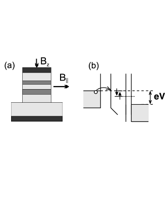
Figure 1: Schematic picture (a) and energy diagram (b) of the studied device under finite bias and finite magnetic field.

The studied GaAs quantum well embedded between two AlGaAs barriers can be viewed as a two-dimensional system with the edges and residual impurities confining the lateral electron motion and thus forming dots. Tunneling through the lowest state of the dot, at the energy $E_{0}$ and with lateral extent $\lambda$, produces the lowest resonance peak in the differential conductance, whereas its excited states are responsible for additional peaks in dI/dV, which all move in a magnetic field $B_{z}$ perpendicular to the quantum well, as shown in Figs. 2 and 3. The magnetic field dependence of energy levels can be illustrated using the model of parabolic confinement, $V(\mathbf{r})=\tfrac{1}{2}m\omega^{2}\mathbf{r}^{2}$, with the extension of the wavefunction $\lambda\sim\sqrt{\hbar/\omega m}$, where the spectrum of quantum dot states $|n_{+}n_{-}\rangle$, $n_{\pm}=0,1,2,\dots$ is described by

$$E_{n_{+}n_{-}} = E_{0}+\hbar\sqrt{\omega^{2}+\left(\omega_{c}/2\right)^{2}}-\hbar\omega+\sum_{\pm}n_{\pm}\hbar\omega_{\pm}$$

$$\omega_{\pm} = \sqrt{\omega^{2}+\left(\omega_{c}/2\right)^{2}}\pm\tfrac{1}{2}\omega_{c},\mbox{ }\omega_{c}=eB/m.$$ (3)

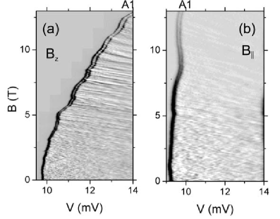
Figure 2: Differential conductance as a grey-scale plot for sample A ($\hbar\omega=31.2$ meV) as a function of bias voltage and magnetic field for (a) $B_{z}$ being perpendicular to the quantum well plane and (b) $B_{\parallel}$, T=20 mK.

For a strongly bound state or at low fields, such that $\omega>\omega_{c}$ (also $\lambda<\lambda_{B}$, where $\lambda_{B}=\sqrt{\hbar/eB_{z}}$), the first tunneling resonance experiences a diamagnetic shift $E_{00}\approx E_{0}+\hbar\omega_{c}^{2}/8\omega$, which is quadratic in $B_{z}$. For an electron localized near a smooth potential minimum, such that $\omega\ll\omega_{c}$ at high fields, $\omega_{+}\approx\omega_{c}$ and $\omega_{-}\approx\omega^{2}/\omega_{c}\ll\omega_{c}$, the diamagnetic shift of several low-energy states in a dot follows approximately the energy of the lowest 2D Landau level, $E_{0n_{-}}\approx\left[E_{0}-\hbar\omega+(n_{-}+1)\hbar\omega^{2}/\omega_{c}\right]+1/2\hbar\omega_{c}(B_{z})$.  In the structures studied, both weakly and strongly bound states have been seen.

Fig. 2 (a) shows the differential conductance peak A1 found in sample A and attributed to a strongly bound state ($\hbar\omega=31.2$ meV), presumably, formed by a growth-induced local potential minimum. Several differential conductance peaks B1-B4 and BX were observed in sample B, with a smaller energy separation. The magnetic field dependence of their positions shown in Fig. 3(a) complies with the magneto-spectrum in a parabolic potential with $\hbar\omega=13.8$ meV footnote2 . The data shown in Fig. 2 (b) and 3(b), which have been taken on the same structures subjected to an in-plane magnetic field of comparable strength, do not display a diamagnetic shift and confirm the 2D nature of the dots.

In both magnetic field directions, all peaks in dI/dV resolve into two at high enough field values, manifesting the spin splitting of each dot state. Spin splittings extracted from the set of data shown in Figs. 2 and 3 are gathered in Fig. 4: (a) shows the data for sample A, whereas (b) shows the field dependence of splittings in sample B.

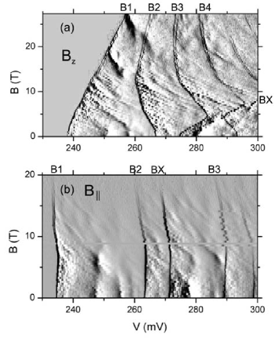
Figure 3: Differential conductance as a grey-scale plot for sample B ($\hbar\omega=13.8$ meV) as a function of bias voltage and magnetic field for (a) $B_{z}$ being perpendicular to the quantum well plane and (b) $B_{\parallel}$, T=20 mK.

The data shown in Fig. 4 display a distinct anisotropy of the peak splitting, with the splitting caused by the out-of-plane field (open symbols) being systematically larger than what is created by the in-plane field (closed symbols).

The observed values of spin splitting anisotropy are much larger and have the opposite sign to what might be expected from the kinetic energy dependence, $g=-0.44+E\cdot dg/dE$ of the electron g-factor across the conduction band in GaAs. Using $dg/dE\sim+2$ $\mathrm{eV}^{-1}$Snelling , we estimate that the diamagnetic shift (which increases the electron kinetic energy in a perpendicular magnetic field) would further reduce the value of $g$ at higher fields by $(\hbar\omega_{c}/2)\cdot(dg/dE)$. The latter is less than the observed anisotropy in the peak B1. One may also notice that the anisotropy of spin splitting of the excited dot states B2-B4 shown in the inset to Fig. 4 is the same as of B1, despite a larger kinetic energy of an electron in them.

Below we show that the observed spin splitting anisotropy can be attributed to the effect of SO coupling in the lateral electron motion in a narrow quantum well, and that its values observed in various dot states in both samples A and B can be traced down to the same SO coupling characteristics, namely, the effective SO-induced magnetic field $B_{\mathrm{so}}=(\hbar m^{2})/(2e)(\varrho_{\mathrm{BR}}^{2}-\varrho_{\mathrm{D}}^{2})$.

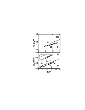
Figure 4: (a) Spin splitting of the state A1 of sample A for both B-field configurations. (b) Spin splitting of the state B1 of sample B for both B-field configurations. Solid and dotted lines are discussed in the text. Inset shows the spin splitting of the states B2-B4 of sample B for both B-field configurations.

For a quantum well lying in the (001) crystallographic plane of GaAs it is convenient to choose coordinates along crystallographic directions $\mathbf{\hat{e}}_{1}=[110]$ and $\mathbf{\hat{e}}_{2}=[\bar{1}10]$, and to study the effective 2D Hamiltonian in the form

$$\mathcal{H}\! = \!\frac{\left(-i\hbar\nabla\mathbf{-A}-\mathbf{a}\right)^{2}}{2m}+\dfrac{g}{|g|}\dfrac{\epsilon_{\mathrm{Z}}}{2}\mathbf{l\sigma}+V(\mathbf{r}),\;$$ (4)

$$\mathbf{a} \mathbf{=} \frac{\hbar\sigma_{2}\mathbf{\hat{e}}_{1}}{2\lambda_{1}}-\frac{\hbar\sigma_{1}\mathbf{\hat{e}}_{2}}{2\lambda_{2}}$$ (5)

where $\mathbf{A}=\tfrac{e}{2}B_{z}[\mathbf{r\times\hat{e}}_{z}]$, $\mathbf{l=B}/B$, $\mathbf{\sigma}=(\sigma_{1},\sigma_{2},\sigma_{3})$ is the vector of Pauli matrices, and $\epsilon_{\mathrm{Z}}=|g\mu_{\mathrm{B}}B|$ is the Zeeman energy (in a 10nm wide GaAs/AlGaAs quantum well, $g<0$ according to Snelling et al Snelling , and in the above expressions we have already taken into account the negative sign of the electron charge, so that $e>0$). The parameters $\varrho_{\mathrm{D}}$ and $\varrho_{\mathrm{BR}}$ of the SO coupling defined in Eq. (1) for a conventional choice of axes, $\mathbf{\hat{x}}=[100]$ and $\mathbf{\hat{y}}=[010]$ appear in the uniform non-Abelian vector potential $\mathbf{a}$ in Eq. (4) via the inverse of the SO coupling length $\lambda_{1(2)}$ as $\lambda_{1}^{-1}=\left(\varrho_{\mathrm{D}}-\varrho_{\mathrm{BR}}\right)m$ and $\lambda_{2}^{-1}=-\left(\varrho_{\mathrm{BR}}+\varrho_{\mathrm{D}}\right)m$, where $2\pi\lambda_{1(2)}$ characterizes the distance at which spin precession of a polarised electron moving along crystallographic direction $\mathbf{\hat{e}}_{1(2)}$ undergoes one complete revolution.

To analyze the case of a weak SO coupling for electrons bound in a small-size quantum dot, $\lambda_{1,2}\gg\lambda$, we follow Refs. AF ; BF and perform a non-uniform unitary transformation to the electron wave function, $\psi(\mathbf{r})=U(\mathbf{r})\tilde{\psi}(\mathbf{r})$ and the Hamiltonian in Eq. (4),

$$U=\exp\left\{\tfrac{i}{2}\left[\lambda_{1}^{-1}x_{1}\sigma_{2}-\lambda_{2}^{-1}x_{2}\sigma_{1}\right]\right\},\;\mathcal{\tilde{H}}=U^{\dagger}\mathcal{H}U.$$

This transformation rotates locally the spin space by the angle $R=\sqrt{\left(x_{1}/\lambda_{1}\right)^{2}+\left(x_{2}/\lambda_{2}\right)^{2}}$ around the unit vector $\mathbf{\hat{n}}\mathbf{=}\left(\lambda_{1}^{-1}x_{1}\mathbf{\hat{e}}_{2}-\lambda_{2}^{-1}x_{2}\mathbf{\hat{e}}_{1}\right)/R$. As a result the coordinate frame for the electron spin set in the center of the dot, $x_{1,2}=0$ gets adjusted to the local orientation determined by the SO-induced spin precession upon its displacement along the radius vector $\mathbf{r}$. The enrgy spectrum can be found from the transformed Hamiltonian

$$\mathcal{\tilde{H}}=\!\frac{1}{2m}\left(-i\hbar\nabla\mathbf{-A}-\mathbf{\tilde{a}}\right)^{2}+\tfrac{1}{2}\epsilon_{\mathrm{Z}}\mathbf{\tilde{l}\sigma}+V(\mathbf{r}),$$

where $\mathbf{\tilde{a}}=U^{\dagger}\mathbf{a}U+i\hbar U^{\dagger}\nabla U$ and $\mathbf{\tilde{l}}(\mathbf{r})=(\mathbf{l\cdot\hat{n})\hat{n}+\hat{n}\mathbf{\times}\left[\mathbf{l\times\hat{n}}\right]}\cos R-\mathbf{\left[\mathbf{l\times\hat{n}}\right]}\sin R$. The transformation $U(\mathbf{r})$ aims to gauge out Gefen ; MathurStone ; AF ; BF spin-orbit coupling, which appears in Eq. (4) in the form of uniform spin-dependent vector potential in Eq. (5). The latter goal cannot be achieved in full, since Pauli matrices do not commute with each other. However, for a weak SO coupling [$\lambda_{1,2}\gg\lambda$] and small rotation angles $R\ll 1$, the residual $\mathbf{\tilde{a}}$ , BF

$$\mathbf{\tilde{a}}=-\frac{[\mathbf{r}\times\mathbf{\hat{e}}_{3}]}{4\lambda_{1}\lambda_{2}}\hbar\sigma_{3}+\hbar\lambda_{1,2}^{-1}\mathcal{O}[R^{2}],$$ (6)

is dominated Footnote1 ; footnote3 by the ’vector potential’ of an effective magnetic field which has the opposite sign for spin ”up” and ”down” electrons in the quantum dot, AF ; BF

$$B_{\mathrm{eff}}=B_{z}-\sigma_{3}B_{\mathrm{so}}.$$ (7)

It is this difference in the effective magnetic field seen by an electron in the adjusted spin frame that causes the spin splitting anisotropy. For the in-plane magnetic field orientation ($B_{z}=0$), the effective field $B_{\mathrm{eff}}=\pm B_{\mathrm{so}}$ produces the same negligibly small ’diamagnetic’ shift $\sim B_{\mathrm{so}}^{2}$ in the orbital motion energy of both spin components. Accordingly it does not alter the value of the quantum well Zeeman splitting, $\Delta_{\|}=\epsilon_{\mathrm{Z}}$.

For the perpendicular magnetic field orientation ($\mathbf{B}=B\mathbf{\hat{e}}_{z}$), the difference in $B_{\mathrm{eff}}=B_{z}\pm B_{\mathrm{so}}$ generates the difference in the effective diamagnetic shift for two spin states and, therefore, an additional energy splitting. It results in the anisotropy of spin splitting in the lowest quantum dot state

$$\Delta_{\bot}-\Delta_{\|}=\dfrac{-g}{|g|}\dfrac{dE_{00}}{dB_{z}}2B_{\mathrm{so}}=\dfrac{-g}{|g|}\dfrac{\dfrac{\omega_{c}}{2}\dfrac{e\hbar}{m}B_{\mathrm{so}}}{\sqrt{\omega^{2}+\left(\tfrac{1}{2}\omega_{c}\right)^{2}}}.$$ (8)

Eq. (8) is valid in both low and high magnetic field regimes. Its low-field asymptotic

$$\Delta_{\bot}-\Delta_{\|}\approx\left(\dfrac{-g}{|g|}\right)B\hbar e^{2}B_{\mathrm{so}}/(2\omega m^{2})$$ (9)

for $\omega_{c}<\omega$ also describes the situation of a strongly bound electron, such as the resonance level A1. In the latter case, it is linear in the external field and looks like the anisotropy of the Lande factor. The high-field asymptotic of the result in Eq. (8),

$$\Delta_{\bot}-\Delta_{\|}\approx\left(\dfrac{-g}{|g|}\right)\dfrac{e\hbar}{m}B_{\mathrm{so}}\;\;\mathrm{for}\;\omega_{c}\gg\omega,$$ (10)

simultaneously describes the anisotropy of the spin splitting of the few lowest quantum dot states $E_{0n_{-}}$. For all of them, the anisotropy energy transforms into an offset with the sign dependent on the sign of $B_{\mathrm{so}}\propto(\varrho_{\mathrm{BR}}^{2}-\varrho_{\mathrm{D}}^{2})$ in Eq. (7) and on the sign of the electron g-factor.
Finally, we apply Eqs. (8-10) to analyze the peak splitting data shown in Fig. 4. Since in a 10nm-wide GaAs quantum well the bare value of g-factor is negative Snelling , larger values of spin splitting in a perpendicular field mean that $B_{\mathrm{so}}\propto(\varrho_{\mathrm{BR}}^{2}-\varrho_{\mathrm{D}}^{2})>0$, pointing at the dominance of the Bychkov-Rashba term in the SO coupling, presumably, due to the electron penetrating into the AlGaAs barrier which is enhanced in a narrow quantum well.

The fit to the experimentally observed anisotropy produces the values of the parameter $(e\hbar/m)\cdot B_{\mathrm{so}}$ which are shown in Table 1 and can be used to determine the effective field $B_{\mathrm{so}}$ in each sample.  For sample B, the two extracted values of $B_{\mathrm{so}}=25\pm 6$ mT for B1 and $25\pm 8$ mT for B2-B4 were obtained using Eq. (10) and agree to each other. The strongly confined state observed in sample A [peak A1, Fig. 4(a)] was analyzed using the result in Eq. (9), and as a result we extracted $B_{\mathrm{so}}=19\pm 1$ mT.

sample	A	B
peak	A1	B1          B2-B4
$\dfrac{e\hbar}{m}B_{\mathrm{so}}$	$32\pm 2$ $\mathrm{\mu eV}$	$43\pm 10$ $\mathrm{\mu eV}$ $44\pm 16$ $\mathrm{\mu eV}$
$B_{\mathrm{so}}$	$19$ mT	$25$ mT

Table 1: Experimental parameters of the spin-orbit characteristics for sample A and B, as discussed in the text.

The sign of SO coupling characteristics in $B_{\mathrm{so}}\propto(\varrho_{\mathrm{BR}}^{2}-\varrho_{\mathrm{D}}^{2})$ suggests that in a narrow quantum well Bychkov-Rashba coupling is dominant - in contrast to wide quantum wells investigated in Raman scatteringJusserand . The extracted SO coupling is also stronger than that estimated from the bulk Dresselhaus term, $2\gamma\hbar^{-4}\sum_{ijk}\epsilon^{ijk}p_{i}^{2}p_{j}s_{j}$, (where $\epsilon^{ijk}$ is anti-symmetric tensor) using $\gamma=\left(26\pm 5\right)$ $\mathrm{eV\mathring{A}}^{3}$ collected from references Jusserand ; WeakLoc . For the quantum well width $w=10$nm, the Dresselhaus mechanism alone would generate $B_{\mathrm{so}}$ which reduces the Zeeman splitting and is of much smaller absolute value, $\hbar^{2}m/2\varrho_{\mathrm{D}}^{2}\approx 2\pi^{4}m(\gamma/w^{2})^{2}\approx 12$ $\mathrm{\mu eV}$. Using this estimate, we can deduce the strength of the Bychkov-Rashba coupling in quantum wells in the samples B(A) as, at least, $(\hbar^{2}m/2)\cdot\varrho_{\mathrm{BR}}^{2}\sim 54(44)$ $\mathrm{\mu eV}$.

We acknowledge sample growth by A. Förster, H. Lüth, V. Avrutin and A. Waag. This work was partially supported by BMBF (RH), DFG (RH), by EPSRC (VF), DARPA under the QuIST Program (BA), and by ARDA/ARO Quantum Computing Program (BA).

References

- (1) J. M. Elzerman et al, Phys. Rev. B 67, 161308 (2003); R. Hanson et al, Phys. Rev. Lett. 91, 196802 (2003)
- (2) D. Loss and D. P. DiVincenzo, Phys. Rev. A 57, 120-126 (1998), G. Burkard and D. Loss, Phys. Rev. Lett. 88, 047903 (2002); D. Stepanenko et al, Phys. Rev. B 68, 115306 (2003)
- (3) G. Dresselhaus, Phys. Rev. 100, 580 (1955).
- (4) F. Malcher, G. Lommer, U. Rössler, Superlatt. Microstruct. 2, 267 (1986).
- (5) Yu. Bychkov and E. Rashba, JETP Lett. 39, 78 (1984); L. Wissinger et al, Phys. Rev. B 58, 15375-15377 (1998).
- (6) F.Malcher, G.Lommer, U.Rössler, Phys. Rev. Lett. 60, 728 (1988).
- (7) J. B. Miller et al, Phys. Rev. Lett. 90, 076807 (2003); W. Knap et al, Phys. Rev. B 53, 3912-3924 (1996).
- (8) I.L. Aleiner and V.I. Fal’ko, Phys. Rev. Lett. 87, 256801 (2001).
- (9) J.-H. Cremers, P.W. Brouwer, and V.I. Fal’ko, Phys. Rev. B 68, 125329 (2003).
- (10) D. M. Zumbühl et al, Phys. Rev. Lett. 89, 276803 (2002); J. A. Folk et al, Phys. Rev. Lett. 86, 2102-2105 (2001).
- (11) J. P. Lu et al, Phys. Rev. Lett. 81, 1282 (1998).
- (12) B. Jusserand et al, Phys. Rev. Lett. 69, 848 (1992); D. Richards et al, Phys. Rev. B 47, 16028-16031 (1993); B. Jusserand et al, Phys. Rev. B 51, 4707 (1995).
- (13) S.D. Ganichev at al, Phys. Rev. Lett. 92, 256601 (2004).
- (14) E. I. Rashba and Al. L. Efros, Phys. Rev. Lett. 91, 126405 (2003).
- (15) J. Schliemann and D. Loss, Phys. Rev. B 68, 165311 (2003).
- (16) P. König, T. Schmidt, and R. J. Haug, Europhys. Lett. 54, 495 (2001); M. R. Deshpande et al, Phys. Rev. Lett. 76, 1328 (1996); A. S. G. Thorntonet al, Appl. Phys. Lett. 73, 354 (1998); J. Könemann, P. König, and R. J. Haug, Physica E 13, 675 (2002).
- (17) E. Räsänen et al, cond-mat/0404581.
- (18) M.J.Snelling et al, Phys Rev. B 45, 3922 (1992); M.J.Snelling et al, Phys Rev. B 44, 11345 (1991); R.M.Hannak et al, Solid State Commun. 93, 3132 (1995).
- (19) Y. Meir, Y. Gefen, and O. Entin-Wohlman, Phys. Rev. Lett. 63, 798 (1989).
- (20) H. Mathur and A. D. Stone, Phys. Rev. Lett. 68, 2964 (1992); Y. Oreg and O. Entin-Wohlman Phys. Rev. B 46, 2393 (1992); A.G. Aronov, Yu.B. Lyanda-Geller, Phys. Rev. Lett. 70, 343 (1993).
- (21) In the next order in , .
-
(22)
The transformation also turns the
direction of Zeeman field seen by an electron in the local spin-frame, . Although a non-uniform generates the spin relaxation in dots AF ; BF , it does not
change electron spectra in the linear order in , since
It is substantially represented by the first term since in GaAs quantum wells (here, is the electron mass in vacuum) and corrections to produce much less effect than the anisotropy energy given by Eqs. (8-10).