Analysis of Phase Transitions in the Mean-Field Blume-Emery-Griffiths Model

Abstract

In this paper we give a complete analysis of the phase transitions in the mean-field Blume-Emery-Griffiths lattice-spin model with respect to the canonical ensemble, showing both a second-order, continuous phase transition and a first-order, discontinuous phase transition for appropriate values of the thermodynamic parameters that define the model. These phase transitions are analyzed both in terms of the empirical measure and the spin per site by studying bifurcation phenomena of the corresponding sets of canonical equilibrium macrostates, which are defined via large deviation principles. Analogous phase transitions with respect to the microcanonical ensemble are also studied via a combination of rigorous analysis and numerical calculations. Finally, probabilistic limit theorems for appropriately scaled values of the total spin are proved with respect to the canonical ensemble. These limit theorems include both central-limit-type theorems when the thermodynamic parameters are not equal to critical values and non-central-limit-type theorems when these parameters equal critical values.

I Introduction

The Blume-Emery-Griffiths (BEG) model BEG is an important lattice-spin model in statistical mechanics. It is one of the few and certainly one of the simplest models known to exhibit, in the mean-field approximation, both a continuous, second-order phase transition and a discontinuous, first-order phase transition. Because of this property, the model has been studied extensively as a model of many diverse systems including He³-He⁴ mixtures — the system for which Blume, Emery, and Griffiths first devised their model BEG — as well as solid-liquid-gas systems LS ; SL ; SL2 , microemulsions SS , semiconductor alloys ND , and electronic conduction models KEL . On a more theoretical level, the BEG model has also played an important role in the development of the renormalization-group theory of phase transitions of the Potts model; see HB ; NBRS for details and references.

As a long-range model with a simple description but a relatively complicated phase transition structure, the BEG model continues to be of interest in modern statistical mechanical studies. Our motivation for revisiting this model was initiated by a recent observation in BMR ; BMR2 that the mean-field version of the BEG model has nonequivalent microcanonical and canonical ensembles, in the sense that it exhibits microcanonical equilibrium properties having no equivalent within the canonical ensemble. This observation has been verified in ETT by numerical calculations both at the thermodynamic level, as in BMR ; BMR2 , and at the level of equilibrium macrostates. In response to these earlier works, in this paper we address the phase transition behavior of the model by giving separate analyses of the structure of the sets of equilibrium macrostates for each of the two ensembles. Not only are our results consistent with the findings in BMR ; BMR2 ; ETT , but also we rigorously prove for the first time a number of results that significantly generalize those found in these papers, where they were derived nonrigorously. For the canonical ensemble, full proofs of the structure of the set of equilibrium macrostates are provided. For the microcanonical ensemble, full proofs could not be attained. However, using numerical methods and following an analogous technique used in the canonical case, we also analyze the structure of the set of microcanonical equilibrium macrostates.

The BEG model is a spin-1 model defined on the set $\{1,2,...,n\}$. The spin at site $j\in\{1,2,...,n\}$ is denoted by $\omega_{j}$, a quantity taking values in $\Lambda\doteq\{-1,0,1\}$. The Hamiltonian for the BEG model is defined by

$$H_{n,K}(\omega)\doteq\sum_{j=1}^{n}\omega_{j}^{2}-\frac{K}{n}\left(\sum_{j=1}^{n}\omega_{j}\right)^{2},$$

where $K>0$ is given and $\omega=(\omega_{1},...,\omega_{n})\in\Lambda^{n}$. The energy per particle is defined by

$$h_{n,K}(\omega)\doteq\frac{1}{n}H_{n,K}(\omega)=\frac{\sum_{j=1}^{n}\omega_{j}^{2}}{n}-K\left(\frac{\sum_{j=1}^{n}\omega_{j}}{n}\right)^{2}.$$ (1.1)

In order to analyze the phase transition behavior of the model, we first introduce the sets of equilibrium macrostates for the canonical ensemble and the microcanonical ensemble. As we will see, the canonical equilibrium macrostates solve a two-dimensional, unconstrained minimization problem while the microcanonical equilibrium macrostates solve a dual, one-dimensional, constrained minimization problem. The definitions of these sets follow from large deviation principles derived for general models in EHT1 . In the particular case of the BEG model they are consequences of the fact that the BEG-Hamiltonian can be written as a function of the empirical measures of the spin random variables and that according to Sanov’s Theorem the large deviation behavior of these empirical measures is governed by the relative entropy.

We use two innovations to analyze the structure of the set of canonical equilibrium macrostates. The first is to reduce to a one-dimensional problem the two-dimensional minimization problem that characterizes these macrostates. This is carried out by absorbing the noninteracting component of the energy per particle function into the prior measure, which is a product measure on configuration space. This manipulation allows us to express the canonical ensemble in terms of the empirical means, or spin per site, of the spin random variables. Doing so reduces the analysis of BEG model to the analysis of a Curie-Weiss-type model Ellis with single-site measures depending on $\beta$.

The analysis of the set of canonical equilibrium macrostates is further simplified by a second innovation. Because the thermodynamic parameter that defines the canonical ensemble is the inverse temperature $\beta$, a phase transition with respect to this ensemble is defined by fixing the Hamiltonian-parameter $K$ and varying $\beta$. Our analysis of the set of canonical equilibrium macrostates is based on a much more efficient approach that fixes $\beta$ and varies $K$. Proceeding in this way allows us to solve rigorously and in complete detail the reduced one-dimensional problem characterizing the equilibrium macrostates. We then extrapolate these results obtained by fixing $\beta$ and varying $K$ to physically relevant results that hold for fixed $K$ and varying $\beta$. These include a second-order, continuous phase transition and a first-order, discontinuous phase transition for different ranges of $K$.

For the microcanonical ensemble, we use a technique employed in BMR that absorbs the constraint into the minimizing function. This step allows us to reduce the constrained minimization problem defining the microcanonical equilibrium macrostates to a one-dimensional, unconstrained minimization problem. Rigorous analysis of the reduced problem being limited, we rely mostly on numerical computations to complete our analysis of the set of equilibrium macrostates. Because the thermodynamic parameter defining the microcanonical ensemble is the energy per particle $u$, a phase transition with respect to this ensemble is defined by fixing $K$ and varying $u$. By analogy with the canonical case, our numerical analysis of the set of microcanonical equilibrium macrostates is based on a much more efficient approach that fixes $u$ and varies $K$. The analysis with respect to $K$ rather than $u$ allows us to solve in some detail the reduced one-dimensional problem characterizing the equilibrium macrostates. We then extrapolate these results obtained by fixing $u$ and varying $K$ to physically relevant results that hold for fixed $K$ and varying $u$. As in the case of the canonical ensemble, these include a second-order, continuous phase transition and a first-order, discontinuous phase transition for different ranges of $K$.

The contributions of this paper include a rigorous global analysis of the first-order phase transition in the canonical ensemble. Blume, Emery, and Griffiths did a local analysis of the spin per site to show that their model exhibits a second-order phase transition for a range of values of $K$ and that at a certain value of $K$ a tricritical point appears BEG . This tricritical point has the property that for all smaller values of $K$, we are dealing with a first-order phase transition. Mathematically, the tricritical point marks the beginning of the failure of the local analysis; beyond this point one has to resort to a global analysis of the spin per site. While the first-order phase transition has been studied numerically by several authors, the present paper gives the first rigorous global analysis.

Another contribution is that we analyze the phase transition for the canonical ensemble both in terms of the spin per site and the empirical measure. While all previous studies of the BEG model except for ETT focused only on the spin per site, the analysis in terms of the empirical measure is the natural context for understanding equivalence and nonequivalence of ensembles ETT .

A main consequence of our analysis is that the tricritical point — the critical value of the Hamiltonian parameter $K$ at which the model changes its phase transition behavior from second-order to first-order — differs in the two ensembles. Specifically, the tricritical point is smaller in the microcanonical ensemble than in the canonical ensemble. Therefore, there exists a range of values of $K$ such that the BEG model with respect to the canonical ensemble exhibits a first-order phase transition while with respect to the microcanonical ensemble the model exhibits a second-order phase transition. As we discuss in Section 5, these results are consistent with the observation, shown numerically in ETT , that there exists a subset of the microcanonical equilibrium macrostates that are not realized canonically. This observation implies that the two ensembles are nonequivalent at the level of equilibrium macrostates.

A final contribution of this paper is to present probabilistic limit theorems for appropriately scaled partial sums $S_{n}\doteq\sum_{j=1}^{n}\omega_{j}$ with respect to the canonical ensemble. These limits, which follow from our work in Section 3 and known limit theorems for the Curie-Weiss model derived in EN ; ENR , include conditioned limit theorems when there are multiple phases. In most cases the limits involve the central-limit-type scaling $n^{1/2}$ and convergence in distribution of $S_{n}/n^{1/2}$ to a normal random variable. They also include the following two nonclassical cases, which hold for appropriate critical values of the parameters defining the canonical ensemble:

$$S_{n}/n^{3/4}\stackrel{{\scriptstyle{\cal D}}}{{\longrightarrow}}X,\mbox{where }P\{X\in dx\}=\mbox{const}\cdot\exp[-\mbox{const}\cdot x^{4}]\,dx$$

and

$$S_{n}/n^{5/6}\stackrel{{\scriptstyle{\cal D}}}{{\longrightarrow}}X,\mbox{where }P\{X\in dx\}=\mbox{const}\cdot\exp[-\mbox{const}\cdot x^{6}]\,dx.$$

As in the case of more complicated models such as the Ising model, these nonclassical theorems signal the onset of a phase transition in the BEG model (Ellis, , Sect. V.8). They are analogues of a result for the much simpler Curie-Weiss model (Ellis, , Thm. V.9.5).

The outline of the paper is as follows. In Section 2, following the general procedure described in EHT1 , we define the canonical ensemble, the microcanonical ensemble, and the corresponding sets of equilibrium macrostates. In Section 3, we outline our analysis of the structure of the set of canonical equilibrium macrostates. Because the proofs involve many technicalities, for ease of exposition we rely in this section on graphical arguments which, though not rigorous, convincingly motivate the truth of our assertions. The interested reader is referred to O for full details and complete rigor. In Section 4, we present new theoretical insights into, and numerical results concerning, the structure of the set of microcanonical equilibrium macrostates. In Section 5, we discuss the implications of the results in the two previous sections concerning the nature of the phase transitions in the BEG model, which in turn is related to the phenomenon of ensemble nonequivalence at the level of equilibrium macrostates. Section 6 is devoted to probabilistic limit theorems for appropriately scaled sums $S_{n}$.

II Sets of Equilibrium Macrostates for the Two Ensembles

The canonical and microcanonical ensembles are defined in terms of probability measures on a sequence of probability spaces $(\Lambda^{n},\mathcal{F}_{n})$. The configuration spaces $\Lambda^{n}$ consist of microstates $\omega=(\omega_{1},...,\omega_{n})$ with each $\omega_{j}\in\Lambda\doteq\{-1,0,1\}$, and $\mathcal{F}_{n}$ is the $\sigma$-field consisting of all subsets of $\Lambda^{n}$. We also introduce the $n$-fold product measure $P_{n}$ on $\Omega_{n}$ with identical one-dimensional marginals $\rho\doteq\frac{1}{3}(\delta_{-1}+\delta_{0}+\delta_{1})$.

In terms of the energy per particle $h_{n,K}$ defined in (1.1), for each $n\in{I\!\!N}$, $\beta>0$, and $K>0$ the partition function is defined by

$$Z_{n}(\beta,K)\doteq\int_{\Lambda^{n}}\exp\!\left[-n\beta h_{n,K}\right]dP_{n}.$$

For sets $B\in\mathcal{F}_{n}$, the canonical ensemble for the BEG model is the probability measure

$$P_{n,\beta,K}(B)\doteq\frac{1}{Z_{n}(\beta,K)}\,\cdot\int_{B}\exp\!\left[-n\beta h_{n,K}\right]dP_{n}.$$ (2.1)

For $u\in I\!\!R$, $r>0$, $K>0$ and sets $B\in\mathcal{F}_{n}$, the microcanonical ensemble is the conditional probability measure

$$P_{n}^{u,r,K}(B) \doteq P_{n}\{B\ |\ h_{n,K}\in[u-r,u+r]\}$$

$$= \frac{P_{n}\{B\cap\{h_{n,K}\in[u-r,u+r]\}\}}{P_{n}\{h_{n,K}\in[u-r,u+r]\}}.$$

As we point out after (2.4), for appropriate values of $u$ and all sufficiently large $n$ the denominator is positive and thus $P_{n}^{u,r,K}$ is well defined.

The key to our analysis of the BEG model is to express both the canonical and the microcanonical ensembles in terms of the empirical measure $L_{n}$ defined for $\omega\in\Lambda^{n}$ by

$$L_{n}=L_{n}(\omega,\cdot)\doteq\frac{1}{n}\sum_{j=1}^{n}\delta_{\omega_{j}}(\cdot).$$

$L_{n}$ takes values in $\mathcal{P}=\mathcal{P}(\Lambda)$, the set of probability measures on $\Lambda$. We rewrite $h_{n,K}$ as

$$h_{n,K}(\omega) \doteq \frac{\sum_{j=1}^{n}\omega_{j}^{2}}{n}-K\left(\frac{\sum_{j=1}^{n}\omega_{j}}{n}\right)^{2}$$

$$= \int_{\Lambda}y^{2}L_{n}(\omega,dy)-K\left(\int_{\Lambda}yL_{n}(\omega,dy)\right)^{2}.$$

For $\mu\in\mathcal{P}$ define

$$f_{K}(\mu) \doteq \int_{\Lambda}y^{2}\mu(dy)-K\left(\int_{\Lambda}y\mu(dy)\right)^{2}$$

$$= (\mu_{1}+\mu_{-1})-K(\mu_{1}-\mu_{-1})^{2}.$$

The range of this function is the closed interval $[(1-K)\wedge 0,1]$. In terms of $f_{K}$ we express $h_{n,K}$ in the form

$$h_{n,K}(\omega)=f_{K}(L_{n}(\omega)).$$

We appeal to the theory of large deviations to define the sets of canonical equilibrium macrostates and microcanonical equilibrium macrostates. Since any $\mu\in\mathcal{P}$ has the form $\sum_{i=-1}^{1}\mu_{i}\delta_{i}$, where $\mu_{i}\geq 0$ and $\sum_{i=-1}^{1}\mu_{i}=1$, $\mathcal{P}$ can be identified with the set of probability vectors in $I\!\!R^{3}$. We topologize $\mathcal{P}$ with the relative topology that this set inherits as a subset of $I\!\!R^{3}$. The relative entropy of $\mu\in\mathcal{P}$ with respect to $\rho$ is defined by

$$R(\mu|\rho)\doteq\sum_{i=-1}^{1}\mu_{i}\log(3\mu_{i}).$$

Sanov’s Theorem states that with respect to the product measures $P_{n}$, the empirical measures $L_{n}$ satisfy the large deviation principle (LDP) with rate function $R(\cdot|\rho)$ (Ellis, , Thm. VIII.2.1). That is, for any closed subset $F$ of $\mathcal{P}$ we have the large deviation upper bound

$$\limsup_{n\rightarrow\infty}\frac{1}{n}\log P_{n}\{L_{n}\in F\}\leq-\inf_{\mu\in F}R(\mu|\rho),$$

and for any open subset $G$ of $\mathcal{P}$ we have the large deviation lower bound

$$\limsup_{n\rightarrow\infty}\frac{1}{n}\log P_{n}\{L_{n}\in G\}\geq-\inf_{\mu\in G}R(\mu|\rho).$$

From the LDP for the $P_{n}$-distributions of $L_{n}$, we can derive the LDPs of $L_{n}$ with respect to the two ensembles $P_{n,\beta,K}$ and $P_{n}^{u,r,K}$. In order to state these LDPs, we introduce two basic thermodynamic functions, one associated with each ensemble. For $\beta>0$ and $K>0$, the basic thermodynamic function for the canonical ensemble is the canonical free energy

$$\varphi_{K}(\beta)\doteq-\lim_{n\rightarrow\infty}\frac{1}{n}\log Z_{n}(\beta,K).$$

It follows from Theorem 2.4(a) in EHT1 that this limit exists for all $\beta>0$ and $K>0$ and is given by

$$\varphi_{K}(\beta)=\inf_{\mu\in\mathcal{P}}\{R(\mu|\rho)+\beta f_{K}(\mu)\}.$$

For the microcanonical ensemble, the basic thermodynamic function is the microcanonical entropy

$$s_{K}(u)\doteq-\inf\{R(\mu|\rho):\mu\in\mathcal{P},f_{K}(\mu)=u\}.$$ (2.4)

Since $R(\mu|\rho)\geq 0$ for all $\mu$, $s_{K}(u)\in[-\infty,0]$ for all $u$. We define $\mbox{dom}\,s$ to be the set of $u\in I\!\!R$ for which $s_{K}(u)>-\infty$. Clearly, $\mbox{dom}\,s_{K}$ coincides with the range of $f_{K}$ on ${\cal P}$, which equals the closed interval $[(1-K)\wedge 0,1]$. For $u\in\mbox{dom}\,s_{K}$ and all sufficiently large $n$ the denominator in the second line of (II) is positive and thus the microcanonical ensemble $P_{n}^{u,r,K}$ is well defined (EHT1, , Prop. 3.1).

The LDPs for $L_{n}$ with respect to the two ensembles are given in the next theorem. They are consequences of Theorems 2.4 and 3.2 in EHT1 .

Theorem 2.1

. (a) With respect to the canonical ensemble $P_{n,\beta,K}$, the empirical measures $L_{n}$ satisfy the LDP with rate function

$$I_{\beta,K}(\mu)=R(\mu|\rho)+\beta f_{K}(\mu)-\varphi_{K}(\beta).$$ (2.5)

(b) With respect to the microcanonical ensemble $P_{n}^{u,r,K}$, the empirical measures $L_{n}$ satisfy the LDP, in the double limit $n\rightarrow\infty$ and $r\rightarrow 0$, with rate function

$$I^{u,K}(\mu)\doteq\left\{\begin{array}[]{ll}R(\mu|\rho)+s_{K}(u)&\mbox{if $f_{K}(\mu)=u$}\\ \infty&\mbox{otherwise}.\end{array}\right.$$ (2.6)

For $\mu\in\mathcal{P}$ and $\varepsilon>0$ we denote by $B(\mu,\varepsilon)$ the closed ball in $\mathcal{P}$ with center $\mu$ and radius $\varepsilon$. If $I_{\beta}(\mu)>0$, then for all sufficiently small $\varepsilon>0$, $\inf_{\nu\in B(\mu,\varepsilon)}I_{\beta}(\mu)>0$. Hence, by the large deviation upper bound for $L_{n}$ with respect to the canonical ensemble, for all $\mu\in\mathcal{P}$ satisfying $I_{\beta}(\mu)>0$, all sufficiently small $\varepsilon>0$, and all sufficiently large $n$

$$P_{n,\beta,K}\{L_{n}\in B(\mu,\varepsilon)\}\leq\exp\!\left[-n\textstyle\!\left(\inf_{\nu\in B(\mu,\varepsilon)}I_{\beta}(\nu)\right)/2\right]\!,$$

which converges to 0 exponentially fast. Consequently, the most probable macrostates $\nu$ solve $I_{\beta,K}(\nu)=0$. It is therefore natural to define the set of canonical equilibrium macrostates to be

$$\mathcal{E}_{\beta,K} \doteq \{\nu\in\mathcal{P}:I_{\beta,K}(\nu)=0\}$$

$$= \{\nu\in\mathcal{P}:\nu\mbox{ minimizes }R(\nu|\rho)+\beta f_{K}(\nu)\}.$$

Similarly, because of the large deviation upper bound for $L_{n}$ with respect to the microcanonical ensemble, it is natural to define the set of microcanonical equilibrium macrostates to be

$$\mathcal{E}^{u,K} \doteq \{\nu\in\mathcal{P}:I^{u,K}(\nu)=0\}$$

$$= \{\nu\in\mathcal{P}:\nu\mbox{ minimizes }R(\nu|\rho)\ \mbox{subject to}\ f_{K}(\nu)=u\}.$$

Each element $\nu$ in ${\cal E}_{\beta,K}$ and ${\cal E}^{u,K}$ has the form $\nu=\nu_{-1}\delta_{-1}+\nu_{0}\delta_{0}+\nu_{1}\delta_{1}$ and describes an equilibrium configuration of the model in the corresponding ensemble. For $j=-1,0,1$, $\nu_{j}$ gives the asymptotic relative frequency of spins taking the value $j$.

In the next section we begin our study of the sets of equilibrium macrostates for the BEG model by analyzing $\mathcal{E}_{\beta,K}$.

III Structure of the Set of Canonical Equilibrium Macrostates

In this section, we give a complete description of the set $\mathcal{E}_{\beta,K}$ of canonical equilibrium macrostates for all values of $\beta$ and $K$. In contrast to all other studies of the model, which fix $K$ and vary $\beta$, we analyze the structure of $\mathcal{E}_{\beta,K}$ by fixing $\beta$ and varying $K$. As stated in Theorems 3.1 and 3.2, there exists a critical value of $\beta$, denoted by $\beta_{c}$ and equal to $\log 4$, such that $\mathcal{E}_{\beta,K}$ has two different forms for $\beta\leq\beta_{c}$ and for $\beta>\beta_{c}$. Specifically, for fixed $\beta\leq\beta_{c}$ $\,{\cal E}_{\beta,K}$ exhibits a continuous bifurcation as $K$ passes through a critical value $K_{c}^{(2)}(\beta)$, while for fixed $\beta>\beta_{c}$ $\,{\cal E}_{\beta,K}$ exhibits a discontinuous bifurcation as $K$ passes through a critical value $K_{c}^{(1)}(\beta)$. In Section 5 we show how to extrapolate this information to information concerning the phase transition behavior of the canonical ensemble for varying $\beta$: a continuous, second-order phase transition for all fixed, sufficiently large values of $K$ and a discontinuous, first-order phase transition for all fixed, sufficiently small values of $K$.

In terms of the uniform measure $\rho\doteq\frac{1}{3}(\delta_{-1}+\delta_{0}+\delta_{1})$, we define

$$\rho_{\beta}(d\omega_{j})\doteq\frac{1}{Z(\beta)}\cdot\exp(-\beta\omega_{j}^{2})\,\rho(d\omega_{j}),$$ (3.1)

where $Z(\beta)\doteq\int_{\Lambda}\exp(-\beta\omega_{j}^{2})\,\rho(d\omega_{j})$. The next two theorems give the form of $\mathcal{E}_{\beta,K}$ for $\beta\leq\beta_{c}$ and for $\beta>\beta_{c}$.

Theorem 3.1

. Define $\beta_{c}\doteq\log 4$ and fix $\beta\leq\beta_{c}$. Let $\rho_{\beta}$ be the measure defined in (3.1). The following results hold.

(a) There exists a critical value $K_{c}^{(2)}(\beta)>0$ such that

(i) for $K\leq K_{c}^{(2)}(\beta)$, $\mathcal{E}_{\beta,K}=\{\rho_{\beta}\}$;

(ii) for $K>K_{c}^{(2)}(\beta)$, there exist probability measures $\nu^{+}=\nu^{+}(\beta,K)$ and $\nu^{-}=\nu^{-}(\beta,K)$ such that $\nu^{+}\neq\nu^{-}\neq\rho_{\beta}$ and $\mathcal{E}_{\beta,K}=\{\nu^{+},\nu^{-}\}$.

(b) If we write $\nu^{+}\in\mathcal{P}$ as $\nu^{+}=\nu_{-1}^{+}\delta_{-1}+\nu_{0}^{+}\delta_{0}+\nu_{1}^{+}\delta_{1}$, then $\nu^{-}=\nu_{1}^{+}\delta_{-1}+\nu_{0}^{+}\delta_{0}+\nu_{-1}^{+}\delta_{1}$.

(c) $\nu^{+}$ and $\nu^{-}$ are continuous functions of $K>K_{c}^{(2)}(\beta)$, and both $\nu^{+}\rightarrow\rho_{\beta}$ and $\nu^{-}\rightarrow\rho_{\beta}$ as $K\rightarrow(K_{c}^{(2)}(\beta))^{+}$.

Property (c) describes a continuous bifurcation in ${\cal E}_{\beta,K}$ as $K\rightarrow(K_{c}^{(2)}(\beta))^{+}$. This analogue of a second-order phase transition explains the superscript 2 on the critical value $K_{c}^{(2)}(\beta)$. The following theorem shows that for $\beta>\beta_{c}$ the set ${\cal E}_{\beta,K}$ undergoes a discontinuous bifurcation as $K\rightarrow(K_{c}^{(1)}(\beta))^{+}$. This analogue of a first-order phase transtion explains the superscript 1 on the corresponding critical value $K_{c}^{(1)}(\beta)$.

Theorem 3.2

. Define $\beta_{c}\doteq\log 4$ and fix $\beta>\beta_{c}$. Let $\rho_{\beta}$ be the measure defined in (3.1). The following results hold.

(a) There exists a critical value $K_{c}^{(1)}(\beta)>0$ such that

(i) for $K<K_{c}^{(1)}(\beta)$, $\mathcal{E}_{\beta,K}=\{\rho_{\beta}\}$;

(ii) for $K=K_{c}^{(1)}(\beta)$, there exist probability measures $\nu^{+}=\nu^{+}(\beta,K_{c}^{(1)}(\beta))$ and $\nu^{-}=\nu^{-}(\beta,K_{c}^{(1)}(\beta))$ such that $\nu^{+}\neq\nu^{-}\neq\rho_{\beta}$ and $\mathcal{E}_{\beta,K}=\{\rho_{\beta},\nu^{+},\nu^{-}\}$.

(iii) For $K>K_{c}^{(1)}(\beta)$, there exist probability measures $\nu^{+}=\nu^{+}(\beta,K)$ and $\nu^{-}=\nu^{-}(\beta,K)$ such that $\nu^{+}\neq\nu^{-}\neq\rho_{\beta}$ and $\mathcal{E}_{\beta,K}=\{\nu^{+},\nu^{-}\}$.

(b) If we write $\nu^{+}\in\mathcal{P}$ as $\nu^{+}=\nu_{-1}^{+}\delta_{-1}+\nu_{0}^{+}\delta_{0}+\nu_{1}^{+}\delta_{1}$, then $\nu^{-}=\nu_{1}^{+}\delta_{-1}+\nu_{0}^{+}\delta_{0}+\nu_{-1}^{+}\delta_{1}$.

Since both $\nu^{+}(\beta,K)\neq\rho_{\beta}$ and $\nu^{-}(\beta,K)\neq\rho_{\beta}$ for all $K\geq K_{c}^{(1)}(\beta)$, the bifurcation in ${\cal E}_{\beta,K}$ at $K=K_{c}^{(1)}(\beta)$ is discontinuous.

We prove Theorems 3.1 and 3.2 in several steps. In the first step, carried out in Section 3.1, we absorb the noninteracting component of the energy per particle into the product measure of the canonical ensemble. This reduces the model to a Curie-Weiss-type model, which can be analyzed in terms of the empirical means $\sum_{j=1}^{n}\omega_{j}/n$. The structure of the set of canonical equilibrium macrostates for this Curie-Weiss-type model is analyzed in Section 3.2 for $\beta\leq\beta_{c}$ and in Section 3.3 for $\beta>\beta_{c}$. Finally, in Section 3.4 we lift our results from the level of the empirical means up to the level of the empirical measures using the contraction principle, a main tool in the theory of large deviations.

III.1 Reduction to the Curie-Weiss Model

The first step in the proofs of Theorems 3.1 and 3.2 is to rewrite the canonical ensemble $P_{n,\beta,K}$ in the form of a Curie-Weiss-type model. We do this by absorbing the noninteracting component of the energy per particle $h_{n,K}$ into the product measure of $P_{n,\beta,K}$. Defining $S_{n}(\omega)=\sum_{j=1}^{n}\omega_{j}$, we write

$$P_{n,\beta,K}(d\omega) \doteq \frac{1}{Z_{n}(\beta,K)}\cdot\exp\!\left[-n\beta h_{n,K}(\omega)\right]P_{n}(d\omega)$$

$$= \frac{1}{Z_{n}(\beta,K)}\cdot\exp\!\left[-n\beta\left(\frac{\sum_{j=1}^{n}\omega_{j}^{2}}{n}-K\left(\frac{\sum_{j=1}^{n}\omega_{j}}{n}\right)^{2}\right)\right]P_{n}(d\omega)$$

$$= \frac{1}{Z_{n}(\beta,K)}\cdot\exp\!\left[n\beta K\left(\frac{S_{n}(\omega)}{n}\right)^{2}\right]\prod_{j=1}^{n}\exp(-\beta\omega_{j}^{2})\rho(d\omega_{j})$$

$$= \frac{(Z(\beta))^{n}}{Z_{n}(\beta,K)}\cdot\exp\!\left[n\beta K\left(\frac{S_{n}(\omega)}{n}\right)^{2}\right]P_{n}^{\beta}(d\omega).$$

In this formula $Z(\beta)\doteq\int_{\Lambda}\exp(-\beta\omega_{j}^{2})\rho(d\omega_{j})$ and $P_{n}^{\beta}$ is the product measure on $\Lambda^{n}$ with one-dimensional marginals $\rho_{\beta}$ defined in (3.1).

We define

$$\tilde{Z}_{n}(\beta,K)\doteq\int_{\Lambda^{n}}\exp\!\left[n\beta\left(\frac{S_{n}}{n}\right)^{2}\right]dP_{n}^{\beta}.$$

Since $P_{N,\beta,K}$ is a probability measure, it follows that

$$\tilde{Z}_{n}(\beta,K)=\frac{Z_{n}(\beta,K)}{Z(\beta))^{n}}$$

and thus that

$$P_{n,\beta,K}(d\omega)=\frac{1}{\tilde{Z}_{n}(\beta,K)}\cdot\exp\!\left[n\beta K\left(\frac{S_{n}(\omega)}{n}\right)^{2}\right]P_{n}^{\beta}(d\omega).$$ (3.2)

By expressing the canonical ensemble in terms of the empirical means $S_{n}/n$, we have reduced the BEG model to a Curie-Weiss-type model. Cramér’s Theorem (Ellis, , Thm II.4.1) states that with respect to the product measure $P_{n}^{\beta}$, $S_{n}/n$ satisfies the LDP on $I\!\!R$ with rate function

$$J_{\beta}(z)\doteq\sup_{t\in I\!\!R}\{tz-c_{\beta}(t)\}.$$ (3.3)

In this formula $c_{\beta}$ is the cumulant generating function defined by

$$c_{\beta}(t) \doteq \log\int_{\Lambda}\exp(t\omega_{1})\,\rho_{\beta}(d\omega_{1})$$

$$= \log\left[\frac{1+e^{-\beta}(e^{t}+e^{-t})}{1+2e^{-\beta}}\right].$$

$J_{\beta}$ is finite on the closed interval $[-1,1]$ and is differentiable on the open interval $(-1,1)$. This function is expressed in (3.3) as the Legendre-Fenchel transform of the finite, convex, differentiable function $c_{\beta}$. By the theory of these transforms (Rock, , Thm. 25.1), (Ellis, , Thm. VI.5.3(d)), for each $z\in(-1,1)$

$$J_{\beta}^{\prime}(z)=(c_{\beta}^{\prime})^{-1}(z).$$ (3.5)

From the LDP for $S_{n}/n$ with respect to $P_{n}^{\beta}$, Theorem 2.4 in EHT1 gives the LDP for $S_{n}/n$ with respect to the canonical ensemble written in the form (3.2).

Theorem 3.3

. With respect to the canonical ensemble $P_{n,\beta,K}$ written in the form (3.2), the empirical means $S_{n}/n$ satisfy the LDP on $[-1,1]$ with rate function

$$\tilde{I}_{\beta,K}\doteq J_{\beta}(z)-\beta Kz^{2}-\inf_{t\in I\!\!R}\{J_{\beta}(t)-\beta Kt^{2}\}.$$ (3.6)

In Section 2 the canonical ensemble for the BEG model was expressed in terms of the empirical measures $L_{n}$. The corresponding set $\mathcal{E}_{\beta,K}$ of canonical equilibrium macrostates was defined as the set of probability measures $\nu\in\mathcal{P}$ for which the rate function $I_{\beta,K}$ in the associated LDP satisfies $I_{\beta,K}(\nu)=0$ [see (II)]. By contrast, in (3.2) the canonical ensemble is expressed in terms of the empirical means $S_{n}/n$. We now consider the set $\tilde{\mathcal{E}}_{\beta,K}$ of canonical equilibrium macrostates for the BEG model expressed in terms of the empirical means. The last theorem makes it natural to define $\tilde{\mathcal{E}}_{\beta,K}$ as the set of $z\in[-1,1]$ for which the rate function in that theorem satisfies $\tilde{I}_{\beta,K}(z)=0$. Since $z$ is a zero of this rate function if and only if $z$ minimizes $J_{\beta}(z)-\beta Kz^{2}$, we have

$$\tilde{\mathcal{E}}_{\beta,K}\doteq\{z\in[-1,1]:z\mbox{ minimizes }\ J_{\beta}(z)-\beta Kz^{2}\}.$$ (3.7)

As we will see in Theorem 3.8, each $z\in\tilde{{\cal E}}_{\beta,K}$ equals the mean of a corresponding measure in $\nu\in{\cal E}_{\beta,K}$. Thus, each $z\in\tilde{{\cal E}}_{\beta,K}$ describes an equilibrium configuration of the model in terms of the specific magnetization, or the asymptotic average spin per site.

Although $J_{\beta}(z)$ can be computed explicitly, the expression is messy. Instead, we use an alternative characterization of $\tilde{{\cal E}}_{\beta,K}$ given in the next proposition to determine the points in that set. This proposition is a special case of a general result to be presented in CET .

Proposition 3.4

. For $z\in I\!\!R$ define

$$G_{\beta,K}(z)\doteq\beta Kz^{2}-c_{\beta}(2\beta Kz).$$ (3.8)

Then for each $\beta>0$ and $K>0$

$$\min_{|z|\leq 1}\{J_{\beta}(z)-\beta Kz^{2}\}=\min_{z\in I\!\!R}\{G_{\beta,K}(z)\}.$$ (3.9)

In addition, the global minimum points of $J_{\beta}(z)-\beta Kz^{2}$ coincide with the global minimum points of $G_{\beta,K}$. As a consequence,

$$\tilde{\mathcal{E}}_{\beta,K}=\{z\in I\!\!R:z\mbox{ minimizes }G_{\beta,K}(z)\}.$$ (3.10)

Proof. The finite, convex function $f(z)\doteq c_{\beta}(2\beta Kz)/2\beta K$ has the Legendre-Fenchel transform

$$f^{*}(z)=\sup_{x\in I\!\!R}\{xz-f(x)\}=\left\{\begin{array}[]{ll}J_{\beta}(z)/2\beta K&\mbox{ for }|z|\leq 1\\ \infty&\mbox{ for }|z|>1.\end{array}\right.$$

We prove the proposition by showing the following three steps.

1. $\sup_{z\in I\!\!R}\{f(z)-z^{2}/2\}=\sup_{|z|\leq 1}\{z^{2}/2-f^{*}(z)\}$.

2. Both suprema in Step 1 are attained, the first for some $z\in I\!\!R$ and the second for some $z\in(-1,1)$.

3. The global maximum points of $f(z)-z^{2}/2$ coincide with the global maximum points of $z^{2}/2-f^{*}(z)$.

The proof uses three properties of Legendre-Fenchel transforms.

1. For all $z\in I\!\!R$, $f^{**}(z)=(f^{*})^{*}(z)$ equals $f(z)$ (Ellis, , Thm. VI.5.3(e)).

2. If for some $x\in I\!\!R$ and $z\in I\!\!R$ we have $z=f^{\prime}(x)$, then $f(x)+f^{*}(z)=xz$ (Rock, , Thm. 25.1), (Ellis, , Thm. VI.5.3(c)). In particular, if $z=x$, then $f(x)+f^{*}(x)=x^{2}$.

3. If there exists $x\in(-1,1)$ and $y\in I\!\!R$ such that

   $$f^{*}(z)\geq f^{*}(x)+y(z-x)\mbox{ for all }z\in[-1,1],$$ (3.11)

   then $y=(f^{*})^{\prime}(x)$ (Rock, , Thm. 25.1). Hence by properties 1 and 2

   $$f^{*}(x)+f^{**}(y)=f^{*}(x)+f(y)=xy.$$

   In particular, if (3.11) is valid with $y=x$, then $f(x)+f^{*}(x)=x^{2}$.

Step 1 in the proof is a special case of Theorem C.1 in EE . For completeness, we present the straightforward proof. Let $M=\sup_{z\in I\!\!R}\{f(z)-z^{2}/2\}$. Since for any $|z|\leq 1$ and $x\in I\!\!R$

$$f^{*}(z)+M\geq xz-f(x)+M\geq xz-x^{2}/2,$$

we have

$$f^{*}(z)+M\geq\sup_{x\in I\!\!R}\{xz-x^{2}/2\}=z^{2}/2.$$

It follows that $M\geq z^{2}/2-f^{*}(z)$ and thus that $M\geq\sup_{|z|\leq 1}\{z^{2}/2-f^{*}(z)\}$. To prove the reverse inequality, let $N=\sup_{|z|\leq 1}\{z^{2}/2-f^{*}(z)\}$. Then for any $z\in I\!\!R$ and $|x|\leq 1$

$$z^{2}/2+N\geq xz-x^{2}/2+N\geq xz-f^{*}(x).$$

Since $f^{*}(x)=\infty$ for $|x|>1$, it follows from property 1 that

$$z^{2}/2+N\geq\sup_{|x|\leq 1}\{xz-f^{*}(x)\}=f(z)$$

and thus that $N\geq\sup_{z\in I\!\!R}\{f(z)-z^{2}/2\}$. This completes the proof of step 1.

Since $f(z)\sim|z|$ as $z\rightarrow\infty$, $f(z)-z^{2}/2$ attains its supremum over $I\!\!R$. Since $z^{2}/2-f^{*}(z)$ is continuous and $\lim_{|z|\rightarrow 1}(f^{*})^{\prime}(z)=\infty$, $z^{2}/2-f^{*}(z)$ attains its supremum over $[-1,1]$ in the open interval $(-1,1)$. This completes the proof of step 2.

We now prove that the global maximum points of the two functions coincide. Let $x$ be any point in $I\!\!R$ at which $f(z)-z^{2}/2$ attains its supremum. Then $x=f^{\prime}(x)$, and so by the second assertion in property 2 $f(x)+f^{*}(x)=x^{2}$. The point $x$ lies in $(-1,1)$ because the range of $f^{\prime}(z)=c^{\prime}_{\beta}(2\beta Kz)$ equals $(-1,1)$. Step 1 now implies that

$$\sup_{z\in I\!\!R}\{f(z)-z^{2}/2\} = f(x)-x^{2}/2$$

$$= x^{2}/2-f^{*}(x)=\sup_{|z|\leq 1}\{z^{2}/2-f^{*}(z)\}.$$

We conclude that $z^{2}/2-f^{*}(z)$ attains its supremum at $x\in(-1,1)$.

Conversely, let $x$ be any point in $(-1,1)$ at which $z^{2}/2-f^{*}(z)$ attains its supremum. Then for any $z\in[-1,1]$

$$x^{2}/2-f^{*}(x)\geq z^{2}/2-f^{*}(z).$$

It follows that for any $z\in[-1,1]$

$$f^{*}(z)\geq f^{*}(x)+(z^{2}-x^{2})/2\geq f^{*}(x)+x(z-x).$$

The second assertion in property 3 implies that $f^{*}(x)+f(x)=x^{2}$, and in conjunction with step 1 this in turn implies that

$$\sup_{|z|\leq 1}\{z^{2}/2-f^{*}(z)\} = x^{2}/2-f^{*}(x)$$

$$= f(x)-x^{2}/2=\sup_{z\in I\!\!R}\{f(z)-z^{2}/2\}.$$

We conclude that $f(z)-z^{2}/2$ attains its supremum at $x$. This completes the proof of the proposition.   

Proposition 3.4 states that $\tilde{\mathcal{E}}_{\beta,K}$ consists of the global minimum points of $G_{\beta,K}(z)\doteq\beta Kz^{2}-c_{\beta}(2\beta Kz)$. In order to simplify the minimization problem, we make the change of variables $z\rightarrow z/2\beta K$ in $G_{\beta,K}$, obtaining the new function

$$F_{\beta,K}(z)\doteq G_{\beta,K}(z/2\beta K)=\frac{z^{2}}{4\beta K}-c_{\beta}(z).$$ (3.12)

Proposition 3.4 gives the alternative characterization of $\tilde{\mathcal{E}}_{\beta,K}$ to be

$$\tilde{\mathcal{E}}_{\beta,K}=\left\{\frac{w}{2\beta K}\in I\!\!R:w\ \mbox{minimizes}\ F_{\beta,K}(w)\right\}.$$ (3.13)

We use $F_{\beta,K}$ to analyze $\tilde{\mathcal{E}}_{\beta,K}$ because the second term of $F_{\beta,K}$ contains only the parameter $\beta$ while both terms in $G_{\beta,K}$ contain both parameters $\beta$ and $K$. In order to analyze the structure of $\tilde{{\cal E}}_{\beta,K}$, we take advantage of the simpler form of $F_{\beta,K}$ by fixing $\beta$ and varying $K$. This innovation makes the analysis of $\tilde{\mathcal{E}}_{\beta,K}$ much more efficient than in previous studies. Our goal is prove that the elements of $\tilde{\mathcal{E}}_{\beta,K}$ change continuously with $K$ for all sufficiently small values of $\beta$ [Thm. 3.1] and have a discontinuity at $K=K_{c}^{(1)}$ for all sufficiently large values of $\beta$ [Thm. 3.2].

In order to determine the minimum points of $F_{\beta,K}$ and thus the points in $\tilde{\mathcal{E}}_{\beta,K}$, we study its derivative

$$F_{\beta,K}^{\prime}(w)=\frac{w}{2\beta K}-c_{\beta}^{\prime}(w).$$ (3.14)

$F_{\beta,K}^{\prime}(w)$ consists of a linear part $w/2\beta K$ and a nonlinear part $c_{\beta}^{\prime}(w)$. According to Theorems 3.1 and 3.2, ${\cal E}_{\beta,K}$ exhibits a continuous bifurcation in $K$ when $\beta\leq\beta_{c}$ and a discontinuous bifurcation in $K$ where $\beta_{c}\doteq\log 4$. As we will see in Sections 3.2 and 3.3, the basic mechanism underlying this change in the bifurcation behavior of ${\cal E}_{\beta,K}$ is the change in the concavity behavior of $c_{\beta}^{\prime}(w)$ for $\beta\leq\beta_{c}$ versus $\beta>\beta_{c}$, which is the subject of the next theorem. A related phenomenon was observed in (EMN, , Thm. 1.2(b)) and in (ENO, , Thm. 4) in the context of work on the Griffiths-Hurst-Sherman correlation inequality for models of ferromagnets; this inequality is used to show the concavity of the specific magnetization as a function of the external field.

Theorem 3.5

. Define $\beta_{c}\doteq\log 4$ and for $\beta>\beta_{c}$ define

$$w_{c}(\beta)\doteq\cosh^{-1}\!\left(\frac{1}{2}e^{\beta}-4e^{-\beta}\right)\geq 0.$$ (3.15)

Then the following hold.

(a) For $\beta\leq\beta_{c}$, $c_{\beta}^{\prime}(w)$ is strictly concave for $w>0$.

(b) For $\beta>\beta_{c}$, $c_{\beta}^{\prime}(w)$ is strictly convex for $0<w<w_{c}(\beta)$  and $c_{\beta}^{\prime}(w)$ is strictly concave for $w>w_{c}(\beta)$.

Proof. (a) We show that for all $\beta\leq\beta_{c}$, $c_{\beta}^{\prime\prime\prime}(w)<0$ for all $w>0$. A short calculation yields

$$c_{\beta}^{\prime\prime\prime}(w) = \frac{[e^{-\beta}(e^{w}-e^{-w})][1-e^{-\beta}(e^{w}+e^{-w})-8e^{-2\beta}]}{[1+e^{-\beta}(e^{w}+e^{-w})]^{3}}$$

$$= \frac{[2e^{-\beta}\sinh w][1-2e^{-\beta}\cosh w-8e^{-2\beta}]}{[1+2e^{-\beta}\cosh w]^{3}}.$$

Since $2e^{-\beta}\sinh w$ and $1+2e^{-\beta}\cosh w$ are positive for $w>0$, $c_{\beta}^{\prime\prime\prime}(w)<0$ for $w>0$ if and only if

$$1-2e^{-\beta}\cosh w-8e^{-2\beta}<0\ \mbox{ for }w>0.$$

The inequality $\cosh w>1$ for $w>0$ implies that

$$[1-2e^{-\beta}\cosh w-8e^{-2\beta}]<[1-2e^{-\beta}-8e^{-2\beta}]=(1-4e^{-\beta})(1+2e^{-\beta})\mbox{ for all }w>0.$$

Therefore, for all $\beta\leq\log 4$, $c_{\beta}^{\prime\prime\prime}(w)<0$ for $w>0$.

(b) Fixing $\beta>\beta_{c}$, we determine the critical value $w_{c}(\beta)$ such that $c_{\beta}^{\prime}(w)$ is strictly convex for $0<w<w_{c}(\beta)$ and strictly concave for $w>w_{c}(\beta)$. From the expression for $c_{\beta}^{\prime\prime\prime}(w)$ in (III.1), $c_{\beta}^{\prime\prime\prime}(w)>0$ for $w>0$ if and only if $(1-2e^{-\beta}\cosh w-8e^{-2\beta})>0$ for $w>0$. Therefore $c_{\beta}^{\prime}(w)$ is strictly convex for

$$0<w<\cosh^{-1}\!\left(\frac{1}{2}e^{\beta}-4e^{-\beta}\right).$$

On the other hand, since $c_{\beta}^{\prime\prime\prime}(w)<0$ for $w>0$ if and only if $(1-2e^{-\beta}\cosh w-8e^{-2\beta})<0$ for $w>0$, we conclude that $c_{\beta}^{\prime}(w)$ is strictly concave for

$$w>\cosh^{-1}\left(\frac{1}{2}e^{\beta}-4e^{-\beta}\right).$$

This completes the proof of part (b).   

The concavity description of $c_{\beta}^{\prime}$ stated in Theorem 3.5 allows us to find the global minimum points of $F_{\beta,K}$ and thus the points in $\tilde{\mathcal{E}}_{\beta,K}$ for all values of the parameters $\beta$ and $K$. We carry this out in the next two sections, first for $\beta\leq\beta_{c}$ and then for $\beta>\beta_{c}$. In Section 3.4 we use this information to give the structure of the set ${\cal E}_{\beta,K}$ of canonical equilibrium macrostates defined in (II).

III.2 Description of $\tilde{\mathcal{E}}_{\beta,K}$ for ${\beta\leq\beta_{c}}$

In Theorem 3.1 we stated the structure of the set $\mathcal{E}_{\beta,K}$ of canonical equilibrium macrostates for the BEG model with respect to the empirical measures when $\beta\leq\beta_{c}\doteq\log 4$. The main theorem in this section, Theorem 3.6, does the same for the set $\tilde{\mathcal{E}}_{\beta,K}$, which has been shown to have the alternative characterization

$$\tilde{\mathcal{E}}_{\beta,K}=\left\{\frac{w}{2\beta K}\in I\!\!R:w\ \mbox{minimizes}\ F_{\beta,K}(w)\right\}.$$ (3.17)

We recall that $F_{\beta,K}(w)\doteq w^{2}/4\beta K-c_{\beta}(w)$, where $c_{\beta}$ is defined in (III.1). In Section 3.4 we use the fact that there exists a one-to-one correspondence between $\mathcal{E}_{\beta,K}$ and $\tilde{\mathcal{E}}_{\beta,K}$ to fully describe the latter set for all $\beta\leq\beta_{c}$ and $K>0$.

According to Theorem 3.5, for $\beta\leq\beta_{c}$, $c_{\beta}^{\prime}$ is strictly concave for $w>0$. As a result, the study of $\tilde{\mathcal{E}}_{\beta,K}$ is similar to the study of the equilibrium macrostates for the classical Curie-Weiss model as given in Section IV.4 of Ellis . Following the discussion in that section, we use a graphical argument to motivate the continuous bifurcation exhibited by $\tilde{\mathcal{E}}_{\beta,K}$ for $\beta\leq\beta_{c}$. A detailed proof is given in Section 2.3.2 of O .

Minimum points of $F_{\beta,K}$ satisfy $F_{\beta,K}^{\prime}(w)=0$, which can be rewritten as

$$\frac{w}{2\beta K}=c_{\beta}^{\prime}(w).$$ (3.18)

Since the slope of the function $w\mapsto w/2\beta K$ is $1/2\beta K$, the nature of the solutions of (3.18) depends on whether

$$c_{\beta}^{\prime\prime}(0)\leq\frac{1}{2\beta K}\hskip 14.45377pt\mbox{or}\hskip 14.45377pt0<\frac{1}{2\beta K}<c_{\beta}^{\prime\prime}(0).$$

Define the critical point

$$K_{c}^{(2)}(\beta)\doteq\frac{1}{2\beta c_{\beta}^{\prime\prime}(0)}=\frac{1}{4\beta e^{-\beta}}+\frac{1}{2\beta}.$$ (3.19)

We use the same notation here as for the critical value in Theorem 3.1 because, as we will later prove, the continuous bifurcation in $K$ exhibited by both sets $\mathcal{E}_{\beta,K}$ and $\tilde{\mathcal{E}}_{\beta,K}$ occur at the same point $K_{c}^{(2)}(\beta)$ defined in (3.19).

We illustrate the minimum points of $F_{\beta,K}$ graphically in Figure 1 for $\beta=1$. For three ranges of values of $K$ this figure depicts the two components of $F_{\beta,K}^{\prime}$: the linear component $w/2\beta K$ and the nonlinear component $c_{\beta}^{\prime}(w)$. Figure 1(a) corresponds to $0<K<K_{c}^{(2)}(\beta)$. Since from (3.19) $c_{\beta}^{\prime\prime}(0)=1/2\beta K_{c}^{(2)}(\beta)$, for $0<K<K_{c}^{(2)}(\beta)$ the two components of $F_{\beta,K}^{\prime}$ intersect at only the origin, and thus $F_{\beta,K}$ has a unique global minimum point at $w=0$. Figure 1(b) corresponds to $K=K_{c}^{(2)}(\beta)$. In this case the two components of $F_{\beta,K}^{\prime}$ are tangent at the origin, and again $F_{\beta,K}$ has a unique global minimum point at $w=0$. Figure 1(c) corresponds to $K>K_{c}^{(2)}(\beta)$. For such $K$ the global minimum points of $F_{\beta,K}$ are symmetric nonzero points $w=\pm\tilde{w}(\beta,K)$, $\tilde{w}(\beta,K)>0$. In addition, for $K>K_{c}^{(2)}(\beta)$, $\tilde{w}(\beta,K)$ is a continuous function and as $K\rightarrow(K_{c}^{(2)}(\beta))^{+}$, $\tilde{w}(\beta,K)$ converges to $0$. As a result, we conclude that $\tilde{\mathcal{E}}_{\beta,K}$ exhibits a continuous bifurcation with respect to $K$.

Figure 1: Continuous bifurcation for $\beta=1$. (a) $K<K_{c}^{(2)}(\beta)$, (b) $K=K_{c}^{(2)}(\beta)$, (c) $K>K_{c}^{(2)}(\beta)$

Figures 1(a) and 1(c) give similar information as Figures IV.3(b) and IV.3(d) in Ellis , which depict the phase transition in the Curie-Weiss model. In these two sets of figures the functions being graphed are Legendre-Fenchel transforms of each other.

Figures 1(a)–(c) motivate the following theorem concerning the continuous bifurcation with respect to $K$ exhibited by $\tilde{\mathcal{E}}_{\beta,K}$ in the BEG model. It is proved in Theorem 2.3.6 of O . The positive quantity $\tilde{z}(\beta,K)$ in parts (b) and (c) of the next theorem equals $\tilde{w}(\beta,K)/2\beta K$, where $\tilde{w}(\beta,K)$ is the positive global minimum point of $F_{\beta,K}$ for $K>K_{c}^{(1)}(\beta)$.

Theorem 3.6

. Define $\beta_{c}\doteq\log 4$ and fix $\beta\leq\beta_{c}$. Define $\tilde{\mathcal{E}}_{\beta,K}$ by (3.7) and the critical value $K_{c}^{(2)}(\beta)$ by (3.19). The following results hold.

(a) For $K\leq K_{c}^{(2)}(\beta)$, $\tilde{\mathcal{E}}_{\beta,K}=\{0\}$.

(b) For $K>K_{c}^{(2)}(\beta)$, there exists a positive number $\tilde{z}(\beta,K)$ such that $\tilde{\mathcal{E}}_{\beta,K}=\{\pm\tilde{z}(\beta,K)\}$.

(c) $\tilde{z}(\beta,K)$ is a strictly increasing continuous function of $K>K_{c}^{(2)}(\beta)$, and $\tilde{z}(\beta,K)\rightarrow 0$ as $K\rightarrow(K_{c}^{(2)}(\beta))^{+}$.

This theorem completes our description of the continuous bifurcation exhibited by $\tilde{\mathcal{E}}_{\beta,K}$ for $\beta\leq\beta_{c}$. In the next section we describe the discontinuous bifurcation exhibited by $\tilde{\mathcal{E}}_{\beta,K}$ for $\beta$ in the complementary region $\beta>\beta_{c}$.

III.3 Description of $\tilde{\mathcal{E}}_{\beta,K}$ for ${\beta>\beta_{c}}$

In Theorem 3.2 we gave the structure of the set $\mathcal{E}_{\beta,K}$ of canonical equilibrium macrostates for the BEG model with respect to the empirical measures when $\beta>\beta_{c}$. The main theorem in this section, Theorem 3.7, does the same for the set $\tilde{\mathcal{E}}_{\beta,K}$, which has been shown to have the alternative characterization

$$\tilde{\mathcal{E}}_{\beta,K}=\left\{\frac{w}{2\beta K}\in I\!\!R:w\mbox{ minimizes }F_{\beta,K}(w)\right\}.$$ (3.20)

As in Section 3.2, $F_{\beta,K}(w)\doteq w^{2}/4\beta K-c_{\beta}(w)$, where $c_{\beta}$ is defined in (III.1). In the next section we use the fact that there exists a one-to-one correspondence between $\mathcal{E}_{\beta,K}$ and $\tilde{\mathcal{E}}_{\beta,K}$ to fully describe the latter set for all $\beta>\beta_{c}$ and $K>0$.

Minimum points of $F_{\beta,K}$ satisfy the equation

$$F_{\beta,K}^{\prime}(w)=\frac{w}{2\beta K}-c_{\beta}^{\prime}(w)=0.$$ (3.21)

In contrast to the previous section, where for $\beta\leq\beta_{c}$ $\,c_{\beta}^{\prime}$ is strictly concave for $w>0$, part (b) of Theorem 3.5 states that for $\beta>\beta_{c}$ there exists $w_{c}=w_{c}(\beta)>0$ such that $c_{\beta}^{\prime}$ is strictly convex for $w\in(0,w_{c})$ and strictly concave for $w>w_{c}$. As a result, for $\beta>\beta_{c}$ we are no longer in the situation of the classical Curie-Weiss model for which the bifurcation with respect to $K$ is continuous. Instead, for $\beta>\beta_{c}$, as $K$ increases through the critical value $K_{c}^{(1)}(\beta)$, $\tilde{\mathcal{E}}_{\beta,K}$ exhibits a discontinuous bifurcation.

While the discontinuous bifurcation exhibited by $\tilde{\mathcal{E}}_{\beta,K}$ for $\beta>\beta_{c}$ is easily observed graphically, the full analytic proof is considerably more complicated than in the case $\beta\leq\beta_{c}$. As in the previous section, we will motivate this discontinuous bifurcation via a graphical argument, referring the reader to Section 2.3.3 of O for details.

For $\beta>\beta_{c}$ we divide the range of the positive parameter $K$ into three intervals separated by the values $K_{1}=K_{1}(\beta)$ and $K_{2}=K_{2}(\beta)$. $K_{1}$ is defined to be the unique value of $K$ such that the line $w/2\beta K$ is tangent to the curve $c_{\beta}^{\prime}$ at some positive point $w_{1}=w_{1}(\beta)$. The existence and uniqueness of $K_{1}$ and $w_{1}$ are proved in Lemma 2.3.8 in O . $K_{2}$ is defined to be the value of $K$ such that the slopes of the line $w/2\beta K$ and the curve $c_{\beta}^{\prime}$ at $w=0$ agree. Specifically,

$$K_{2}\doteq\frac{1}{2\beta c_{\beta}^{\prime\prime}(0)}=\frac{1}{4\beta e^{-\beta}}+\frac{1}{2\beta}.$$ (3.22)

Figure 2 represents graphically the values of $K_{1}$ and $K_{2}$ for $\beta=4$. That figure exhibits $K_{1}<K_{2}$; in Lemma 2.3.9 in O it is proved that this inequality holds for all $\beta>\beta_{c}$.

Figure 2: Graphical representation of the values $K_{1}$ and $K_{2}$ for $\beta=4$.

In each of Figures 3–7, for fixed $\beta>\beta_{c}$ and for different ranges of values of $K>0$, the first graph $(a)$ depicts the two components of $F_{\beta,K}^{\prime}$: the linear component $w/2\beta K$ and the nonlinear component $c_{\beta}^{\prime}$. The second graph $(b)$ shows the corresponding graph of $F_{\beta,K}$. In these figures the following values of $\beta$ were used: $\beta=4$ in Figures 3, 5, 6, 7 and $\beta=2.8$ in Figure 4.

As we see in Figure 3, for $K\in(0,K_{1}]$ the linear term intersects the nonlinear term at only the origin and thus $F_{\beta,K}$ has a unique global minimum point at $w=0$. Since $\beta$ is fixed, the graph of the nonlinear term $c_{\beta}^{\prime}$ also remains fixed. As the value of $K$ increases, the slope of the linear term $w/2\beta K$ decreases, leading to the discontinuous bifurcation in ${\cal E}_{\beta,K}$ with respect to $K$.

The graph of $F_{\beta,K}$ is depicted in Figure 4 for $K\in[K_{2},\infty)$. We see that $F_{\beta,K}$ has two global minimum points at $w=\pm\tilde{w}(\beta,K)$, where $\tilde{w}(\beta,K)$ is positive. Therefore, by (3.20), for $0<K\leq K_{1}$ we have $\tilde{\mathcal{E}}_{\beta,K}=\{0\}$ and for $K\geq K_{2}$ we have $\tilde{\mathcal{E}}_{\beta,K}=\{\pm\tilde{z}(\beta,K)\}$, where $\tilde{z}(\beta,K)\doteq\tilde{w}(\beta,K)/2\beta K$ is positive.

Figure 3: (a) Graph of two components of $F_{\beta,K}^{\prime}$ and (b) graph of $F_{\beta,K}$ for $K\in(0,K_{1}]$

Figure 4: (a) Graph of two components of $F_{\beta,K}^{\prime}$ and (b) graph of $F_{\beta,K}$ for $K\geq K_{2}$

Now suppose that $K\in(K_{1},K_{2})$. In this region, there exists $\tilde{w}(\beta,K)>0$ such that $F_{\beta,K}$ has three local minimum points at $w=0$ and $w=\pm\tilde{w}(\beta,K)$. As we see in Figure 5, for $K$ slighty greater than $K_{1}$, $F_{\beta,K}(0)<F_{\beta,K}(\tilde{w}(\beta,K))$; as a result, the unique global minimum point of $F_{\beta,K}$ is $w=0$. On the other hand, we see in Figure 6 that for $K$ slightly less than $K_{2}$, $F_{\beta,K}(0)>F_{\beta,K}(\tilde{w}(\beta,K))$; as a result, the global minimum points of $F_{\beta,K}$ are $w=\pm\tilde{w}(\beta,K)$. As $K$ increases over the interval $(K_{1},K_{2})$, $F_{\beta,K}(0)$ increases and $F_{\beta,K}(\tilde{w}(\beta,K))$ decreases continuously and consequently, as Figure 7 reveals, there exists a critical value $K_{c}^{(1)}(\beta)$ such that $F_{\beta,K_{c}^{(1)}(\beta)}(0)=F_{\beta,K_{c}^{(1)}(\beta)}(\tilde{w}(\beta,K))$; as a result, the global minimum points of $F_{\beta,K_{c}^{(1)}(\beta)}$ are $w=0$ and $w=\pm\tilde{w}(\beta,K)$.

Figure 5: (a) Graph of two components of $F_{\beta,K}^{\prime}$ and (b) graph of $F_{\beta,K}$ for $K_{1}<K<K_{c}^{(1)}(\beta)$

Figure 6: (a) Graph of two components of $F_{\beta,K}^{\prime}$ and (b) graph of $F_{\beta,K}$ for $K_{c}^{(1)}(\beta)<K<K_{2}$

Figure 7: (a) Graph of two components of $F_{\beta,K}^{\prime}$ and (b) graph of $F_{\beta,K}$ for $K=K_{c}^{(1)}(\beta)$

In conclusion, we have the following picture: for $K_{1}<K<K_{c}^{(1)}(\beta)$, $\tilde{\mathcal{E}}_{\beta,K}=\{0\}$; for $K=K_{c}^{(1)}(\beta)$, $\tilde{\mathcal{E}}_{\beta,K}=\{0,\pm\tilde{z}(\beta,K)\}$; and for $K>K_{c}^{(1)}(\beta)$, $\tilde{\mathcal{E}}_{\beta,K}=\{\pm\tilde{z}(\beta,K)\}$. Lastly, since $\tilde{z}(\beta,K_{c}^{(1)}(\beta))$ is positive, the bifurcation exhibited by $\tilde{\mathcal{E}}_{\beta,K}$ at $K=K_{c}^{(1)}(\beta)$ is discontinuous. The same notation $K_{c}^{(1)}(\beta)$ is used here to denote the critical value for the bifurcation exhibited by $\tilde{\mathcal{E}}_{\beta,K}$ as we used to denote the critical value for the bifurcation exhibited by $\mathcal{E}_{\beta,K}$ stated in Theorem 3.2. This is appropriate because the two critical values are equal.

The discontinuous bifurcation exhibited by $\tilde{\mathcal{E}}_{\beta,K}$ for $\beta>\beta_{c}$ is described in the following theorem. This result corresponds to Theorem 2.3.7 in O , where a complete proof is presented. The quantity $\tilde{z}(\beta,K)$ in parts (b)–(d) of the next theorem equals $\tilde{w}(\beta,K)/2\beta K$, where $\tilde{w}(\beta,K)$ is the positive global minimum point of $F_{\beta,K}$ for $K\geq K_{c}^{(1)}(\beta)$.

Theorem 3.7

. Define the set $\tilde{\mathcal{E}}_{\beta,K}$ by (3.7). For a fixed $\beta>\beta_{c}\doteq\log 4$, there exists a critical value $K_{c}^{(1)}(\beta)$ such that the the following hold.

(a) For $K<K_{c}^{(1)}(\beta)$, $\tilde{\mathcal{E}}_{\beta,K}=\{0\}$.

(b) For $K=K_{c}^{(1)}(\beta)$, $\tilde{\mathcal{E}}_{\beta,K}=\{0,\pm\tilde{z}(\beta,K)\}\ \mbox{where}\ \tilde{z}(\beta,K)>0$.

(c) For $K>K_{c}^{(1)}(\beta)$, $\tilde{\mathcal{E}}_{\beta,K}=\{\pm\tilde{z}(\beta,K)\}\ \mbox{where}\ \tilde{z}(\beta,K)>0$.

(d) For $K\geq K_{c}^{(1)}(\beta)$, $\tilde{z}(\beta,K)$ is a strictly increasing continuous function and $\tilde{z}(\beta,K_{c}^{(1)}(\beta))>0$. Therefore, $\tilde{\mathcal{E}}_{\beta,K}$ exhibits a discontinuous bifurcation.

Together, Theorems 3.6 and 3.7 give a full description of the set $\tilde{\mathcal{E}}_{\beta,K}$ for all values of $\beta$ and $K$. In the next section, we use the contraction principle to lift our results concerning the structure of the set $\tilde{\mathcal{E}}_{\beta,K}$ up to the level of the empirical measures, making use of a one-to-one correspondence between the points in the two sets $\tilde{\mathcal{E}}_{\beta,K}$ and $\mathcal{E}_{\beta,K}$ of canonical equilibrium macrostates.

III.4 One-to-One Correspondence Between $\mathcal{E}_{\beta,K}$ and $\tilde{\mathcal{E}}_{\beta,K}$

We start by recalling the definitions of the sets $\mathcal{E}_{\beta,K}$ and $\tilde{\mathcal{E}}_{\beta,K}$:

$$\mathcal{E}_{\beta,K}=\{\nu\in\mathcal{P}:\nu\mbox{ minimizes }R(\nu|\rho)+\beta f_{K}(\nu)\}$$ (3.23)

and

$$\tilde{\mathcal{E}}_{\beta,K}=\{z\in[-1,1]:z\mbox{ minimizes }J_{\beta}(z)-\beta Kz^{2}\}.$$ (3.24)

In the definition of $\mathcal{E}_{\beta,K}$, $R(\mu|\rho)$ is the relative entropy of $\mu$ with respect to $\rho=\frac{1}{3}(\delta_{-1}+\delta_{0}+\delta_{1})$ and $f_{K}(\mu)$ is the function defined in (II). In the definition of $\tilde{\mathcal{E}}_{\beta,K}$, $J_{\beta}$ is the Cramér rate function defined in (3.3). We now state the one-to-one correspondence between the points in $\tilde{\mathcal{E}}_{\beta,K}$ and the points in $\mathcal{E}_{\beta,K}$. According to Theorems 3.6 and 3.7, $\tilde{\mathcal{E}}_{\beta,K}$ consists of either $1,2$ or $3$ points.

Theorem 3.8

. Fix $\beta>0$ and $K>0$ and suppose that $\tilde{\mathcal{E}}_{\beta,K}=\{z_{k}\}_{k=1}^{r}$, $r=1,2\ \mbox{or}\ 3$. Define $\nu_{k},k=1,...,r$, to be measures in $\mathcal{P}$ with densities

$$\frac{d\nu_{k}}{d\rho_{\beta}}(y)\doteq\exp(t_{k}y)\cdot\frac{1}{\displaystyle\int_{\Lambda}\exp(t_{k}y)\rho_{\beta}(dy)},$$ (3.25)

where $t_{k}$ is chosen such that $\int_{\Lambda}y\,\nu_{k}(dy)=z_{k}$. Then for each $k=1,...,r$, $t_{k}$ exists and is unique, and $\mathcal{E}_{\beta,K}$ consists of the unique elements $\nu_{k},k=1,\ldots,r$. Furthermore, $t_{k}=2\beta Kz_{k}$ for $k=1,...,r$.

The proof of the theorem depends on the following two lemmas. Both lemmas use the contraction principle (Ellis, , Thm. VIII.3.1), which states that for all $z\in[-1,1]$

$$J_{\beta}(z)=\min\left\{R(\mu|\rho_{\beta}):\mu\in\mathcal{P},\int_{\Lambda}y\,\mu(dy)=z\right\}.$$ (3.26)

Lemma 3.9

. For $\beta>0$ and $K>0$

$$\min_{\mu\in\mathcal{P}}\left\{R(\mu|\rho_{\beta})-\beta K\left(\int_{\Lambda}y\,\mu(dy)\right)^{2}\right\}=\min_{|z|\leq 1}\left\{J_{\beta}(z)-\beta Kz^{2}\right\}.$$

Proof.  The contraction principle (3.26) implies that

$$\min_{\mu\in\mathcal{P}}\left\{R(\mu|\rho_{\beta})-\beta K\left(\int_{\Lambda}y\,\mu(dy)\right)^{2}\right\}$$

$$= \min_{|z|\leq 1}\min\left\{R(\mu|\rho_{\beta})-\beta K\left(\int_{\Lambda}y\,\mu(dy)\right)^{2}:\mu\in\mathcal{P},\int_{\Lambda}y\mu(dy)=z\right\}$$

$$= \min_{|z|\leq 1}\left(\min\left\{R(\mu|\rho_{\beta}):\mu\in\mathcal{P},\int_{\Lambda}y\,\mu(dy)=z\right\}\right)-\beta Kz^{2}$$

$$= \min_{|z|\leq 1}\left\{J_{\beta}(z)-\beta Kz^{2}\right\}.$$

This completes the proof.   

The second lemma shows that the mean of any measure $\nu\in{\cal E}_{\beta,K}$ is an element of $\tilde{{\cal E}}_{\beta,K}$.

Lemma 3.10

. Fix $\beta>0$ and $K>0$. Given $\nu\in\mathcal{E}_{\beta,K}$, we define $\tilde{z}\doteq\int_{\Lambda}y\,\nu(dy)$. Then $\tilde{z}\in\tilde{\mathcal{E}}_{\beta,K}$.

Proof.  Since $\nu\in\mathcal{E}_{\beta,K}$, $\nu$ is a global minimum point of $R(\mu|\rho_{\beta})-\beta K(\int_{\Lambda}y\,\mu(dy))^{2}$. Thus for all $\mu\in\mathcal{P}$

$$R(\nu|\rho_{\beta})-\beta K\left(\int_{\Lambda}y\,\nu(dy)\right)^{2}=R(\nu|\rho_{\beta})-\beta K\tilde{z}^{2}\leq R(\mu|\rho_{\beta})-\beta K\left(\int_{\Lambda}y\,\mu(dy)\right)^{2}.$$

In particular, this inequality holds for any $\mu$ that satisfies $\int_{\Lambda}y\,\mu(dy)=\tilde{z}$. For such $\mu$, the last display becomes

$$R(\nu|\rho_{\beta})\leq R(\mu|\rho_{\beta}).$$

Thus $\nu$ satisfies

$$R(\nu|\rho_{\beta})=\min\left\{R(\mu|\rho_{\beta}):\mu\in\mathcal{P},\int_{\Lambda}y\,\mu(dy)=\tilde{z}\right\}.$$

The contraction principle (3.26) and Lemma 3.9 imply that

$$J_{\beta}(\tilde{z})-\beta K\tilde{z}^{2} = R(\nu|\rho_{\beta})-\beta K\left(\int_{\Lambda}y\,\nu(dy)\right)^{2}$$

$$= \min_{\mu\in\mathcal{P}}\left\{R(\mu|\rho_{\beta})-\beta K\left(\int_{\Lambda}y\,\mu(dy)\right)^{2}\right\}$$

$$= \min_{|z|\leq 1}\{J_{\beta}(z)-\beta Kz^{2}\}.$$

Therefore, $\tilde{z}\in\tilde{\mathcal{E}}_{\beta,K}$, as claimed. This completes the proof.   

We next prove Theorem 3.8.

Proof of Theorem 3.8.  A short calculation shows that for any $\mu\in{\cal P}$

$$R(\mu|\rho)+\beta f_{K}(\mu)-\inf_{\nu\in{\cal P}}\{R(\nu|\rho)+\beta f_{K}(\nu)\}$$

$$=R(\mu|\rho_{\beta})-\beta K\left(\int_{\Lambda}y\,\mu(dy)\right)^{2}-\inf_{\nu\in{\cal P}}\!\left\{R(\nu|\rho_{\beta})-\beta K\left(\int_{\Lambda}y\,\nu(dy)\right)^{2}\right\}.$$

Hence we obtain the following alternate characterization of ${\cal E}_{\beta,K}$:

$${\cal E}_{\beta,K}=\left\{\nu\in\mathcal{P}:\nu\mbox{ minimizes }R(\nu|\rho_{\beta})-\beta K\left(\int_{\Lambda}y\,\nu(dy)\right)^{2}\right\}.$$ (3.27)

For each $z_{k}\in\tilde{\mathcal{E}}_{\beta,K}$, define the set

$$A_{k}\doteq\left\{\mu\in\mathcal{P}:\int_{\Lambda}y\,\mu(dy)=z_{k}\right\}.$$

We first show for each $k=1,..,r$, $\nu_{k}$ is the unique global minimum point of $R(\mu|\rho_{\beta})-\beta K\left(\int_{\Lambda}y\,\mu(dy)\right)^{2}$ over $A_{k}$. We then prove that

$$\inf_{\mu\in A_{k}}\!\left\{R(\mu|\rho_{\beta})-\beta K\left(\int_{\Lambda}y\,\mu(dy)\right)^{2}\right\}=\inf_{\mu\in A_{\ell}}\!\left\{R(\mu|\rho_{\beta})-\beta K\left(\int_{\Lambda}y\,\mu(dy)\right)^{2}\right\}$$

for all $k,\ell=1,...,r$. It will then follow that $\{\nu_{k}\}_{k=1}^{r}$ equals the set of global minimum points of $R(\mu|\rho_{\beta})-\beta K\left(\int_{\Lambda}y\,\mu(dy)\right)^{2}$ over the set $A\doteq\bigcup_{k=1}^{r}A_{k}$. Finally, by showing that all the global minimum points of $R(\mu|\rho_{\beta})-\beta K(\int_{\Lambda}y\,\mu(dy))^{2}$ lie in $A$, we will complete the proof that ${\cal E}_{\beta,K}=\{\nu_{k}\}_{k=1}^{r}$. If $r=2$ or 3, then since $\int_{\Lambda}y\,\nu_{k}(dy)=z_{k}$, it is clear that if $z_{k}\not=z_{\ell}$, then $\nu_{k}\not=\nu_{\ell}$.

By Theorem VIII.3.1 in EHT1 , for each $k=1,...,r$, the point $t_{k}$ in the statement of Theorem 3.8 exists and is unique,

$$J_{\beta}(z_{k})=R(\nu_{k}|\rho_{\beta}),$$ (3.28)

and $R(\mu|\rho_{\beta})$ attains its infimum over $A_{k}$ at the unique measure $\nu_{k}$. Therefore, for each $k=1,...,r$, $\nu_{k}$ is the unique global minimum point of $R(\mu|\rho_{\beta})-\beta K\left(\int_{\Lambda}y\,\mu(dy)\right)^{2}$ over the set $A_{k}$.

We next show that

$$\inf_{\mu\in A_{k}}\!\left\{R(\mu|\rho_{\beta})-\beta K\left(\int_{\Lambda}y\mu(dy)\right)^{2}\right\}=\inf_{\mu\in A_{\ell}}\!\left\{R(\mu|\rho_{\beta})-\beta K\left(\int_{\Lambda}y\,\mu(dy)\right)^{2}\right\}$$

for all $k,\ell=1,...,r.$ Since $z_{k},z_{\ell}\in\tilde{\mathcal{E}}_{\beta,K}$, $z_{k}$ and $z_{\ell}$ are global minimum points of $J_{\beta}(z)-\beta Kz^{2}$. Thus by (3.28), we have

$$\inf_{\mu\in A_{k}}\!\left\{R(\mu|\rho_{\beta})-\beta K\left(\int_{\Lambda}y\,\mu(dy)\right)^{2}\right\} = \inf_{\mu\in A_{k}}R(\mu|\rho_{\beta})-\beta Kz_{k}^{2}$$

$$= J_{\beta}(z_{k})-\beta Kz_{k}^{2}$$

$$= J_{\beta}(z_{\ell})-\beta Kz_{\ell}^{2}$$

$$= \inf_{\mu\in A_{\ell}}R(\mu|\rho_{\beta})-\beta Kz_{\ell}^{2}$$

$$= \inf_{\mu\in A_{\ell}}\!\left\{R(\mu|\rho_{\beta})-\beta K\left(\int_{\Lambda}y\,\mu(dy)\right)^{2}\right\}.$$

As a result, $\{\nu_{k}\}_{k=1}^{r}$ equals the set of global minimum points of $R(\mu|\rho_{\beta})-\beta K\left(\int_{\Lambda}y\,\mu(dy)\right)^{2}$ over the set $A\doteq\bigcup_{k=1}^{r}A_{k}$.

Lastly, we show $R(\mu|\rho_{\beta})-\beta K(\int_{\Lambda}y\,\mu(dy))^{2}$ attains its global minimum at points in $A$. Let $\sigma$ be a global minimum point of $R(\mu|\rho_{\beta})-\beta K(\int_{\Lambda}y\,\mu(dy))^{2}$. By (3.27), this implies that $\sigma\in\mathcal{E}_{\beta,K}$. Define $\zeta\doteq\int_{\Lambda}y\,\sigma(dy)$. Then Lemma 3.10 implies that $\zeta\in\tilde{\mathcal{E}}_{\beta,K}$ and thus that $\zeta=z_{k}$ for some $k=1,...,r$. It follows that $\sigma\in A_{k}\subset A$ for some $k=1,...,r$.

The last step is to prove that $t_{k}=2\beta Kz_{k}$ for $k=1,...,r$. From definition (III.1), we have

$$c_{\beta}^{\prime}(t_{k})=\int_{\Lambda}y\,\nu_{k}(dy)=z_{k}.$$

In turn, the inverse relationship (3.5) implies that

$$t_{k}=(c_{\beta}^{\prime})^{-1}(z_{k})=J_{\beta}^{\prime}(z_{k}).$$

Therefore, since $z_{k}\in\tilde{\mathcal{E}}_{\beta,K}$, the definition (3.24) guarantees that $z_{k}$ is a critical point of $J_{\beta}(z)-\beta Kz^{2}$. Thus,

$$t_{k}=J_{\beta}^{\prime}(z_{k})=2\beta Kz_{k}.$$ (3.29)

This completes the proof of Theorem 3.8.   

III.5 Proofs of Theorems 3.1 and 3.2

Theorem 3.1 gives the structure of the set ${\cal E}_{\beta,K}$ of canonical equilibrium macrostates, pointing out the continuous bifurcation exhibited by that set for $\beta\leq\beta_{c}\doteq\log 4$. The structure of ${\cal E}_{\beta,K}$ for $\beta>\beta_{c}$, given in Theorem 3.2, features a discontinuous bifurcation in $K$. The proofs of these theorems are immediate from Theorems 3.6 and 3.7, respectively, which give the structure of $\tilde{{\cal E}}_{\beta,K}$ for $\beta\leq\beta_{c}$ and for $\beta>\beta_{c}$, and from Theorem 3.8, which states a one-to-one correspondence between $\tilde{\mathcal{E}}_{\beta,K}$ and $\mathcal{E}_{\beta,K}$.

Before proving Theorems 3.1 and 3.2, it is useful to express the measures $\rho_{\beta}$ and $\nu_{k}$ in Theorem 3.8 in the forms $\rho_{\beta}=\rho_{\beta,-1}\delta_{-1}+\rho_{\beta,0}\delta_{0}+\rho_{\beta,1}\delta_{1}$ and $\nu_{k}=\nu_{k,-1}\delta_{-1}+\nu_{k,0}\delta_{0}+\nu_{k,1}\delta_{1}$, respectively. Since $t_{k}=2\beta Kz_{k}$, in terms of $z_{k}\in\tilde{{\cal E}}_{\beta,K}$ we have

$$\rho_{\beta,-1}=\frac{e^{-\beta}}{1+2e^{-\beta}},\hskip 14.45377pt\rho_{\beta,0}=\frac{1}{1+2e^{-\beta}},\hskip 14.45377pt\rho_{\beta,1}=\frac{e^{-\beta}}{1+2e^{-\beta}},$$

and

$$\nu_{k,-1}=\frac{e^{-2\beta Kz_{k}-\beta}}{C(\beta,K)},\hskip 14.45377pt\nu_{k,0}=\frac{1}{C(\beta,K)},\hskip 14.45377pt\nu_{k,1}=\frac{e^{2\beta Kz_{k}-\beta}}{C(\beta,K)}.$$

Here

$$C(\beta,K)=e^{-2\beta Kz_{k}-\beta}+e^{2\beta Kz_{k}-\beta}+1.$$

In particular, $\nu_{k}=\rho_{\beta}$ when $z_{k}=0$.

We first indicate how Theorem 3.1 follows from Theorem 3.6. Fix $\beta\leq\beta_{c}$. The critical value $K_{c}^{(2)}(\beta)$ in Theorem 3.1 coincides with the value $K_{c}^{(2)}(\beta)$ in Theorem 3.6. For $K\leq K_{c}^{(2)}(\beta)$, part (a) of Theorem 3.6 indicates that $\tilde{{\cal E}}_{\beta,K}=\{0\}$; hence ${\cal E}_{\beta,K}=\{\rho_{\beta}\}$. For $K>K_{c}^{(2)}(\beta)$, part (b) of Theorem 3.6 indicates that $\tilde{{\cal E}}_{\beta,K}=\{\pm\tilde{z}(\beta,K)\}$, where $\tilde{z}(\beta,K)>0$. It follows that the measures $\nu^{+}$ and $\nu^{-}$ in part (a)(ii) of Theorem 3.1 are given by (3.25) with $z_{k}=\tilde{z}(\beta,K)$ and $z_{k}=-\tilde{z}(\beta,K)$, respectively. Since $\tilde{z}(\beta,K)>0$, it follows that $\nu^{+}\not=\nu^{-}\not=\rho_{\beta}$. Finally, part (c) of Theorem 3.6 allows us to conclude that $\nu^{+}$ and $\nu^{-}$ are continuous functions of $K>K_{c}^{(2)}(\beta)$ and that both $\nu^{+}\rightarrow\rho_{\beta}$ and $\nu^{-}\rightarrow\rho_{\beta}$ as $K\rightarrow(K_{c}^{(2)}(\beta))^{+}$. This completes the proof of Theorem 3.1.

In a completely analogous way, Theorem 3.2, including the discontinuous bifurcation noted in the last line of the theorem, follows from Theorem 3.7.

In this section we have completely analyzed the structure of the set ${\cal E}_{\beta,K}$ of canonical equilibrium macrostates. In particular, we discovered that for $\beta\leq\beta_{c}$ $\,{\cal E}_{\beta,K}$ undergoes a continuous bifurcation at $K=K_{c}^{(2)}(\beta)$ [Thm. 3.1] and that for $\beta>\beta_{c}$ $\,{\cal E}_{\beta,K}$ undergoes a discontinuous bifurcation at $K=K_{c}^{(1)}(\beta)$ [Thm. 3.2]. We depict these bifurcations in Figure 8. While the second-order critical values $K_{c}^{(2)}(\beta)$ are explicitly defined in Theorem 3.6, the first-order critical values $K_{c}^{(1)}(\beta)$ in the figure are computed numerically. The numerical procedure calculates $K_{c}^{(1)}(\beta)$ for fixed values of $\beta$ by determining the value of $K$ for which the number of global minimum points of $G_{\beta,K}(z)$ changes from one at $z=0$ to three at $z=0$ and $z=\pm\tilde{z}(\beta,K)$, where $\tilde{z}(\beta,K)>0$. According to these numerical calculations for the discontinuous bifurcation, it appears that $K_{c}^{(1)}(\beta)$ tends to $1$ as $\beta\rightarrow\infty$. However, we are unable to prove this limit.

In Section 5 we will see that Figure 8 is a phase diagram that describes the phase transitions in the canonical ensemble as $\beta$ changes. We will also show that the nature of the bifurcations studied up to this point by varying $K$ while keeping $\beta$ fixed is the same if we vary $\beta$ and keep $K$ fixed instead. The latter situation corresponds to what is referred to physically as a phase transition; specifically, the continuous bifurcation corresponds to a second-order phase transition and the discontinuous bifurcation to a first-order phase transition. In order to substantiate this claim concerning the bifurcations and the phase transitions, we have to transfer our analysis of ${\cal E}_{\beta,K}$ from fixed $\beta$ and varying $K$ to an analysis of ${\cal E}_{\beta,K}$ for fixed $K$ and varying $\beta$.

In the next section we study the BEG model with respect to the microcanonical ensemble.

Figure 8: Bifurcation diagram for the BEG model with respect to the canonical ensemble

IV Structure of the Set of Microcanonical Equilibrium Macrostates

In previous studies of the mean-field BEG model with respect to the microcanonical ensemble, results were obtained that either relied on a local analysis or used strictly numerical methods BMR ; BMR2 ; ETT . In this section we provide a global argument to support the existence of a continuous bifurcation exhibited by the set $\mathcal{E}^{u,K}$ of microcanonical equilibrium macrostates for fixed, sufficiently large values of $u$ and for varying $K$. Specifically, for fixed, sufficiently large $u$ $\,{\cal E}^{u,K}$ exhibits a continuous bifurcation as $K$ passes through a critical value $K_{c}^{(2)}(u)$. The argument is similar to the one employed to analyze the canonical ensemble in Section 3. However, unlike the canonical case, where a rigorous analysis of the structure of the set ${\cal E}_{\beta,K}$ of canonical equilibrium macrostates was obtained for all values of $\beta$ and $K$, the analysis of ${\cal E}^{u,K}$ for sufficiently large $u$ and varying $K$ relies on a mix of analysis and numerical methods. At the end of this section we summarize the numerical methods used to deduce the existence of a discontinuous bifurcation exhibited by ${\cal E}^{u,K}$ for fixed, sufficiently small $u$ and varying $K$. In Section 5 we show how to extrapolate this information to information concerning the phase transition behavior of the microcanonical ensemble for varying $u$: a continuous, second-order phase transition for all sufficiently large values of $K$ and a discontinuous, first-order phase transition for all sufficiently small values of $K$.

We begin by recalling several definitions from Section 2. $\mathcal{P}$ denotes the set of probability measures with support $\Lambda\doteq\{-1,0,1\}$; $\rho$ denotes the measure $\frac{1}{3}(\delta_{-1}+\delta_{0}+\delta_{1})\in{\cal P}$; for $\mu\in{\cal P}$

$$R(\mu|\rho)\doteq\sum_{i=-1}^{1}\mu_{i}\log 3\mu_{i}$$

denotes the relative entropy of $\mu$ with respect to $\rho$; and $f_{K}(\mu)$ is defined by

$$f_{K}(\mu) \doteq \int_{\Lambda}y^{2}\mu(dy)-K\left(\int_{\Lambda}y\mu(dy)\right)^{2}$$

$$= (\mu_{1}+\mu_{-1})-K(\mu_{1}-\mu_{-1})^{2}.$$

For $K>0$ we also defined the set of microcanonical equilibrium macrostates by

$$\mathcal{E}^{u,K} \doteq \{\nu\in\mathcal{P}:I^{u,K}(\nu)=0\}$$

$$= \{\nu\in\mathcal{P}:\nu\ \mbox{minimizes}\ R(\nu|\rho)\ \mbox{subject to}\ f_{K}(\nu)=u\},$$

$\mathcal{E}^{u,K}$ is well defined for $K>0$ and $u\in\mbox{dom}\,s_{K}=[(1-K)\wedge 0,1]$. Throughout this section we fix $u\in\mbox{dom}\,s_{K}$.

Determining the elements in $\mathcal{E}^{u,K}$ requires solving a constrained minimization problem, which is the dual of the unconstrained minimization problem associated with the set $\mathcal{E}_{\beta,K}$ of canonical equilibrium macrostates defined in (II). In order to simplify the analysis of the set $\mathcal{E}^{u,K}$, we employ the technique used in BMR that reduces the constrained minimization problem defining $\mathcal{E}^{u,K}$ to a one-dimensional, unconstrained minimization problem. For fixed $K>0$ and $u\in\mbox{dom}\,s_{K}$, we define

$$\mathcal{D}_{u,K}\doteq\{\mu\in\mathcal{P}:f_{K}(\mu)=u\}.$$ (4.2)

For $\mu\in\mathcal{D}_{u,K}$, let $z\doteq\mu_{1}-\mu_{-1}$ and $q\doteq\mu_{1}+\mu_{-1}.$ Since $\mu\in\mathcal{D}_{u,K}$ implies that

$$f_{K}(\mu)\doteq(\mu_{1}+\mu_{-1})-K(\mu_{1}-\mu_{-1})^{2}=u,$$

we see that $q=u+Kz^{2}$. Thus, for $\mu\in\mathcal{D}_{u,K}$, we have

$$R(\mu|\rho) = \sum_{i=-1}^{1}\mu_{i}\log 3\mu_{i}$$

$$= \frac{q-z}{2}\log\left[\frac{3}{2}(q-z)\right]+(1-q)\log[3(1-q)]+\frac{q+z}{2}\log\left[\frac{3}{2}(q+z)\right]$$

$$= \frac{q+z}{2}\log(q+z)+\frac{q-z}{2}\log(q-z)$$

$$\hskip 14.45377pt+\>(1-q)\log(1-q)-(q\log 2-\log 3).$$

Setting $q=u+Kz^{2}$, we define the quantity

$$R_{u,K}(z) \doteq \frac{q+z}{2}\log(q+z)+\frac{q-z}{2}\log(q-z)$$

$$\hskip 14.45377pt+\>(1-q)\log(1-q)-(q\log 2-\log 3)$$

and the set

$$\mathcal{M}_{u,K}\doteq\{z\in I\!\!R:z=\mu_{1}-\mu_{-1}\ \mbox{for some}\ \mu\in\mathcal{D}_{u,K}\}.$$ (4.4)

The derivation of $R_{u,K}$ makes it clear that $\mathcal{M}_{u,K}\subset(-1,1)$ is the domain of $R_{u,K}$.

We next introduce the set

$$\tilde{\mathcal{E}}^{u,K}\doteq\{\tilde{z}\in\mathcal{M}_{u,K}:\tilde{z}\mbox{ minimizes }R_{u,K}(z)\}.$$

The following theorem states a one-to-one correspondence between the elements of $\mathcal{E}^{u,K}$ and $\tilde{\mathcal{E}}^{u,K}$. In ETT , for particular values of $u$ and $K$, numerical experiments show that $\tilde{\mathcal{E}}^{u,K}$ consists of either $1,2$ or $3$ points. Although we are not able to prove that this is valid for all $u\in\mbox{dom}\,s_{K}$ and $K>0$, because of our numerical computations we make it a hypothesis in the next theorem.

Theorem 4.1

. Fix $K>0$ and $u\in\mbox{{\em dom}}\,s_{K}$. Suppose $\tilde{\mathcal{E}}^{u,K}=\{z_{k}\}_{k=1}^{r}$, $r=1,..,3$. Define $\nu_{k}\doteq\sum_{i=-1}^{1}\nu_{k,i}\delta_{i}\in\mathcal{P}$ by the formulas

$$\nu_{k,1}\doteq\frac{u+Kz_{k}^{2}+z_{k}}{2},\hskip 14.45377pt\nu_{k,-1}\doteq\frac{u+Kz_{k}^{2}-z_{k}}{2},\hskip 14.45377pt\nu_{k,0}\doteq 1-\nu_{z_{k},1}-\nu_{z_{k},-1}.$$

Then $\mathcal{E}^{u,K}$ consists of the distinct elements $\nu_{k},k=1,\ldots,r$.

Proof. Using the definition (4.2) of $\mathcal{D}_{u,K}$, we can rewrite the set $\mathcal{E}^{u,K}$ of microcanonical equilibrium macrostates defined in (IV) as

$$\mathcal{E}^{u,K}=\{\nu\in\mathcal{D}_{u,K}:\nu\ \mbox{is a minimum point of}\ R(\mu|\rho)\}.$$

We show that for $k=1,..,r$, $f_{K}(\nu_{k})=u$ and $R(\nu_{k}|\rho)<R(\mu|\rho)$ for all $\mu\in\mathcal{D}_{u,K}$ for which $\mu\neq\nu_{k}$.

From the definition of $\nu_{k}$ we have

$$f_{K}(\nu_{k})=(\nu_{k,1}+\nu_{k,-1})-K(\nu_{k,1}-\nu_{k,-1})^{2}=(u+Kz_{k}^{2})-Kz_{k}^{2}=u.$$

Therefore, $\nu_{k}\in\mathcal{D}_{u,K}$ for all $k=1,...,r$. Since for all $z_{k},z_{\ell}\in\tilde{\mathcal{E}}^{u,K}$, $k,\ell=1,...,r$

$$R(\nu_{k}|\rho)=R_{u,K}(z_{k})=R_{u,K}(z_{\ell})=R(\nu_{\ell}|\rho),$$

it follows that $R(\nu_{k}|\rho)$ are equal for all $k=1,...,r$.

We now consider $\mu=\sum_{i=-1}^{1}\mu_{i}\delta_{i}\in\mathcal{D}_{u,K}$ such that $\mu\neq\nu_{k}$ for all $k=1,...,r$. Defining $\zeta\doteq\mu_{1}-\mu_{-1}$, we claim that $\zeta\neq z_{k}$ for all $k=1,...,r$. Suppose otherwise; i.e. for some $z_{k}$

$$\mu_{1}-\mu_{-1}=\zeta=z_{k}=\nu_{k,1}-\nu_{k,-1}.$$ (4.5)

But $\mu\in\mathcal{D}_{u,K}$ implies that $f_{K}(\mu)=u=f_{K}(\nu_{k})$ and thus that

$$\mu_{1}+\mu_{-1}=\nu_{k,1}+\nu_{k,-1}.$$ (4.6)

Combining equations (4.5) and (4.6) yields the contradiction that $\mu=\nu_{k}$. Because $\zeta\neq z_{k}$ for all $k=1,...,r$, it follows that $\zeta\notin\tilde{\mathcal{E}}^{u,K}$ and thus that $R_{u,K}(z_{k})<R_{u,K}(\zeta)$ for all $k=1,...,r$. As a result, for $k=1,...,r$ we have

$$R(\nu_{k}|\rho)=R_{u,K}(z_{k})<R_{u,K}(\zeta)=R(\mu|\rho).$$

We complete the proof by showing that if $z_{k}\not=z_{\ell}$, then $\nu_{k}\not=\nu_{\ell}$. Indeed, if $\nu_{k}=\nu_{\ell}$, then for each choice of sign we would have $Kz_{k}^{2}\pm z_{k}=Kz_{\ell}^{2}\pm z_{\ell}$. Since this leads to the contradiction that $z_{k}=z_{\ell}$, the proof of the theorem is complete.   

Theorem 4.1 allows us to analyze the set $\mathcal{E}^{u,K}$ of microcanonical equilibrium macrostates by calculating the minimum points of the function $R_{u,K}$ defined in (IV). Define

$$\varphi_{u,K}(z)\doteq\frac{q+z}{2}\log(q+z)+\frac{q-z}{2}\log(q-z)+(1-q)\log(1-q),\mbox{ where }q=u+Kz^{2}.$$

With this notation (IV) becomes

$$R_{u,K}(z)=\varphi_{u,K}(z)-(u+Kz^{2})\log 2+\log 3.$$

This separation of $R_{u,K}$ into the nonlinear component $\varphi_{u,K}$ and the quadratic component is similar to the method used in Sections 3.2 and 3.3 in determining the elements in the set $\tilde{\mathcal{E}}_{\beta,K}$. There we separated the minimizing function $F_{\beta,K}(w)$ into a nonlinear component $c_{\beta}(w)$ and a quadratic component $w^{2}/4\beta K$; minimum points of $F_{\beta,K}$ satisfy $F_{\beta,K}^{\prime}(w)=c_{\beta}^{\prime}(w)-w/2\beta K=0$. Solving this equation was greatly facilitated by understanding the concavity and convexity properties of $c_{\beta}$, which are proved in Theorem 3.5.

Following the success of this method in studying the canonical ensemble, we apply a similar technique to determine the minimum points of $R_{u,K}$. We call a pair $(u,K)$ admissible if $u\in\mbox{dom}\,s_{K}$. While an analytic proof could not be found, our numerical experiments show that there exists a curve $K=C(u)$ in the $(u,K)$-plane such that for all admissible $(u,K)$ lying above the graph of this curve, $\varphi_{u,K}^{\prime}$ is strictly convex on its positive domain. The graph of $K=C(u)$ is depicted in Figure 9. We denote by $G^{+}$ the set of admissible $(u,K)$ lying above this graph and by $G_{-}$ the set of admissible $(u,K)$ lying below this graph. Using a similar argument as in the proof of Theorem 3.6 for the canonical case, we conclude that for all $(u,K)\in G^{+}$ the BEG model with respect to the microcanonical ensemble exhibits a continuous bifurcation in $K$; i.e., there exists a critical value $K_{c}^{(2)}(u)>0$ such that the following hold.

1. For $K\leq K_{c}^{(2)}(u),\ \tilde{\mathcal{E}}^{u,K}=\{0\}.$

2. For $K>K_{c}^{(2)}(u)$, there exists a positive number $\tilde{z}(u,K)$ such that $\tilde{\mathcal{E}}^{u,K}=\{\pm\tilde{z}(u,K)\}$.

3. $\lim_{K\rightarrow(K_{c}^{(2)}(u))^{+}}\tilde{z}(u,K)=0$.

Combined with the one-to-one correspondence between the elements of $\tilde{\mathcal{E}}^{u,K}$ and $\mathcal{E}^{u,K}$ proved in Theorem 4.1, the structure of $\tilde{\mathcal{E}}^{u,K}$ just given yields a continuous bifurcation in $K$ exhibited by $\mathcal{E}^{u,K}$ for $(u,K)$ lying in the region $G^{+}$ above the graph of the curve $K=C(u)$. Similar to the definition of the critical value $K_{c}^{(2)}(\beta)$ given in (3.19) for the continuous bifurcation in $K$ exhibited by $\tilde{\mathcal{E}}_{\beta,K}$, the critical value $K_{c}^{(2)}(u)$ is the solution of the equation

$$R_{u,K}^{\prime\prime}(0)=0\hskip 14.45377pt\mbox{or}\hskip 14.45377pt\varphi_{u,K}^{\prime\prime}(0)=2K\log 2.$$

Consequently, since $\varphi_{u,K}^{\prime\prime}(0)=1/u+2K[\log(u/(1-u))]$, we define the second-order critical value to be

$$K_{c}^{(2)}(u)\doteq\frac{\varphi_{u,K}^{\prime\prime}(0)}{2\log 2}=\frac{1}{2u\log\left(\frac{2(1-u)}{u}\right)}.$$ (4.7)

The derivation of this formula for $K_{c}^{(2)}(u)$ for the critical values of the continuous bifurcation in $K$ exhibited by $\mathcal{E}^{u,K}$ rests on the existence of the curve $K=C(u)$, which in turn was derived numerically. However the accuracy of (4.7) is supported by the fact that the graph of the curve $K_{c}^{(2)}(u)$ fits the critical values derived numerically in Figures 2 and 3 of ETT .

For values of $(u,K)$ lying in the region $G_{-}$ below the graph of the curve $K=C(u)$, the strict convexity behavior of $\varphi_{u,K}^{\prime}$ no longer holds. Therefore, numerical computations were used to determine the behavior of $R_{u,K}$ for such $(u,K)$, showing a discontinuous bifurcation in $K$ in this region. Specifically, there exists a critical value $K_{c}^{(1)}(u)$ such that the following hold.

1. For $K<K_{c}^{(1)}(u),\ \tilde{\mathcal{E}}^{u,K}=\{0\}$.

2. For $K=K_{c}^{(1)}(u)$, there exists $\tilde{z}(u,K)>0$ such that $\tilde{\mathcal{E}}^{u,K}=\{0,\pm\tilde{z}(u,K)\}$.

3. For $K>K_{c}^{(1)}(u)$, there exists $\tilde{z}(u,K)>0$ such that $\tilde{\mathcal{E}}^{u,K}=\{\pm\tilde{z}(u,K)\}$.

The critical values $K_{c}^{(1)}(u)$ were computed numerically by determining the value of $K$ for which the number of global minimum points of $R_{u,K}(z)$ changes from one at $z=0$ to three at $z=0$ and $z=\pm\tilde{z}(u,K)$, $\tilde{z}(u,K)>0$.

The results of this section are summarized in the bifurcation diagram for the BEG model with respect to the microcanonical ensemble, which appears in Figure 9. In the next section we will see that Figure 9 is a phase diagram that describes the phase transition in the microcanonical ensemble as $u$ changes. In order to substantiate this, we have to transfer our analysis of ${\cal E}^{u,K}$ from fixed $u$ and varying $K$ to an analysis of ${\cal E}^{u,K}$ for fixed $K$ and varying $u$.

Figure 9: Bifurcation diagram for the BEG model with respect to the microcanonical ensemble

V Comparison of Phase Diagrams for the Two Ensembles

We end our analysis of the canonical and microcanonical ensembles by explaining what our results imply concerning the nature of the phase transitions in the BEG model. These phase transitions are defined by varying $\beta$ and $u$, the two parameters that define the ensembles. As we will see, the order of the phase transitions is a structural property of the phase diagram in the sense that it is the same whether we vary $K$ or $\beta$ in the canonical ensemble and $K$ or $u$ in the microcanonical ensemble while keeping the other parameter fixed.

Before doing this, we first review one of the main contributions of the preceding two sections, which is to analyze the bifurcation behavior of the sets ${\cal E}_{\beta,K}$ and ${\cal E}^{u,K}$ of equilibrium macrostates with respect to both the canonical and microcanonical ensembles. Figure 8 summarizes the canonical analysis and Figure 9 the microcanonical analysis. The figures exhibit two different values of $K$ called tricritical values and denoted by $K_{\mbox{{\scriptsize\rm tri}}}^{\mbox{{\scriptsize\rm canon}}}$ and $K_{\mbox{{\scriptsize\rm tri}}}^{\mbox{{\scriptsize\rm micro}}}$. As we soon explain, at each of these values of $K$ the corresponding ensemble changes its behavior from a continuous, second-order phase transition to a discontinuous, first-order phase transition.

For the canonical ensemble, the tricritical value in Figure 8 is given by

$$K_{\mbox{{\scriptsize\rm tri}}}^{\mbox{{\scriptsize\rm canon}}}=K_{c}^{(2)}(\beta_{c})=K_{c}^{(2)}(\log 4)\approx 1.0820,$$

where $K_{c}^{(2)}(\beta)$ is defined in (3.19). With respect to the microcanonical ensemble, the tricritical value $K_{\mbox{{\scriptsize\rm tri}}}^{\mbox{{\scriptsize\rm micro}}}$ is the value of $K$ at which the curves $K=C(u)$ and $K_{m}^{(2)}(u)$ shown in Figure 9 intersect. From the numerical calculation of the curve $K=C(u)$ we obtain the following approximation for the tricritical value $K_{\mbox{{\scriptsize\rm tri}}}^{\mbox{{\scriptsize\rm micro}}}$:

$$K_{\mbox{{\scriptsize\rm tri}}}^{\mbox{{\scriptsize\rm micro}}}\approx 1.0813.$$

These values of $K_{\mbox{{\scriptsize\rm tri}}}^{\mbox{{\scriptsize\rm canon}}}$ and $K_{\mbox{{\scriptsize\rm tri}}}^{\mbox{{\scriptsize\rm micro}}}$ agree with the values derived in BMR via a local analysis and numerical computations.

We first illustrate how our analysis of ${\mathcal{E}}_{\beta,K}$ in Theorems 3.1 and 3.2 for fixed $\beta$ and varying $K$ yields a continuous, second-order phase transition and a discontinuous, first-order phase transition with respect to the canonical ensemble. These phase transitions are defined for fixed $K$ and varying $\beta$, the thermodynamic parameter that defines the ensemble. In order to study the phase transition, we must therefore transform the analysis of ${\mathcal{E}}_{\beta,K}$ for fixed $\beta$ and varying $K$ to an analysis of the same set for fixed $K$ and varying $\beta$. After we consider the microcanonical phase transition in an analogous way, we will focus on the region

$$K_{\mbox{{\scriptsize\rm tri}}}^{\mbox{{\scriptsize\rm micro}}}\approx 1.0813<K<1.0820\approx K_{\mbox{{\scriptsize\rm tri}}}^{\mbox{{\scriptsize\rm canon}}}.$$

As we will point out, the fact that for $K$ in this region the two ensembles exhibit different phase transition behavior — discontinuous for the canonical and continuous for the microcanonical — is closely related to the phenomenon of ensemble nonequivalence in the model.

We begin with the continuous phase transition for the canonical ensemble. Figure 8 exhibits a monotonically decreasing function $K=K_{c}^{(2)}(\beta)$ for $0<\beta<\beta_{c}=\log 4$. Inverting this function yields a monotonically decreasing function $\beta=\beta_{c}^{(2)}(K)$ for $K>K_{\mbox{{\scriptsize\rm tri}}}^{\mbox{{\scriptsize\rm canon}}}=K_{c}^{(2)}(\beta_{c})\approx 1.0820$. Consider for fixed $K>K_{\mbox{{\scriptsize\rm tri}}}^{\mbox{{\scriptsize\rm canon}}}$ and small $\delta>0$, values of $\beta\in(\beta_{c}^{(2)}(K)-\delta,\,\beta_{c}^{(2)}(K)+\delta)$. Our analysis of ${\cal E}_{\beta,K}$ in Theorem 3.1 shows the following.

• For $\beta\in(\beta_{c}^{(2)}(K)-\delta,\,\beta_{c}^{(2)}(K)]$ the model exhibits a single phase $\rho_{\beta}$.

• For $\beta\in(\beta_{c}^{(2)}(K),\beta_{c}^{(2)}(K)+\delta)$ the model exhibits two distinct phases $\nu^{+}(\beta,K)$ and $\nu^{-}(\beta,K)$.

We claim that for fixed $K>K_{\mbox{{\scriptsize\rm tri}}}^{\mbox{{\scriptsize\rm canon}}}$ this is a second-order phase transition; i.e., as $\beta\rightarrow(\beta_{c}^{(2)}(K))^{+}$ we have $\nu^{+}(\beta,K)\rightarrow\rho_{\beta}$ and $\nu^{-}(\beta,K)\rightarrow\rho_{\beta}$. To see this, we recall from Figure 1(b) that for $\beta=\beta_{c}^{(2)}(K)$ the graph of the linear component $w/2\beta K$ of $F_{\beta,K}^{\prime}(w)$ is tangent to the graph of the nonlinear component $c_{\beta}^{\prime}(w)$ of $F_{\beta,K}^{\prime}(w)$ at the origin. This figure was used in Section 3.1 to analyze the structure of the set $\tilde{{\cal E}}_{\beta,K}$ [Thm. 3.6]. Since both components of $F_{\beta,K}^{\prime}(w)$ are continuous with respect to $\beta$, a perturbation in $\beta$ yields a continuous phase transition in $\tilde{\mathcal{E}}_{\beta,K}$ and thus in $\mathcal{E}_{\beta,K}$. A similar argument shows that each of the double phases $\nu^{+}(\beta,K)$ and $\nu^{-}(\beta,K)$ are continuous functions of $\beta$ for $\beta>\beta_{c}^{(2)}(K)$.

We now analyze the discontinuous phase transition for the canonical ensemble in a similar way. Figure 8 exhibits a monotonically decreasing function $K=K_{c}^{(1)}(\beta)$ for $\beta>\beta_{c}\doteq\log 4$. Inverting this function yields a monotonically decreasing function $\beta=\beta_{c}^{(1)}(K)$ for $K<K_{\mbox{{\scriptsize\rm tri}}}^{\mbox{{\scriptsize\rm canon}}}\approx 1.0820$. Consider for fixed $K<K_{\mbox{{\scriptsize\rm tri}}}^{\mbox{{\scriptsize\rm canon}}}$ and small $\delta>0$, values of $\beta\in(\beta_{c}^{(1)}(K)-\delta,\beta_{c}^{(1)}(K)+\delta)$. Our analysis of ${\cal E}_{\beta,K}$ in Theorem 3.2 shows the following.

• For $\beta\in(\beta_{c}^{(1)}(K)-\delta,\beta_{c}^{(1)}(K))$ the model exhibits a single phase $\rho_{\beta}$.

• For $\beta=\beta_{c}^{(1)}(K)$ the model exhibits three distinct phases $\rho_{\beta}$, $\nu^{+}(\beta,K)$, and $\nu^{-}(\beta,K)$.

• For $\beta\in(\beta_{c}^{(1)}(K),\beta_{c}^{(1)}(K)+\delta)$ the model exhibits two distinct phases $\nu^{+}(\beta,K)$ and $\nu^{-}(\beta,K)$.

We claim that for fixed $K<K_{\mbox{{\scriptsize\rm tri}}}^{\mbox{{\scriptsize\rm canon}}}$ this is a first-order phase transition; i.e., as $\beta\rightarrow(\beta_{c}^{(1)}(K))^{+}$, we have for each choice of sign $\nu^{\pm}(\beta,K)\rightarrow\nu^{\pm}(\beta_{c}^{(1)}(K),K)\not=\rho_{\beta}$. To see this, we recall from Figure 7(a) that for $\beta=\beta_{c}^{(1)}(K)$ the graph of the linear component $w/2\beta K$ of $F_{\beta,K}^{\prime}(w)$ intersects the graph of the nonlinear component $c_{\beta}^{\prime}(w)$ of $F_{\beta,K}^{\prime}(w)$ in five places such that the signed area between the two graphs is 0. This results in three values of $w$ that are global minimum points of $F_{\beta,K}$; namely, $w=0,\tilde{w}(\beta,K),-\tilde{w}(\beta,K)$ [Thm. 3.7]. These three values of $w$ give rise to three values of $z=w/2\beta K$ that constitute the set $\tilde{{\cal E}}_{\beta,K}$ for $\beta=\beta_{c}^{(2)}(K)$. Since both components of $F_{\beta,K}^{\prime}(w)$ are continuous with respect to $\beta$, a perturbation in $\beta$ yields a discontinuous phase transition in $\tilde{\mathcal{E}}_{\beta,K}$ and thus $\mathcal{E}_{\beta,K}$. A similar argument shows that each of the double phases $\nu^{+}(\beta,K)$ and $\nu^{-}(\beta,K)$ are continuous functions of $\beta$ for $\beta>\beta_{c}^{(2)}(K)$.

The phase transitions for the microcanonical ensemble are defined for fixed $K$ and varying $u$, the thermodynamic parameter defining the ensemble. Therefore, in order to study these phase transitions, we must transform the analysis of ${\mathcal{E}}^{u,K}$ done in Section 4 for fixed $u$ and varying $K$ to an analysis of the same set for fixed $K$ and varying $u$. This is carried out in a way that is similar to what we have just done for the canonical ensemble. In particular, we find that for $K>K_{\mbox{{\scriptsize\rm tri}}}^{\mbox{{\scriptsize\rm micro}}}\approx 1.0813$ the BEG model with respect to the microcanonical ensemble exhibits a continuous, second-order phase transition and that for $K<K_{\mbox{{\scriptsize\rm tri}}}^{\mbox{{\scriptsize\rm micro}}}$ the model exhibits a discontinuous, first-order phase transition.

We now focus on values of $K$ satisfying $K_{\mbox{{\scriptsize\rm tri}}}^{\mbox{{\scriptsize\rm micro}}}<K<K_{\mbox{{\scriptsize\rm tri}}}^{\mbox{{\scriptsize\rm canon}}}$. As we have just seen, for such $K$ the two ensembles exhibit different phase transition behavior: for $K_{\mbox{{\scriptsize\rm tri}}}^{\mbox{{\scriptsize\rm micro}}}<K$ the microcanonical ensemble undergoes a continuous, second-order phase transition while for $K<K_{\mbox{{\scriptsize\rm tri}}}^{\mbox{{\scriptsize\rm canon}}}$ the canonical ensemble undergoes a discontinuous, first-order phase transition. This observation is consistent with a numerical calculation given in Figure 10 showing that for a fixed value of $K\in(K_{\mbox{{\scriptsize\rm tri}}}^{\mbox{{\scriptsize\rm micro}}},K_{\mbox{{\scriptsize\rm tri}}}^{\mbox{{\scriptsize\rm canon}}})$ there exists a subset of the microcanonical equilibrium macrostates that are not realized canonically ETT . As a result, for this value of $K$ the two ensembles are nonequivalent at the level of equilibrium macrostates.

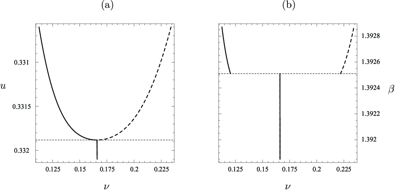
Figure 10: Structure of (a) the set ${\cal E}^{u,K}$ and (b) the set ${\cal E}_{\beta,K}$ for $K=1.0817$.

Figures 10(a) and 10(b) exhibit, for a range of values of $u$ and $\beta$, the structure of the set ${\cal E}^{u,K}$ of microcanonical equilibrium macrostates and the set ${\cal E}_{\beta,K}$ of canonical equilibrium macrostates for $K=1.0817$. This value of $K$ lies in the interval $(K_{\mbox{{\scriptsize\rm tri}}}^{\mbox{{\scriptsize\rm micro}}},K_{\mbox{{\scriptsize\rm tri}}}^{\mbox{{\scriptsize\rm canon}}})\approx(1.0813,1.0820)$. Each equilibrium macrostate in ${\cal E}^{u,K}$ and ${\cal E}_{\beta,K}$ is an empirical measure having the form

$$\nu=\nu_{1}\delta_{1}+\nu_{0}\delta_{0}+\nu_{-1}\delta_{-1}.$$

In both figures the solid and dashed curves can be taken to represent the components $\nu_{1}$ and $\nu_{-1}$. The components $\nu_{1}$ and $\nu_{-1}$ in the microcanonical ensemble are functions of $u$ [Fig. 10(a)] and in the canonical ensemble are functions of $\beta$ [Fig. 10(b)]. Figures 10(a) and 10(b) were taken from ETT .

Comparing the two figures reveals that the ensembles are nonequivalent for this value of $K$. Specifically, because of the discontinuous, first-order phase transition in the canonical ensemble, there exists a subset of $\mathcal{P}$ that is not realized by $\mathcal{E}_{\beta,K}$ for any $\beta>0$. On the other hand, since the set $\mathcal{E}^{u,K}$ of microcanonical equilibrium macrostates exhibits a continuous, second-order phase transition, the subset of $\mathcal{P}$ not realized canonically is realized microcanonically. As a result, there exists an inequivalence of ensembles at the level of equilibrium macrostates. The reader is referred to ETT for a more complete analysis of ensemble equivalence and nonequivalence for the BEG model.

VI Limit Theorems for the Total Spin with Respect to $P_{n,\beta,K}$

In Section 3.1, we rewrote the canonical ensemble $P_{n,\beta,K}$ in terms of the total spin $S_{n}$ and thus reduced the analysis of the set $\tilde{\mathcal{E}}_{\beta,K}$ of canonical equilibrium macrostates to that of a Curie-Weiss-type model. We end this paper with limit theorems for the $P_{n,\beta,K}$-distributions of appropriately scaled partial sums $S_{n}\doteq\sum_{j=1}^{n}\omega_{j}$. $S_{n}$ represents the total spin in the model. Since $S_{n}/n=\int_{\Lambda}y\,L_{n}(dy)$, the limit theorems for $S_{n}$ are also limit theorems for the empirical measures $L_{n}$. The new theorems follow from limit theorems for the Curie-Weiss model proved in EN and ENR .

Recall the function $G_{\beta,K}$ defined in (3.8) as

$$G_{\beta,K}(z)\doteq\beta Kz^{2}-c_{\beta}(2\beta Kz),$$ (6.1)

where $c_{\beta}$ is defined in (III.1). Proposition 3.4 characterizes the set of canonical equilibrium macrostates $\tilde{\mathcal{E}}_{\beta,K}$ by the formula

$$\tilde{\mathcal{E}}_{\beta,K}=\{z\in I\!\!R:z\mbox{ minimizes }G_{\beta,K}(z)\}.$$

In EN and ENR , it is proved that the limits in distribution of appropriately scaled partial sums $S_{n}$ in the Curie-Weiss model are determined by the minimum points of an analogue of $G_{\beta,K}$. As defined in (ENR, , eqn. (1.6)), this analogue is

$$G_{\beta}(z)=\frac{1}{2}\beta z^{2}-c_{\beta}(\beta z).$$

Carrying out a similar analysis of the minimum points of $G_{\beta,K}$ yields limit theorems for appropriately scaled partial sums $S_{n}$ for the BEG model. The limit theorems for the BEG model are proved exactly as in the Curie-Weiss case.

The function $G_{\beta,K}$ is real analytic. Hence for each global minimum point $\tilde{z}=\tilde{z}(\beta,K)\in\tilde{\mathcal{E}}_{\beta,K}$, there exists a positive integer $r=r(\tilde{z})$ such that $G_{\beta,K}^{(2r)}(\tilde{z})>0$ and

$$G_{\beta,K}(z)=G_{\beta,K}(\tilde{z})+\frac{G_{\beta,K}^{(2r)}(\tilde{z})(z-\tilde{z})^{2r}}{(2r)!}+O((z-\tilde{z})^{2r+1})\ \mbox{ as }z\longrightarrow\ \tilde{z}.$$

We call $r(\tilde{z})$ the type of the minimum point $\tilde{z}$. This concept is well-defined since $G_{\beta,K}$ is real analytic and $\tilde{z}$ is a global minimum point.

Because the limiting distributions for the scaled partial sums depend on the type of the minimum points $\tilde{z}$, we now classify each of the points in $\tilde{\mathcal{E}}_{\beta,K}$ by type. This is done in Theorem 6.1 for $\beta\leq\beta_{c}$ and $K>0$, in which case $\tilde{{\cal E}}_{\beta,K}$ exhibits a continuous bifurcation, and in Theorem 6.2 for $\beta>\beta_{c}$ and $K>0$, in which case $\tilde{{\cal E}}_{\beta,K}$ exhibits a discontinuous bifurcation. The associated limit theorems are given in Theorems 6.3 and 6.4. In all cases but one [Thm. 3.6(b)] the type of each of the minimum points is 1. When the type is 1, the associated limit theorems are central-limit-type theorems with scalings $n^{1/2}$. If $\tilde{{\cal E}}_{\beta,K}=\{0\}$, then $S_{n}/n^{1/2}$ converges in distribution to an appropriate normal random variable, and if $\tilde{{\cal E}}_{\beta,K}$ consists of multiple points, then $S_{n}/n^{1/2}$ satisfies a conditioned central-limit-type theorem. On the other hand, when $K=K_{c}^{2}(\beta)$, the type of the minimum point at 0 is $r=2$ or $r=3$ depending on whether $\beta<\beta_{c}$ or $\beta=\beta_{c}$. The associated limit theorems have non-central-limit scalings $n^{1-1/2r}$, and

$$P_{n,\beta,K}\{S_{n}/n^{1-1/2r}\in dx\}\Longrightarrow\mbox{const}\cdot\exp[-\mbox{const}\cdot x^{2r}]\,dx.$$

These non-classical limit theorems signal the onset of a phase transition (Ellis, , Sect. V.8).

We first consider $\beta\leq\beta_{c}\doteq\log 4$. According to Theorem 3.6, in this case there exists a critical value

$$K_{c}^{(2)}(\beta)\doteq\frac{1}{2\beta c_{\beta}^{\prime\prime}(0)}=\frac{1}{4\beta e^{-\beta}}+\frac{1}{2\beta}$$ (6.2)

with the following properties.

• For $K\leq K_{c}^{(2)}(\beta)$, $\tilde{\mathcal{E}}_{\beta,K}=\{0\}$.

• For $K>K_{c}^{(2)}(\beta)$, there exists $\tilde{z}=\tilde{z}(\beta,K)>0$ such that $\tilde{\mathcal{E}}_{\beta,K}=\{\pm\tilde{z}\}$.

The next theorem gives the type of each of these points in $\tilde{{\cal E}}_{\beta,K}$. The type is always $1$ except when $K=K_{c}^{(2)}(\beta)$; in this case the global minimum point at $0$ has type $r=2$ if $\beta<\beta_{c}$ and type $r=3$ if $\beta=\beta_{c}$.

Theorem 6.1

. Let $\beta\leq\beta_{c}=\log 4$ and define $K_{c}^{(2)}(\beta)$ by (6.2). The following conclusions hold.

(a) For $K<K_{c}^{(2)}(\beta)$, $z=0$ has type $r=1$.

(b) Let $K=K_{c}^{(2)}(\beta)$.

(i) For $\beta<\beta_{c}$, $z=0$ has type $r=2$.

(ii) For $\beta=\beta_{c}$, $z=0$ has type $r=3$.

(c) For $K>K_{c}^{(2)}(\beta)$ and each choice of sign, $z=\pm\tilde{z}(\beta,K)$ has type $r=1$.

Proof.  (a) By (6.2), we have

$$G_{\beta,K}^{\prime\prime}(0) = 2\beta K(1-2\beta Kc_{\beta}^{\prime\prime}(0))$$

$$= 2\beta K\left(1-\frac{K}{K_{c}^{(2)}(\beta)}\right).$$

Therefore, $K<K_{c}^{(2)}(\beta)$ implies that $G_{\beta,K}^{\prime\prime}(0)>0$ and thus that $z=0$ has type $r=1$.

(b) For $K=K_{c}^{(2)}(\beta)$, $G_{\beta,K}^{\prime\prime}(0)=0$. A simple calculation yields

$$G_{\beta,K}^{(4)}(0)=-(2\beta K)^{4}c_{\beta}^{(4)}(0)=-(2\beta K)^{4}\cdot\frac{2e^{-\beta}(1+2e^{-\beta})(1-2e^{-\beta}-8e^{-\beta})}{(1+e^{-\beta})^{4}}.$$ (6.3)

Therefore, for $\beta<\beta_{c}$, $G_{\beta,K}^{(4)}(0)>0$ and for $\beta=\beta_{c}$, $G_{\beta,K}^{(4)}(0)=0$. Computing the sixth derivative yields

$$G_{\beta_{c},K}^{(6)}(0)=2(2\beta K)^{6}/9.$$ (6.4)

As a result, $z=0$ has type 2 if $\beta<\beta_{c}$ and has type 3 if $\beta=\beta_{c}$.

(c) To prove that the symmetric minimum points $\pm\tilde{z}$ of $G_{\beta,K}$ each have type $r=1$, we employ the results of Lemma 2.3.5 in O . This lemma states the existence and uniqueness of nonzero global minimum points $\pm\tilde{w}=\pm\tilde{w}(\beta,K)$ of $F_{\beta,K}(w)\doteq w^{2}/4\beta K-c_{\beta}(w)$; $\tilde{w}$ is a global minimum point of $F_{\beta,K}$ if and only if $\tilde{z}\doteq\tilde{w}/2\beta K$ is a global minimum point of $G_{\beta,K}$. Lemma 2.3.5 in O also states that $F_{\beta,K}^{\prime\prime}(\tilde{w})>0$. Since $F_{\beta,K}^{\prime\prime}(\tilde{w})>0$ if and only if $G_{\beta,K}^{\prime\prime}(\tilde{z})>0$, the symmetry of $G_{\beta,K}$ allows us to conclude that for each choice of sign $\pm\tilde{z}$ has type $r=1$. This completes the proof.   

We next classify by type the points in $\tilde{\mathcal{E}}_{\beta,K}$ for $\beta>\beta_{c}$ and $K>0$. According to Theorem 3.7, there exists a critical value $K_{c}^{(1)}(\beta)$ with the following properties.

• For $K<K_{c}^{(1)}(\beta)$, $\tilde{\mathcal{E}}_{\beta,K}=\{0\}$.

• For $K=K_{c}^{(1)}(\beta)$, there exists $\tilde{z}=\tilde{z}(\beta,K)>0$ such that $\tilde{\mathcal{E}}_{\beta,K}=\{0,\pm\tilde{z}\}$.

• For $K>K_{c}^{(1)}(\beta)$, $\tilde{\mathcal{E}}_{\beta,K}=\{\pm\tilde{z}\}$.

The next theorem shows that the type of each of these points in ${\cal E}_{\beta,K}$ is $1$.

Theorem 6.2

. Let $\beta>\beta_{c}$ and $K>0$. The points in $\tilde{\mathcal{E}}_{\beta,K}$ all have type $r=1$.

Proof.  We first consider when $\tilde{{\cal E}}_{\beta,K}$ contains 0, in which case $K\leq K_{c}^{(1)}(\beta)$. Define $K_{2}\doteq 1/2\beta c_{\beta}^{\prime\prime}(0)$. It is proved in Lemma 2.3.15 in O that for $\beta>\beta_{c}$ we have $K_{c}^{(1)}(\beta)<K_{2}$. Since

$$G_{\beta,K}^{\prime\prime}(0) = 2\beta K(1-2\beta Kc_{\beta}^{\prime\prime}(0))$$

$$= 2\beta K\left(1-\frac{K}{K_{2}}\right),$$

it follows that whenever $K\leq K_{c}^{(1)}(\beta)$, $1>K/K_{2}$ and thus $G_{\beta,K}^{\prime\prime}(0)>0.$ We conclude that the minimum point of $G_{\beta,K}$ at $z=0$ has type $r=1$, as claimed.

For $K\geq K_{c}^{(1)}(\beta)$, $\tilde{{\cal E}}_{\beta,K}$ also contains the symmetric, nonzero minimum points $\pm\tilde{z}$ of $G_{\beta,K}$. We prove that each of these points has type $r=1$, employing the results of Lemma 2.3.11 in O . This lemma states the existence and uniqueness of nonzero global minimum points $\pm\tilde{w}=\pm\tilde{w}(\beta,K)$ of the function $F_{\beta,K}(w)\doteq w^{2}/4\beta K-c_{\beta}(w)$; $\tilde{w}$ is a global minimum point of $F_{\beta,K}$ if and only if $\tilde{z}\doteq\tilde{w}/2\beta K$ is a global minimum point of $G_{\beta,K}$. Furthermore, Lemma 2.3.11 states that $F_{\beta,K}^{\prime\prime}(\tilde{w})>0$. Since $F_{\beta,K}^{\prime\prime}(\tilde{w})>0$ if and only if $G_{\beta,K}^{\prime\prime}(\tilde{z})>0$, the symmetry of $G_{\beta,K}$ allows us to conclude that for each choice of sign $\pm\tilde{z}$ has type $r=1$. This completes the proof.   

We now state the limit theorems for the $P_{n,\beta,K}$-distributions for appropriately scaled partial sums $S_{n}$. The first, Theorem 6.3, states limit theorems that are valid when $G_{\beta,K}$ has a unique global minimum point at $z=0$. This is the case for $\beta\leq\beta_{c}$, $K\leq K_{c}^{(2)}(\beta)$ [Thm. 3.6(a)] and for $\beta>\beta_{c}$, $K<K_{c}^{(1)}(\beta)$ [Thm. 3.7(a)]. The second, Theorem 6.4, states conditioned limit theorems that are valid when $G_{\beta,K}$ has multiple global minimum points. Because Theorems 6.3 and 6.4 are immediate applications of Theorems 2.1 of EN and 2.4 of ENR , respectively, we state them here without proof.

In Theorem 6.3 $f_{0,\sigma^{2}}$ denotes the density of an $N(0,\sigma^{2})$ random variable with

$$\sigma^{2}\doteq\frac{2\beta Kc_{\beta}^{\prime\prime}(0)}{G_{\beta,K}^{\prime\prime}(0)}.$$ (6.6)

When the type of the minimum point at $0$ is $r=1$, $\sigma^{2}>0$ because in this case $G_{\beta,K}^{\prime\prime}(0)>0$ and in general $c_{\beta}^{\prime\prime}(0)>0$. If $f$ is a nonnegative, integrable function on $I\!\!R$, then for $r=1$, 2, or 3 we write

$$P_{n,\beta,K}\{S_{n}/n^{1-1/2r}\in dx\}\Longrightarrow f(x)\,dx$$

to mean that as $n\rightarrow\infty$ the $P_{n,\beta,K}$-distributions of $S_{n}/n^{1-1/2r}$ converge weakly to a distribution with density proportional to $f$. When $r=1$, $f=f_{0,\sigma^{2}}$, and the limit is a central-limit-type theorem with scaling $n^{1/2}$. When $r=2$ or 3, the limits involve the nonclassical scaling $n^{3/4}$ or $n^{5/6}$, respectively, and the $P_{n,\beta,K}$-distributions of the scaled random variables converge weakly to a distribution having a density proportional to $\exp[-\mbox{const}\cdot z^{4}]$ or $\exp[-\mbox{const}\cdot z^{6}]$.

Theorem 6.3

. Suppose that $\tilde{\mathcal{E}}_{\beta,K}=\{0\}$ and let $r$ be the type of the point $z=0$ as given in Theorems 6.1 and 6.2. With $\sigma^{2}$ the positive quantity defined in (6.6), as $n\rightarrow\infty$

$$P_{n,\beta,K}\!\left\{\frac{S_{n}}{n^{1-1/2r}}\in dx\right\}\Longrightarrow\left\{\begin{array}[]{ll}f_{0,\sigma^{2}}(x)\,dx&\mbox{ for }r=1\\ \exp(-G_{\beta,K}^{(2r)}(0)x^{2r}/(2r)!)\,dx&\mbox{ for }r=2\mbox{ or }r=3.\end{array}\right.$$

When $r=2$ [$K=K_{c}^{(2)}(\beta)$, $\beta<\beta_{c}$], $G_{\beta,K}^{(4)}(0)$ is given by (6.3), and when $r=3$ [$K=K_{c}^{(2)}(\beta)$, $\beta=\beta_{c}$], $G_{\beta,K}^{(6)}(0)=2(2\beta K)^{6}/9$.

Our last theorem states conditioned limit theorems that are valid when $G_{\beta,K}$ has multiple minimum points. This holds in three cases: (1) when $\beta\leq\beta_{c}$ and $K>K_{c}^{(2)}(\beta)$, in which case the minimum points are $\pm\tilde{z}(\beta,K)$ with $\tilde{z}(\beta,K)>0$ [Thm. 3.6(b)]; (2) when $\beta=\beta_{c}$ and $K=K_{c}^{(1)}(\beta)$, in which case the minimum points are $0,\pm\tilde{z}(\beta,K)$ with $\tilde{z}(\beta,K)>0$ [Thm. 3.7(b)]; (3) when $\beta=\beta_{c}$ and $K>K_{c}^{(1)}(\beta)$, in which case the minimum points are $\pm\tilde{z}(\beta,K)$ with $\tilde{z}(\beta,K)>0$ [Thm. 3.7(c)]. In each case in which $G_{\beta,K}$ has multiple minimum points, Theorems 6.1and 6.2 states that all the minimum points have type $r=1$. Hence, if we denote the minimum points by ${z}_{j}$ for $j=1,2$ or for $j=1,2,3$, then for each $j$ we have $G_{\beta,K}^{\prime\prime}({z}_{j})>0$. Defining

$$\sigma_{j}^{2}\doteq\frac{2\beta Kc_{\beta}^{\prime\prime}(2\beta K{z}_{j})}{G_{\beta,K}^{\prime\prime}({z}_{j})},$$ (6.7)

we see that $\sigma_{j}^{2}>0$.

Theorem 6.4

. Suppose that $\tilde{\mathcal{E}}_{\beta,K}=\{{z}_{1},...,{z}_{m}\}$ for $m=2$ or 3. For each $j=1,\ldots,m$ we let $f_{0,\sigma_{j}^{2}}$ be the density of an $N(0,\sigma_{j}^{2})$ random variable, where $\sigma_{j}^{2}$ is the positive quantity defined in (6.7). Then there exists $A=A({z}_{j})>0$ such that for any $a\in(0,A)$

$$P_{n,\beta,K}\!\left\{\frac{S_{n}-nz_{j}}{n^{1/2}}\in dx\left|\,\frac{S_{n}}{n}\in[{z}_{j}-a,{z}_{j}+a]\right.\right\}\Longrightarrow f_{0,\sigma_{j}}(x)\,dx\mbox{ as }n\rightarrow\infty.$$

This completes our study of the limits for the $P_{n,\beta,K}$-distributions of appropriately scaled partial sums $S_{n}\doteq\sum_{j=1}^{n}\omega_{j}$.

References

• (1) J. Barré, D. Mukamel, and S. Ruffo. Inequivalence of ensembles in a system with long-range interactions. Phys. Rev. Lett 87:030601 (2001).
• (2) J. Barré, D. Mukamel, and S. Ruffo. Ensemble inequivalence in mean-field models of magnetism. In T. Dauxois, S. Ruffo, E. Arimondo, and M. Wilkens, editors. Dynamics and Thermodynamics of Systems with Long Range Interactions, pages 45–67. Volume 602 of Lecture Notes in Physics. New York: Springer-Verlag, 2002.
• (3) M. Blume, V. J. Emery, and R. B. Griffiths. Ising model for the $\lambda$ transition and phase separation in $\mbox{He}^{3}$-$\mbox{He}^{4}$ mixtures. Phys. Rev. A 4:1071–1077 (1971).
• (4) M. Costeniuc, R. S. Ellis, and H. Touchette. Complete analysis of phase transitions and ensemble equivalence for the Curie-Weiss-Potts model. In preparation, 2004.
• (5) T. Eisele and R. S. Ellis. Symmetry breaking and random waves for magnetic systems on a circle. Z. Wahrsch. verw. Geb. 63:297–348 (1983).
• (6) R. S. Ellis. Entropy. Large Deviations and Statistical Mechanics. New York: Springer-Verlag, 1985.
• (7) R. S. Ellis, K. Haven, and B. Turkington. Large deviation principles and complete equivalence and nonequivalence results for pure and mixed ensembles. J. Stat. Phys. 101:999–1064 (2000).
• (8) R. S. Ellis, J. L. Monroe, and C. M. Newman. The GHS and other correlation inequalities for a class of even ferromagnets. Commun. Math. Phys. 46:167–182 (1976).
• (9) R. S. Ellis and C. M. Newman. Limit theorems for sums of dependent random variables occurring in statistical mechanics. Z. Wahrsch. verw. Geb. 44:117-139 (1979)
• (10) R. S. Ellis, C. M. Newman, and J. S. Rosen. Limit theorems for sums of dependent random variables occurring in statistical mechanics, II: conditioning, multiple phases, and metastability. Z. Wahrsch. verw. Gebiete 51:153–169 (1980)
• (11) R. S. Ellis, C. M. Newman, and M. R. O’Connell. The GHS inequality for a large external field. J. Stat. Phys. 26:37–52 (1981).
• (12) R. S. Ellis, H. Touchette, and B. Turkington. Thermodynamic verses statistical nonequivalence of ensembles for the mean-field Blume-Emery-Griffiths model. Physica A 335:518- 538 (2004).
• (13) W. Hoston and A. N. Berker. Multicritical phase diagrams of the Blume-Emery-Griffiths model with repulsive biquadratic coupling. Phys. Rev. Lett 67:1027–1030 (1991).
• (14) S. A. Kivelson, V. J. Emery, and H. Q. Lin. Doped antiferromagnets in the weak-hopping limit. Phys. Rev. B 42:6523–6530 (1990).
• (15) J. Lajzerowicz and J. Sivardière. Spin-1 lattice-gas model. I. Condensation and solidification of a simple fluid. Phys. Rev. A 11:2079–2089 (1975).
• (16) K. E. Newman and J. D. Dow. Zinc-blende-diamond order-disorder transition in metastable crystalline (GzAs)1-xGe2x alloys. Phys. Rev. B 27:7495–7508 (1983).
• (17) B. Nienhuis, A. N. Berker, E. K. Riedel and M. Schick. First- and second-order phase transitions in Potts models: Renormalization-group solution. Phys. Rev. Lett 43:737–740 (1979).
• (18) P. Otto. Study of Equilibrium Macrostates for Two Models in Statistical Mechanics. Ph.D. dissertation, University of Massachusetts Amherst (2004). An online copy of this dissertation is available at
http://www.math.umass.edu/~ rsellis/pdf-files/Otto-thesis.pdf.
• (19) R. T. Rockafellar. Convex Analysis. Princeton, NJ: Princeton Univ. Press, 1970.
• (20) M. Schick and W. -H. Shih. Spin-1 model of a microemulsion. Phys. Rev. B 34:1797–1801 (1986).
• (21) J. Sivardière and J. Lajzerowicz. Spin-1 lattice-gas model. II. Condensation and phase separation in a binary fluid. Phys. Rev. A 11:2090–2100 (1975).
• (22) J. Sivardière and J. Lajzerowicz. Spin-1 lattice-gas model. III. Tricritical points in binary and ternary fluids. Phys. Rev. A 11:2101–2110 (1975).