Random Deposition Model with a Constant Capture Length

Abstract

We introduce a sequential model for the deposition and aggregation of particles in the submonolayer regime. Once a particle has been randomly deposited on the substrate, it sticks to the closest atom or island within a distance $\ell$, otherwise it sticks to the deposition site. We study this model both numerically and analytically in one dimension. A clear comprehension of its statistical properties is provided, thanks to capture equations and to the analysis of the island-island distance distribution.

1 Introduction

The morphology of a system growing by deposition and aggregation of particles [1] depends on several factors and it is not exaggerated to say that a detailed description would require a theory, or at least a model, for each different physical system. In spite of this, the use of simple and general models for studying growth processes is widespread. This is justified by two big reasons: First, such models allow to study large-scale features which are common to different physical systems; Second, they allow to connect apparently different phenomena.

In the following we are referring to the growth process of a crystal surface by molecular beam epitaxy [2], with a special interest in the submonolayer regime [3], where only a fraction of a monolayer has been deposited. With these caveats in mind, a simple and very popular model for the growth process [2] accounts for random deposition of atoms and their thermally activated diffusion till they meet irreversibly another atom (nucleation) or island (aggregation). The system is therefore made up of diffusing particles (adatoms) and still islands. New atoms, which are continuously provided by deposition, can not leave the surface, because evaporation is forbidden at low temperature. Hereafter, this model will be called ‘full diffusion’ model.

The diffusion length, $\ell_{\hbox{\tiny D}}$, is an important quantity. It measures the typical (linear) distance walked by an adatom before being incorporated [4]. It depends on the deposition rate, $F$, and the hopping rate, $h$, through the relation $\ell_{\hbox{\tiny D}}\sim(h/F)^{1/\gamma}$, with $\gamma=2(d^{*}+1)$, where $d^{*}$ is the spatial dimension of the system. Once an atom has been deposited it visits a region of linear size $\ell_{\hbox{\tiny D}}$ and sticks inside that region after a time $\tau_{\hbox{\tiny D}}\sim\ell_{\hbox{\tiny D}}^{2}/h$. The probability that another deposition occurs during this time in that region of size $\ell_{\hbox{\tiny D}}$ is

$$F\tau_{\hbox{\tiny D}}\ell_{\hbox{\tiny D}}^{d^{*}}\sim(F/h)\ell_{\hbox{\tiny D}}^{2+d^{*}}\sim\ell_{\hbox{\tiny D}}^{2+d^{*}-\gamma}\sim\ell_{\hbox{\tiny D}}^{-d^{*}}\,.$$ (1)

Since $\ell_{\hbox{\tiny D}}\gg 1$ such probability is very small, meaning that the sticking process of a new adatom is not influenced by atoms deposited later on. These arguments lead us to consider an even simplified model, which we are now going to describe.

Once an atom has been deposited, it immediately searches the surroundings for another atom or an island. If it exists, it sticks to it, otherwise it sticks to the deposition site. Next, another atom is deposited. The search will be implemented deterministically through a capture area: the newly deposited atom (adatom in the following) looks for the closest atom/island within a distance $\ell$. Each adatom will therefore attach to an existing atom/island or it will stick to the deposition site and collect atoms deposited later on in its capture area. It is to be noted that in the present model an adatom moves around only at the time of deposition, but never afterwards. It is also important to stress that the size of the effective capture area reduces in the course of time, if newly deposited atoms have their own capture area overlapping with it. The reason is that particles at a distance $d$, with $\ell<d<2\ell$, do not capture each other, but their capture areas overlap, and their capture distances along the joining line are reduced to $d/2$.

We are going to study the above model, both numerically and analytically, in one spatial dimension ($d^{*}=1$). This choice is due to the possibility to provide a full theoretical comprehension of numerical results, using two main analytic tools: capture equations and the analysis of the island-island distance distribution.

In the literature of submonolayer deposition, two models for representing islands are usually found: ‘extended-islands’ and ‘point-islands’. In the former case, the physical size of an island increases proportionally to the number of adatoms attached to it and its shape depends on additional factors. In the latter case, islands have a physical size equal to a lattice site whatever is the number of atoms they are made up. The two models are statistically equivalent at small coverage (see next Section). We will use a ‘point-island’ model because of its simplicity.

A last remark relates to the physical interpretation of the capture length and to the novelty of our model. If we refer to a system which displays a thermally activated diffusion process, our capture length can be read as an effective way to implement it. The idea is not new: it has been used, e.g., by Michael Biehl, Wolfgang Kinzel and coworkers in several papers [5] for studying multilayer growth and it is related to the model of random deposition with surface relaxation [6]. However, we are not aware of the application of the idea of capture length to study the submonolayer regime. On the other hand, the capture length may represent nonthermal post deposition processes, as found, e.g., during the adsorption of rare gas atoms on metal surfaces [7].

This paper has three Sections, beyond the present Introduction. In the next Section we provide a summary of the main numerical results, while in Section 3 we derive the analytical results and compare them to numerics. In the final Section we discuss the hypotheses underlying our model and suggest a possible interpolation between our model and the ‘full diffusion’ model.

Some remarks on notations are in order. In the analytical calculations we generally use ‘dimensional’ quantities, for example for the distance $d$ between islands. However, when we display numerical results and compare them with analytics it may be useful to use reduce variables, for example $x=d/\ell$. In order to avoid any possible misunderstanding, we say that $d,\bar{d},\bar{d}_{\infty},d_{nn},d_{nnn},d_{l},d_{r},y$ are all dimensional distances. In particular, $\bar{d}$ is the average distance between neighbouring islands and $\bar{d}_{\infty}$ is its asymptotic value for large coverage (i.e., for large deposition time). The only adimensional distances that are used throughout the paper are $x$ and $\tilde{d}=\bar{d}_{\infty}/\ell$.

Finally, two probability distributions for the distance will be introduced, $P_{1}$ and $P_{2}$. They refer to the distance between first (nn) and second (nnn) nearest neighbouring islands, respectively.

2 Numerical Simulation

Our model is defined as follows. We choose randomly a lattice site and check if some atoms or islands exist within a distance $\ell$. If they exist, the newly deposited atom sticks to the closest atom/island, otherwise it sticks permanently to the deposition site. When an atom sticks to another atom, we get a new island.

The model has two main features: it is a sequential model and random deposition is the only source of noise. If $N_{a}$ atoms are deposited on a substrate of $L$ sites, the ratio $\theta=N_{a}/L$ defines the coverage $\theta$, which is also equal to the product of the deposition rate and the deposition time, $\theta=Ft$. The statistical properties of the model depend on the product between the capture area $c=2\ell+1$ and $\theta$: this product is the average number of particles deposited in the area $c$. All simulations have been done for $\ell\geq 10$, so that in the following we can write $c\simeq 2\ell$ and introduce the parameter $p=\theta\ell$. Point-island and extended-island models have the same properties at small coverage, let’s say $\theta<0.2$. This condition can be satisfied at any $p$, if the capture length is large enough, $\ell>5p$.

Let us now give a qualitative description of the growth morphology followed by a summary of numerical results. Since all quantities depend on $p=\theta\ell$ only, we can think to keep $\ell$ fixed and vary $\theta$ or the other way round. For pedagogical reasons we are describing the growth morphology with increasing $\theta$.

At the very beginning, deposited atoms do not interact and each atom or island grows in size according to the number of particles deposited in its capture area $c=2\ell$. The average distance between atoms or islands is very large. With increasing $\theta$, atoms or islands densities increase and their capture areas start to overlap. From then on the growth processes of different islands are no more independent. The average distance is now between $\ell$ and $2\ell$. At large $\theta$, almost all neighbouring islands have distances $d<2\ell$. The majority of islands therefore increases in size according to the number of particles deposited in a capture area equal to half the distance with the left and right neighbours. Sometimes two neighbouring islands have a distance $d>2\ell$ and the interval may be empty or contain one atom. Densities of atoms and islands change because empty intervals are filled by atoms and atoms are transformed into islands. Let us now sum up the numerical results with the aid of the figures.

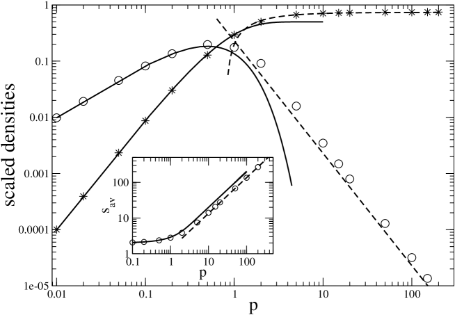
Figure 1: Numerical (symbols) and analytical (lines) results for the adatom (circles) and island (stars) densities. At small $p$ (full lines) adatom density varies as $\tilde{n}_{1}=p\exp(-2p)$ and island density varies as $\tilde{n}_{is}=\frac{1}{2}-(p+\frac{1}{2})\exp(-2p)$. At large $p$ (dashed lines), $\tilde{n}_{1}$ decays as $1/p^{2}$ and and $\tilde{n}_{is}$ approaches the asymptotic value $\tilde{n}_{is}^{\infty}$ as $1/p$ (see Eqs.(28,29)). Inset: The average size of islands as a function of $p$. Full line: small $p$ approximation. Dashed line: large $p$ approximation ($s_{av}=\tilde{d}p$). All analytical results do not contain any fitting parameter.

Fig. 1 summarizes all the main average quantities: the densities of atoms (circles) and islands (stars) in the main figure and the average size of islands in the inset. At small $p$, the density of atoms ($\tilde{n}_{1}$) increases linearly, of course, and the density of islands ($\tilde{n}_{is}$) increases quadratically (the tilde over a density means a reduced density, $\tilde{n}_{[]}=\ell n_{[]}$, see next Section). This behaviour is related to the specific features of the nucleation process in the present model, which is due to the deposition of an atom in the capture area of an existing atom and it is not mediated by surface diffusion, as in epitaxial growth. In the latter case $\tilde{n}_{is}$ increases with $\theta$ (i.e., with $p$) as $\tilde{n}_{is}\approx\theta^{\chi}$, with an exponent [8] $\chi=3$ in two dimensions. Mean-field rate equations predict the same exponent in one dimension as well, but in this case the assumption $d\tilde{n}_{is}/d\theta\approx\tilde{n}_{1}^{2}$ is wrong. The correct theory for nucleation on top of a terrace [9] suggests $\chi=\frac{5}{2}$.

At large $p$, $\tilde{n}_{is}$ saturates but does not decrease because coalescence of islands is not possible in a point-island model. The limiting value, $\tilde{n}_{is}^{\infty}$, is related to the reduced asymptotic average distance between islands, $\tilde{d}=\bar{d}_{\infty}/\ell$, by the trivial relation $\tilde{n}_{is}^{\infty}=1/\tilde{d}$. Island density converges to $\tilde{n}_{is}^{\infty}$ as $1/p$, while adatom density decays as $1/p^{2}$. These behaviours (see next Section) are due to the existence of intervals slightly larger than $2\ell$, which are ‘filled’ by an adatom, which is subsequently transformed in a island. The probabilities of the two processes differ: filling an interval $d\apprge 2\ell$ with an adatom requires deposition on a small region of size $d-2\ell$, while deposition on a region of size $\bar{d}_{\infty}$ is enough to make an island from an adatom. The process (adatom) $\to$ (island) is therefore quicker than the creation of new adatoms: this is the reason why $\tilde{n}_{1}$ decays more rapidly than $\tilde{n}_{is}$ converges to $\tilde{n}_{is}^{\infty}$. A quantitative, more rigorous analysis can be found in Section 3.3.

The inset of Fig. 1 gives the average size of islands, $s_{av}$. It is of order two for small $p$. At large $p$, deposited atoms are shared among existing islands, and $s_{av}$ increases linearly with $\theta$, i.e. with $p$.

Figure 2: The size distribution of islands for different values of $p$ (Main: $p=0.2,0.5,1$; Inset: $p=2,5$). Symbols: numerical results. Lines: analytical results according to the small $p$ approximation, Eq. (6).

Fig. 2 and Fig. 3 plot the size distribution of islands, at small (Fig. 2) and large (Fig. 3) $p$, respectively. At small $p$, when different islands are almost independent, the size distribution is expected to follow a Poisson distribution: this is confirmed by lines, which reproduce well numerical data (symbols) till $p\apprle 2$. At large $p$ an island grows in size because it collects atoms deposited in a region of size $\frac{1}{2}(d_{l}+d_{r})$, where $d_{l,r}$ are the distances to the nearest left and right neighbour. In this regime, the size distribution is therefore strictly related to the distance distribution between second nearest neighbouring (nnn) islands: this is proved in Fig. 3 by comparing the two (rescaled) distributions, plotted as full line and dashed line, respectively. The dotted line is the analytical nnn distance distribution ($P_{2}$), as derived from the island-island distance ditribution ($P_{1}$) under the assumption that there is no correlation between neighbouring distances (see the discussion in the next Section).

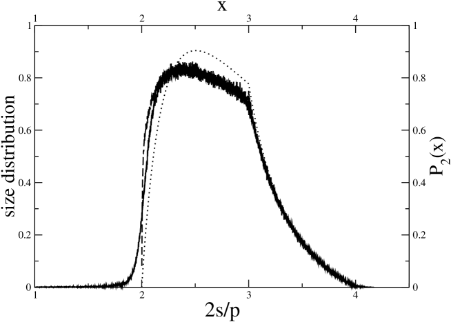
Figure 3: Numerical results for the size distribution (full line), as a function of $2s/p$. Distance distribution between next-nearest-neighbouring islands: numerical (dashed line) and analytical (dotted line) results ($x=d_{nnn}/\ell$).

The previous discussion shows that the distance distribution plays an important role to understand the statistical properties of the model. In Fig. 4a we report the distribution $P_{1}(x)$ of the normalized nn distance $x=d/\ell$, for several values of $p$ (note the log-scale on the $y$ axis). Distances smaller than one (i.e., $d<\ell$) are forbidden, of course. Two regimes are clearly visible, for $x$ smaller and larger than $2$. The reason is straightforward: the capture areas of two neighbouring islands at distance $x<2$ overlap, while they do not if $x>2$. This implies that new islands can nucleate in between only in the latter case.

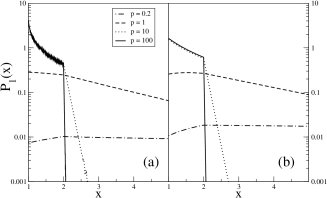
Figure 4: Simulation (a) and theory (b) for the island-island distance distribution, as a function of $x=d/\ell$, for $p=0.2,1,10,100$.

For $x>2$, $P_{1}(x)$ decays exponentially, $P_{1}(x)\sim\exp(-\alpha x)$ with a prefactor $\alpha$ depending on $p$ (see Fig. 5). At smaller distances, $x<2$, $P_{1}(x)$ depends algebrically on $x$. Furthermore, it is an increasing function at small $p$ and a decreasing one at large $p$. For very large $p$, it converges to a limiting shape (see Fig. 6), except for $x$ very close to one.

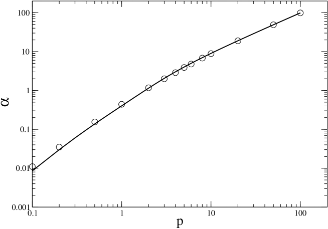
Figure 5: Numerical (circles) and analytical (full line) results for the prefactor $\alpha$, which characterizes the exponential decreasing of the distance distribution $P_{1}(x)$, for $x=d/\ell>2$, $P_{1}(x)\sim\exp(-\alpha(p)x)$. $\alpha=p^{2}$ for small $p$ and $\alpha=p-1$ for large $p$.

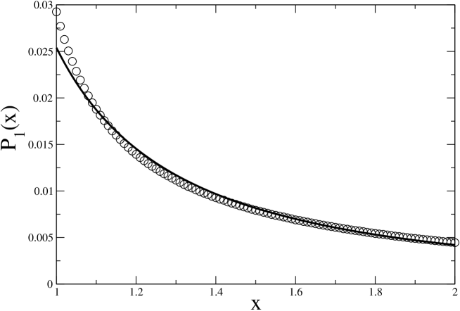
Figure 6: Numerical (circles) and analytical (full line) results for the ‘asymptotic’ ($p=20$) distance distribution $P_{1}(x)$ in the interval $1<x<2$, i.e. $\ell<d<2\ell$.

3 Quantitative Analysis

3.1 Densities and size distributions for small $p$

In the following $n_{1}$ is the density of adatoms (adatoms per lattice site), $n_{s}$ ($s\geq 2$) is the density of islands of size $s$, and $n_{is}=\sum_{s\geq 2}n_{s}$ is the total density of islands. The quantities $\tilde{n}_{[]}=\ell n_{[]}$ are the ‘reduced’ densities and they mean the number of adatoms/islands per capture length. In the limit of small $p$ deposited particles do not interact because their distance is larger than $2\ell$ and each adatom or island has a capture area equal to $2\ell$. In this limit it is possible to write down the following capture equations ($p=\theta\ell$):

$${d\tilde{n}_{1}\over dp} = 1-2(\tilde{n}_{is}+2\tilde{n}_{1})$$ (2)

$${d\tilde{n}_{is}\over dp} = 2\tilde{n}_{1}$$ (3)

which can be easily solved, giving

$$\tilde{n}_{1}=p\exp(-2p)\,,~{}~{}~{}~{}\tilde{n}_{is}=\hbox{${1\over 2}$}-(p+\hbox{${1\over 2}$})\exp(-2p)\,.$$ (4)

These expressions, that are consistent for any $p$, are reported in Fig. 1 as full lines and compared with numerical results (symbols). Comparison is almost perfect till $p\approx 1$. For larger values overlapping of capture areas is relevant and the above approximation is no more valid. The main defect of (4), due to the assumption of a constant capture area, is that $\tilde{n}_{1}$ and $\frac{1}{2}-\tilde{n}_{is}=\tilde{n}_{is}^{\infty}-\tilde{n}_{is}$ decrease exponentially for $p\to\infty$, instead of that in a power law. The limit of large $p$ will be treated in Section 3.3.

The equations for the density evolutions of islands of any size $s\geq 2$ are

$${d\tilde{n}_{s}\over dp}=2(\tilde{n}_{s-1}-\tilde{n}_{s})$$ (5)

and they can be solved recursively,

$$\tilde{n}_{s}={1\over 2}{(2p)^{s}\over s!}\exp(-2p)~{}~{}~{}s\geq 1$$ (6)

showing that at small coverage the size distribution is Poisson-like. In Fig. 2 we compare the above analytical expressions with numerical results: they match very well till $p\approx 1$. The average size $s_{av}$ of islands ($s\geq 2$) is calculated as

$$s_{av}=\frac{\sum_{s=2}^{\infty}s\tilde{n}_{s}}{\tilde{n}_{is}}=2p{\exp(2p)-1\over\exp(2p)-(1+2p)}\,.$$ (7)

This small $p$ approximation for $s_{av}$ is reported in the inset of Fig. 1 as a full line. It also reproduces the correct linear behaviour at large $p$ ($s_{av}=ap$), but with a wrong factor $a$. The reason is that the small $p$ approximation gives an asymptotic value for the island density, $\tilde{n}_{is}^{\infty}=\frac{1}{2}$, which is smaller than the actual value (compare stars and full line in Fig. 1); therefore $a=1/\tilde{n}_{is}^{\infty}$ is overestimated.

Finally, expression (6) for $\tilde{n}_{s}$ might be slightly improved for $p\apprge 1$ by replacing $(2p)$ with a parameter $\lambda$ in Eqs. (6) and (7). This parameter should be determined by Eq. (7) using the actual numerical value for $s_{av}$.

3.2 Island-Island distance distribution

In Fig. 4a we plot the distribution of distances between nearest neighboring islands as a function of the ‘reduced’ distance $x=d/\ell$. The existence of two regimes separated at $x=2$ is due to the possibility of creating a new island within an interval, only if $d>2\ell$. The weight of the two regimes changes with $p$, because the fraction of distances $d<2\ell$ increases from zero to one as $p$ increases.

For $x>2$ the distribution has an exponential behaviour, $P_{1}(x)\sim\exp(-\alpha x)$. In this regime the capture areas of two neighbouring islands do not overlap and $P_{1}(x)$ is just the probability that no island nucleation occurs in time $\theta$ in the interval of size $d$ between the two islands[10]. If $\omega(t)$ is the nucleation probability per unit time and unit length, at time $t$, neglecting correlations of nucleation events we obtain

$$P_{1}(x)=\exp\left[-d\hskip-2.84544pt\int_{0}^{\theta}\hskip-2.84544ptdt\,\omega(t)\right]\,.$$ (8)

Nucleation occurs when an atom is deposited in the capture area of an already existing atom. If a deposition event increases the (total) capture area by $\Delta$, then $d\omega/dt=(1-\omega)\Delta$, i.e. $\omega(t)=1-\exp(-\Delta t)$. Inserting the last expression in (8) and introducing $\delta=\Delta/\ell$, we obtain

$$\alpha(p) = \int_{0}^{p}d\tau(1-e^{-\delta\tau})$$ (9)

$$= p-(1-e^{-\delta p})/\delta\,.$$ (10)

In fact, the quantity $\delta$ is not constant, but it decreases in time, i.e. with $p$, being equal to two for $p\to 0$. In Fig. 5 we compare numerical data for $\alpha$ with Eq. (10), assuming $\delta=1+\exp(-p)$, which gives the correct limits $\delta\approx 2$ for small $p$ and $\delta\approx 1$ for large $p$.[11] The agreement is fairly good.

If $x<2$ the determination of $P_{1}(x)$ is more difficult because of the ‘interaction’ between the capture zones of the two neighbouring islands. The existence of two islands in $y=0$ and $y=d$ after a time $\theta$ can be depicted as follows. If we assume that the (first) atom in zero is deposited at time $t_{1}$ and the atom in $d$ is deposited at time $t_{2}>t_{1}$, we require that no deposition takes place in a region $(d+2\ell)$ during time $t_{1}$, no deposition in a region $d$ between $t_{1}$ and $t_{2}$, at least one deposition in $2\ell$ between $t_{1}$ and $\theta$, at least one deposition in $d$ between $t_{2}$ and $\theta$[12]. Integrating over $t_{1}$ and $t_{2}$ the product of all the above probabilities provides $P_{1}(d)$ in the hypothesis that neighbouring intervals have no influence,

$$P_{1}(d) = \int_{0}^{\theta}dt_{1}\exp(-2\ell t_{1})\int_{t_{1}}^{\theta}dt_{2}\exp(-dt_{2})\times$$ (11)

$$\times[1-\exp(-d(\theta-t_{2}))][1-\exp(-2\ell(\theta-t_{1}))]$$

$$= \exp(-(d+2\ell)\theta)[I_{1}/d-I_{2}]$$

where

$$I_{1} = {\exp((2\ell+d)\theta)-1\over 2\ell+d}-{\exp(2\ell\theta)-1\over 2\ell}-{\exp(d\theta)-1\over d}+\theta$$ (12)

$$I_{2} = \left(2\ell\theta\exp(2\ell\theta)-\exp(2\ell\theta)-2\ell^{2}\theta^{2}+1\right)/4\ell^{2}\,.$$ (13)

Prefactors are missing in Eqs. (8,11). They are determined imposing the continuity of $P_{1}(d)$ in $d=2\ell$ and its normalization in $(\ell,\infty)$. The result of this procedure is shown in Fig. 4b, whose qualitative comparison with simulation results (Fig. 4a) is rather satisfying. The quantitative comparison is good for small $p$, but is not for large $p$. The reason is simple: for large $p$, the average distance $\bar{d}$ between islands is smaller than $2\ell$, which means that neglecting the left and right neighbours of the two islands located in $y=0$ and $y=d$ is no more correct. It is possible to take them into account in a ‘mean field approximation’, by assuming the existence of such neighbours at a fixed distance $\bar{d}$. At small $p$, $\bar{d}>2\ell$ and this refinement is inessential, but for large $p$ is relevant.

The calculation proceeds along the same lines leading to (11) with the difference that now capture areas are limited by the presence of two additional islands in $y=-\bar{d}$ and $y=d+\bar{d}$. If we limit ourselves to the case $p\gg 1$, the refined procedure gives

$$P_{1}(d)={P_{0}\over(d+\bar{d}_{\infty}-2\ell)(d+2\bar{d}_{\infty}-2\ell)}\,,$$ (14)

where $P_{0}$ and $\bar{d}_{\infty}$ should be determined self-consistently through the conditions

$$\int_{\ell}^{2\ell}dyP_{1}(y)=1~{}~{}~{},~{}~{}~{}\int_{\ell}^{2\ell}dyyP_{1}(y)=\bar{d}_{\infty}\,.$$ (15)

In Fig. 6 we compare the analytical and numerical results for $P_{1}(d)$ in the regime $d<2\ell$, using the reduced distance $x=d/\ell$. A couple of remarks are in order. First, the analytical curve has no fitting parameter. Second, the inverse of the reduced average distance $\tilde{d}=\bar{d}_{\infty}/\ell$ has the value $1/\tilde{d}=0.738$, determined self-consistently from the above procedure. This value agrees very well with the asymptotic island density for large $p$, $\tilde{n}_{is}^{\infty}\approx 0.75$. The value of $\tilde{d}$ also allows to draw the dashed line in the inset of Fig. 1, which gives the theoretical prediction $s_{av}=\tilde{d}p$ for the average size of islands at large $p$.

A final comment concerns the shape of $P_{1}(x)$ for $x<2$, in the limit $p\to\infty$. The curve with circles in Fig. 6 refers to $p=20$. Numerical results show that a limiting shape does exist for $x\apprge 1.1$, while $P_{1}(1)$ seems to have a logarithmic divergence. This behaviour is due to distance-distance correlations which are not taken into account by the mean-field approximation leading to Eq. (14).

3.3 Size distributions and adatom/island densities for large $p$

Fig. 3 shows that the asymptotic size distribution $\tilde{n}_{s}$ (full line) agrees well with the distance distribution $P_{2}(x)$ (dashed line) between next-nearest-neighbouring islands ($x=d_{nnn}/\ell$). The reason of that agreement is easily explained, because the density of islands is almost constant for $p\gg 1$. Nearly all deposited atoms are captured by preexisting islands, which grow according to their capture area. The capture area of each island is just half the distance with its left neighbour plus half the distance with its right neighbour, $\frac{1}{2}(d_{l}+d_{r})=\frac{1}{2}d_{nnn}$. Therefore, for large $p$ the size $s$ grows accordingly to the relation $s=d_{nnn}\theta/2$ and the distance distribution between nnn islands is equivalent to the size distribution of the islands.

In order to compare $\tilde{n}_{s}$ and $P_{2}(x)$, the size distribution is plotted as a function of $2s/p$. The two curves slightly differ for $x\apprle 2(s\apprle p)$: $P_{2}(x)$ vanishes for $x<2$, while $\tilde{n}_{s}$ has a tail at small size. This tail disappears in the limit $p\to\infty$, but very weakly, because $\tilde{n}_{is}$ converges to $\tilde{n}_{is}^{\infty}$ as $1/p$ only (see Fig. 1).

It is interesting to compare $P_{2}(x)$ as derived from simulations with the nnn distance distribution, as derived from the nn distance distribution, $P_{1}(x)$, in the hypothesis that neighbouring intervals are independent (Fig. 3, dotted line). From the general relation

$$P_{2}(d)=\int dyP_{1}(y)P_{1}(d-y)\,,$$ (16)

for large $p$ we have

$$P_{2}(d)=P_{0}^{2}\int{dy\over(y+\bar{d}_{\infty}-2\ell)(y+2\bar{d}_{\infty}-2\ell)(d-y+\bar{d}_{\infty}-2\ell)(d-y+2\bar{d}_{\infty}-2\ell)}$$ (17)

where $P_{0}$ is the (known) normalization factor for $P_{1}(y)$. The qualitative behaviour of $P_{2}(d)$ can be understood as follows. For large $p$, $P_{1}(y)$ is practically non-vanishing only in the region $\ell\leq y\leq 2\ell$, so that $P_{2}(d)$ does not vanish for $2\ell\leq d\leq 4\ell$. The shape of $P_{2}(d)$ is determined by two factors: $P_{1}(y)$ is a continuously decreasing function, and different $d$ have a different ‘weight’ $\rho(d)$. If we rewrite (16) as a two-dimensional integral, $P_{2}(d)=\int_{\ell}^{2\ell}dy_{1}dy_{2}P_{1}(y_{1})P_{1}(y_{2})\delta(d-y_{1}-y_{2})$, the weight is just the quantity $\rho(d)=\int_{\ell}^{2\ell}dy_{1}dy_{2}\delta(d-y_{1}-y_{2})$, which has a symmetric maximum in $d=3\ell$ and vanishes at the extremities $d=2\ell,4\ell$. The non-analytic maximum is the responsible for the change of slope of $P_{2}(d)$ for $d/\ell=3$, while $\rho(2\ell)=\rho(4\ell)=0$ explain the vanishing of $P_{2}(d)$ at the same points.

As $d$ increases from two to four $\ell$, the functions $P_{1}$ in (16) are evaluated, in average, at increasing values of the argument. Therefore, for $d>3\ell$ both the weight $\rho(d)$ and the product of $P_{1}$ are decreasing functions of $d$: this explains the fast decreasing of $P_{2}(d)$ in that interval. For $d<3\ell$ the weight is an increasing function vanishing in $2\ell$ and the product of $P_{1}$ is a decreasing function: this justifies the presence of a maximum of $P_{2}(d)$ in that interval.

Comparison of dashed and dotted lines in Fig. 3 shows a major difference in the region $d_{nnn}\apprge 2\ell$, i.e. for $d_{nn}\apprge\ell$. This disagreement is due to two reasons. First, the theoretical $P_{1}(d)$ underestimates the true island-island distance distribution for $d\simeq\ell$ (see Fig. 6). Second, Eq. (16) assumes there are no correlations between neighbouring intervals, which is not the case.

Let us finally discuss the adatom and island densities in the limit of large $p$ (Fig. 1, dashed lines). In the large $p$ regime, the surface is a sequence of islands separated by distances $d<2\ell$ (with average value $\bar{d}_{\infty}$). Rarely are there intervals with $d>2\ell$: some of them, equal in number to $I_{0}$, are void, the others ($I_{1}$) contain one atom. The total number of intervals is approximately equal to $I_{t}=L/\bar{d}_{\infty}$ and it is assumed to be constant, because $I_{t}\gg I_{0},I_{1}$. The number of atoms is equal to $I_{1}$.

If $N_{a}$ is the number of deposited atoms ($N_{a}=\theta L$), $I_{0}$ and $I_{1}$ satisfy the following equations

$${dI_{0}\over dN_{a}} = -{\Delta y\over L}I_{0}$$ (18)

$${dI_{1}\over dN_{a}} = {\Delta y\over L}I_{0}-{\bar{d}_{\infty}\over L}I_{1}\,,$$ (19)

where $\Delta y$ is the ‘active’ region of an interval $d$ larger than $2\ell$ (active means that a deposition event in such region creates a new adatom). We can evaluate it as $\Delta y=\langle d\rangle_{>}-2\ell$, where the average $\langle d\rangle_{>}$ is performed on intervals $d>2\ell$ only.

For $d>2\ell$ (and large $p$) the distance distribution between islands is

$$P_{1}(d)=P_{1}(2\ell)\exp[-\theta(d-2\ell)]\,,$$ (20)

with $P_{1}(2\ell)$ which can be determined by Eq. (14).

The integration of the previous equation gives the probability that a distance $d$ is larger than $2\ell$,

$$P(d>2\ell)={c_{0}\over p}\,,$$ (21)

with $c_{0}=[2\tilde{d}\ln({2\tilde{d}-1\over 2\tilde{d}-2})]^{-1}$. Much in the same way we can determine $\Delta y$,

$$2\ell+\Delta y={\int_{2\ell}^{\infty}dy\;ye^{-\theta y}\over\int_{2\ell}^{\infty}dye^{-\theta y}}\;,$$ (22)

which gives $\Delta y=1/\theta$.

Eqs. (18,19) can now be rewritten as

$${dI_{0}\over dp} = -{I_{0}\over p}$$ (23)

$${dI_{1}\over dp} = {I_{0}\over p}-\tilde{d}I_{1}$$ (24)

whose solutions are

$$I_{0}(p) = {c_{1}\over p}$$ (25)

$$I_{1}(p) = c_{1}\tilde{d}\left[{1\over(\tilde{d}p)^{2}}+\sum_{n=3}^{\infty}{(n-1)!\over(\tilde{d}p)^{n}}\right]\approx{c_{1}\over\tilde{d}}{1\over p^{2}}\,.$$ (26)

Eq. (26) proves that the adatom density vanishes as $1/p^{2}$. Since $I_{0}\sim 1/p$, island density and the total density (adatoms$+$islands) both converge to the asymptotic value with corrections of order $1/p$. Finally, we can determine analytically $c_{1}$, because

$${c_{0}\over p}=P(d>2\ell)={I_{0}+I_{1}\over I_{t}}={c_{1}\bar{d}_{\infty}\over L}{1\over p}$$ (27)

so that $c_{1}=(L/\bar{d}_{\infty})c_{0}$ and

$$\tilde{n}_{1}=\ell{I_{1}\over L}={1\over 2\tilde{d}^{3}\ln({2\tilde{d}-1\over 2\tilde{d}-2})}\,{1\over p^{2}}\,.$$ (28)

In Fig. 1 we compare numerical data (circles) with the previous expression for $\tilde{n}_{1}$ (decreasing dashed line): the slope (-2) is pretty correct, but the analytical prefactor is of order 0.23, to be compared with the numerical value, 0.34. Along the same lines, it is possible to determine $\tilde{n}_{is}$ for large $p$:

$$\tilde{n}_{is}={1\over\tilde{d}}-{1\over 2\tilde{d}^{2}\ln\left({2\tilde{d}-1\over 2\tilde{d}-2}\right)}{1\over p}\left(1+{1\over\tilde{d}p}\right)\;.$$ (29)

This analytical expression is compared succesfully to numerical data in Fig. 1 (see the dashed line superposing to stars).

4 Comments

The results for our model can be compared to the ‘full diffusion’ model, where nucleation and aggregation are due to the thermally activated diffusion process. Even if a detailed comparison is postponed to a future paper [13] which will extend our calculations and simulations to two dimensions and to a sequential diffusion model (see below), some comments are in order here.

In Section 2 we already stressed an important difference concerning the small coverage $\theta$ behavior of island density, $\tilde{n}_{is}\approx\theta^{\chi}$, with an exponent $\chi$ which is different for the two models (in $d^{*}=2$ the difference is even more relevant, because $\chi=2$ for our ‘no diffusion’ model, while $\chi=3$ for the ‘full diffusion’ model). Another difference concerns the shape of the size distribution of islands. The origin of these differences should be traced back to Eq. (1), which gives a rough evaluation of the probability that a third atom intervenes during the nucleation or aggregation process of a given atom. As a matter of fact, this criterion has two weak points, both related to the actual meaning of the diffusion length.

First, in the early growing regime atoms may travel a distance larger than $\ell_{\hbox{\tiny D}}$ before being incorporated: $\ell_{\hbox{\tiny D}}$ can be correctly defined as a typical distance only in the regime where the island distance is approximately constant. Second, two atoms may stick together even if their ‘initial’ distance is larger then $\ell_{\hbox{\tiny D}}$, or, similarly, they may not stick even if their distance is smaller than $\ell_{\hbox{\tiny D}}$: $\ell_{\hbox{\tiny D}}$ is an average quantity and taking it as a capture length kills diffusion noise.

In order to evaluate the effect of the two features of our model, sequentiality and absence of diffusion noise, we plan to study an intermediate model, which we can call ‘sequential diffusion’ model. This model is still sequential, but nucleation/aggregation does not occur deterministically. The capture length recipe is replaced by allowing a deposited atom to walk a fixed maximum number of random hops. Preliminary simulations [13] in one dimension show that this model has statistical properties more similar to the ‘full diffusion’ model.

References

- [1] P. Meakin, Fractals, scaling and growth far from equilibrium (Cambridge University Press, Cambridge, 1998)
- [2] T. Michely and J. Krug, Islands, Mounds and Atoms (Springer, Berlin, 2004)
- [3] M.C. Bartelt and J.W. Evans, \PRB46,1992,12675
- [4] A. Pimpinelli and J. Villain, Physics of Crystal Growth (Cambridge University Press, Cambridge, 1998)
- [5] M. Biehl, W. Kinzel and S. Schinzer, \JLEurophys. Lett.,41,1998,443
- [6] A.-L. Barabási and H.E. Stanley, Fractal concepts in surface growth (Cambridge University Press, Cambridge, 1995)
- [7] P.S. Weiss and D.M. Eigler, \PRL69,1992,2240. The importance of defects and their influence on the nucleation/aggregation processes prevent a crude application of our results to this case.
- [8] J.A. Venables, G.D.T. Spiller and M. Hanbücken, \JLRep. Prog. Phys.,47,1984,399
- [9] P. Politi and C. Castellano, \PRB67,2003,075408
- [10] As a matter of fact we should evaluate the probability of no nucleation in a interval of size . Because of the exponential behaviour we can replace with .
- [11] The limit (i.e., ) for is straightforward. The limit for large is necessary to obtain in that limit.
- [12] This is not quite exact. We should require to have at least one deposition in the capture area of the first atom () between and and one deposition in the capture area of the second atom () between and . The point is that the capture area of the first atom changes at time . Our approximate expression, which is assumed for the sake of simplicity, uses the correct capture area for and the correct total capture area for .
- [13] P. Politi et al, in preparation.