Spin-Hall Effect in Two-Dimensional Electron Systems with Rashba Spin-Orbit Coupling and Disorder

Abstract

Using the four-terminal Landauer-Büttiker formula and Green’s function approach, we calculate numerically the spin-Hall conductance in a two-dimensional junction system with the Rashba spin-orbit (SO) coupling and disorder. We find that the spin-Hall conductance can be much greater or smaller than the universal value $e/8\pi$, depending on the magnitude of the SO coupling, the electron Fermi energy and the disorder strength. The spin-Hall conductance does not vanish with increasing sample size for a wide range of disorder strength. Our numerical calculation reveals that a nonzero SO coupling can induce electron delocalization for disorder strength smaller than a critical value, and the nonvanishing spin-Hall effect appears mainly in the metallic regime.

The emerging field of spintronics,s1 ; s2 which is aimed at exquisite control over the transport of electron spins in solid-state systems, has attracted much recent interest. One central issue in the field is how to effectively generate spin-polarized currents in paramagnetic semiconductors. In the past several years, many works s1 ; s2 ; s3 ; s4 ; s5 have been devoted to the study of injection of spin-polarized charge flows into the nonmagnetic semiconductors from ferromagnetic metals. Recent discovery of intrinsic spin-Hall effect in $p$-doped semiconductors by Murakami $et$ $al.$ t1 and in Rashba spin-orbit (SO) coupled two-dimensional electron system (2DES) by Sinova $et$ $al.$ t2 may possibly lead to a new solution to the issue. For the Rashba SO coupling model, the spin-Hall conductivity is found to have a universal value $e/8\pi$ in a clean bulk sample when the two Rashba bands are both occupied, being insensitive to the SO coupling strength and electron Fermi energy t2 .

While the spin-Hall effect has generated much interest in the research community, t3 ; t6 ; tt7 ; t7 ; t9 ; t10 ; t12 ; t14 ; t15 ; t13 theoretical works remain highly controversial regarding its fate in the presence of disorder. Within a semiclassical treatment of disorder scattering, Burkov $et$ $al.$ tt7 and Schliemann and Loss t7 showed that spin-Hall effect only survives at weak disorder. On the other hand, Inoue $et$ $al.$ t12 pointed out that the spin-Hall effect vanishes even for weak disorder taking into account the vertex corrections. Mishchenko $et$ $al.$ t14 further showed that the dc spin-Hall current vanishes in an impure bulk sample, but may exist near the boundary of a finite system. Nomura $et$ $al.$ t15 evaluated the Kubo formula by calculating the single-particle eigenstates in momentum space with finite momentum cutoff, and found that the spin-Hall effect does not decrease with sample size at rather weak disorder. Therefore, further investigations of disorder effect in the SO coupled 2DES are highly desirable.

In this Letter, the spin-Hall conductance (SHC) in a 2DES junction with the Rashba SO coupling is studied by using the four-terminal Landauer-Büttiker (LB) formula with the aid of the Green’s functions. We find that the SHC does not take the universal value, and it depends critically on the magnitude of the SO coupling, the electron Fermi energy, and the disorder strength. For a wide range disorder strength, we show that the SHC does not decrease with sample size and extrapolates to nonzero values in the limit of large system. The numerical calculation of electron localization length based upon the transfer matrix method also reveals that the Rashba SO coupling can induce a metallic phase, and the spin-Hall effect is mainly confined in the metallic regime. The origin of the nonuniversal SHC in the 2DES junction is also discussed.

Let us consider a two-dimensional junction consisting of an impure square sample of side $L$ connected with four ideal leads, as illustrated in the inset of Fig. 1. The leads are connected to four electron reservoirs at chemical potentials $\mu_{0}$, $\mu_{1}$, $\mu_{2}$ and $\mu_{3}$. In the tight-binding representation, the Hamiltonian for the system including the sample and the leads can be written as h1 ; Echo

$$H = -t\sum\limits_{\langle ij\rangle\sigma}c_{i,\sigma}^{\dagger}c_{j,\sigma}+\sum\limits_{i\sigma}\varepsilon_{i}c_{i\sigma}^{\dagger}c_{i\sigma}$$ (1)

$$+ V_{\mbox{\tiny SO}}\sum\limits_{i}\left[\left(c_{i,\uparrow}^{\dagger}c_{i+\delta_{x},\downarrow}-c_{i,\downarrow}^{\dagger}c_{i+\delta_{x},\uparrow}\right)\right.$$

$$- \left.i\left(c_{i,\uparrow}^{\dagger}c_{i+\delta_{y},\downarrow}+c_{i,\downarrow}^{\dagger}c_{i+\delta_{y},\uparrow}\right)+\mbox{H.c.}\right]\ .$$

Here, $V_{\mbox{\tiny SO}}$ is the SO coupling strength, $\varepsilon_{i}\equiv 0$ in the leads and are uniformly distributed between $[-W/2,W/2]$ in the sample, which accounts for nonmagnetic disorder. The lattice constant is taken to be unity, and $\delta_{x}$ and $\delta_{y}$ are unit vectors along the $x$ and $y$ directions. In the vertical leads 2 and 3, $V_{\mbox{\tiny SO}}$ is assumed to be zero in order to avoid spin-flip effect, so that a probability-conserved spin current can be detected in the leads.

The electrical current outgoing through lead $l$ can be calculated from the LB formula l1 $I_{l}=(e^{2}/h)\sum_{l^{\prime}\neq l}T_{l,l^{\prime}}(U_{l^{\prime}}-U_{l})$, where $U_{l}=\mu_{l}/(-e)$ and $T_{l,l^{\prime}}$ is the total electron transmission coefficient from lead $l^{\prime}$ to lead $l$. A number of symmetry relations for the transmission coefficients result from the time-reversal and inversion invariance of the system after average of disorder configurations, use of which will be implied. We consider that a current $I$ is driven through leads $0$ and $1$, and adjust $U_{l}$’s to make $I_{1}=-I_{0}=I$ and $I_{3}=I_{2}=0$. Since in the present system the off-diagonal conductance $G_{xy}$ vanishes by symmetry, $U_{0}-U_{1}$ equals to the longitudinal voltage drop caused by the current flow $I$. In the vertical leads 2 and 3, where $V_{\mbox{\tiny SO}}=0$, the electrical currents are separable for the two spin subbands $I_{l}=I_{l\uparrow}+I_{l\downarrow}$ with $\uparrow$ and $\downarrow$ for spins parallel and antiparallel to the $z$-axis. The spin current is given by $I^{(l)}_{sH}=[\hbar/2(-e)](I_{l\uparrow}-I_{l\downarrow})$. By use of the LB formula, it is straightforward to obtain for the transverse spin current $I^{(3)}_{sH}=-I^{(2)}_{sH}=G_{sH}(U_{0}-U_{1})$. Here, the proportional coefficient

$$G_{sH}=-\frac{e}{4\pi}(T_{3\uparrow,0}-T_{3\downarrow,0})\ ,$$ (2)

is the SHC, where $T_{3\sigma,0}$ is the electron transmission coefficient from lead 0 to spin-$\sigma$ subband in lead 3. Equation (2) can be calculated in terms of the nonequilibrium Green’s functions l2 ; l3 ; l4 $G_{sH}=-(e/4\pi)\mbox{Tr}(\Gamma_{3}\eta G^{r}\Gamma_{0}G^{a})$. Here, $\eta=1$ and $-1$ in the spin-$\uparrow$ and spin-$\downarrow$ subspaces, respectively, and $\Gamma_{l}=i[\Sigma_{l}-(\Sigma_{l})^{\dagger}]$ with $\Sigma_{l}$ the retarded electron self-energy in the sample due to electron hopping coupling with lead $l$. The retarded Green’s function $G^{r}$ is given by

$$G^{r}=\frac{1}{E-H_{\mbox{\tiny C}}-\sum_{l=0}^{3}\left(\Sigma_{l}\right)}\ ,$$ (3)

and $G^{a}=(G^{r})^{\dagger}$, where $E$ stands for the electron Fermi energy, and $H_{\mbox{\tiny C}}$ is the single-particle Hamiltonian of the central square sample only. The self-energies can be first computed exactly by matching up boundary conditions for the Green’s function at the interfaces by using the transfer matrices of the leads l5 . The Green’s function Eq. (3) is then obtained through matrix inversion. In our calculations, $G_{sH}$ is always averaged over up to 5000 disorder realizations, whenever $W\neq 0$.

In Fig. 1, the SHC $G_{sH}$ is plotted as a function of the electron Fermi energy $E$ at fixed size $L=40$ for several disorder strengths. The SHC is always an odd function of electron Fermi energy $E$, and vanishes at the band center $E=0$. The antisymmetric energy dependence of the SHC is similar to that of the Hall conductance in a tight-binding model dns1997 , and originates from the particle-hole symmetry of the system. For $E<0$ and $E>0$ the charge carriers are electron-like and hole-like, respectively, and so make opposite contributions to the SHC. With increasing $E$ from the band bottom $E\simeq-4t$, except for a small oscillation due to the discrete energy levels in the finite-size sample, $G_{sH}$ increases continuously until $E$ is very close to the band center $E=0$. It is easy to see from Fig. 1 that at weak disorder $W\lesssim t$ the calculated $G_{sH}$ may be greater than the universal value, namely, $0.5$ in our unit $e/4\pi$.

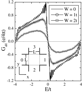
Figure 1: Spin-Hall conductance $G_{sH}$ for some disorder strengths as a function of electron Fermi energy $E$. Here, the sample size $L=40$ and the spin-orbit coupling $V_{\mbox{\tiny SO}}=0.5t$. Inset is a schematic view of the four-terminal junction.

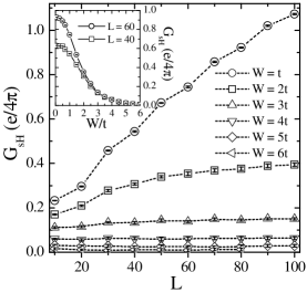
Figure 2: Spin-Hall conductance as a function of sample size $L$ for different disorder strengths at $E=-2t$ and $V_{\mbox{\tiny SO}}=0.5t$. Error bars due to statistical fluctuations, being smaller than the symbol size, are drawn inside the open symbols. Inset: spin-Hall conductance as a function of disorder strength for $L=40$ and $60$.

In order to determine the behavior of the spin-Hall effect in large systems, we calculate the SHC as a function of the sample size from $L=10$ up to $100$ for different strengths of disorder, as shown in Fig. 2. For weak disorder $W\lesssim 3t$, the SHC first increases with increasing sample size, and then tends to saturate. In particular, for $W\lesssim t$, we see that the SHC can be several times greater than the universal value $e/8\pi$, when the system becomes large. For a stronger disorder $3t\lesssim W\lesssim 5t$, the SHC is roughly independent of the sample size, and extrapolates to a finite value in the large-size limit. Therefore, it is evident that the SHC will not vanish in large systems in the presence of moderately strong disorder $W\lesssim 5t$. With further increase of $W$, the SHC becomes vanishingly small at $W\gtrsim 6t$, as seen more clearly from the inset of Fig. 2, indicating that very strong disorder scattering would eventually destroy the spin-Hall effect.

We further examine the dependence of the SHC on the strength of the SO coupling. As shown in Fig. 3, overall, the SHC increases with increasing $V_{\mbox{\tiny SO}}$ in the range $0\leq V_{\mbox{\tiny SO}}\leq t$. For $W=0$ or weak disorder, the SHC displays an interesting oscillation effect with a period much greater than the average level spacing. According to Eq. (2), the oscillation of the SHC is a manifestation of the oscillation of the sideway spin-resolved transmission coefficients. For a two-terminal junction with the SO coupling, similar oscillation with finite sample size has previously been observed for the spin-resolved transmission coefficients Echo , where the oscillation period was discussed to be the spin precession length $L_{sp}$. If we apply the same condition $L=nL_{sp}$ with $n$ an integer and notice $L_{sp}\simeq\pi t/V_{\mbox{\tiny SO}}$, Echo we can obtain for the equivalent period in the SO coupling $\delta V_{\mbox{\tiny SO}}\simeq\pi t/L$. For the parameters used in Fig. 3, $\delta V_{\mbox{\tiny SO}}\simeq 0.08t$, which is very close to the period as seen in the figure. This indicates that the oscillation of the SHC is due to a spin precessional effect in finite-size systems. Experimentally, $V_{\mbox{\tiny SO}}$ can be varied over a wide range by tuning a gate voltage r1 ; h3 , and so this oscillation effect may possibly be observed directly.

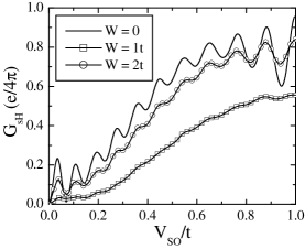
Figure 3: Spin-Hall conductance as a function of spin-orbit coupling strength for some disorder strengths. Here, the sample size $L=40$ and the electron Fermi energy $E=-2t$.

Electron delocalization is a crucial issue for understanding electron transport properties in the 2DES, and has already been studied experimentally by use of magnetoresistance measurements h3 . For this reason, we investigate numerically whether the Rashba SO coupling can induce a universal electron delocalization in the presence of disorder. According to the well-established transfer matrix approach, h4 ; lisheng we calculate the electron localization length $\xi$ on a bar of essentially infinite length ($5\times 10^{5}$) and finite width $L$. In Fig. 4a, the normalized localization length $\xi/L$ is plotted as a function of disorder strength for $V_{\mbox{\tiny SO}}=0.5t$ and $L=8$, 16, 32 and 64. At weak disorder, $\xi/L$ increases with $L$, indicating that the localization length $\xi$ will diverge as $L\rightarrow\infty$, corresponding to an electron delocalized metallic phase. With the increase of $W$, $\xi/L$ goes down and all the curves cross at a point (fixed point) $W=W_{c}\simeq 6.3t$, where $\xi/L$ becomes independent of bar width $L$. For $W>W_{c}$, $\xi/L$ decreases with $L$, indicating that $\xi$ will converge to finite values as $L\rightarrow\infty$, corresponding to an electron localized insulator phase. Thus the fixed point $W=W_{c}$ is the critical disorder strength for the metal-insulator transition. Our result is consistent with the earlier calculation by Ando h1 , where a metallic phase was established at the band center $E=0$ for a strong Rashba SO coupling.

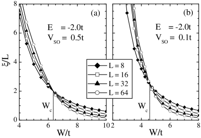
Figure 4: Normalized localization length as a function of disorder strength calculated on long bars of length $5\times 10^{5}$ and widths $L=8$, 16, 32 and 64.

Here, we also study weak SO coupling. In Fig. 4b, we plot the result for a SO coupling strength much smaller than the electron hopping integral, i.e., $V_{\mbox{\tiny SO}}=0.1t$, and similar phase transition is also revealed at $W_{c}\simeq 4.6t$. In general, we have performed calculations in the whole range from strong to weak SO coupling (details will be presented elsewhere), and found that electron delocalization occurs for any nonzero SO coupling strength as the magnitude of the disorder varies. Our result is in agreement with the perturbative calculation of weak localization. WeakLoc As $V_{\mbox{\tiny SO}}$ reduces, the critical $W_{c}$ decreases, and the size-independent critical $\xi/L$ increases (so does the critical longitudinal conductance $G_{xx}$ h4 ; lisheng ). In the limit $V_{\mbox{\tiny SO}}\rightarrow 0$, we have $W_{c}\rightarrow 0$ and all electron states become localized, recovering the known regime of the two-dimensional Anderson model for electron localization h4 . The fact that the critical $\xi/L$ changes with $V_{\mbox{\tiny SO}}$ indicates that the SO coupled 2DES belongs to the universality class of two-parameter scaling NewDNS . Comparing $W_{c}=6.3t$ calculated in Fig. 4a for $V_{\mbox{\tiny SO}}=0.5t$ and $E=-2t$ with the SHC shown in Fig. 2 for the same parameters, we see that nonvanishing spin-Hall effect exists mainly in the metallic regime.

Our numerical study addresses the spin-Hall effect in a finite-size junction system with leads. A comparison between the spin-Hall effect and the quantum Hall effect (QHE) can shed some light on the nonuniversal SHC obtained. For a QHE system, delocalized states exist at the centers of the discrete Landau levels, which are separated by mobility gaps consisting of localized states. In the unit of conductance quantum $e^{2}/h$, the Hall conductance is known to be a sum of the topological Chern numbers of all the occupied delocalized states below the Fermi energy dns1997 . If the Fermi energy lies in a mobility gap, the Hall conductance is well quantized to an integer. If the Fermi energy is at a critical point, where a delocalized state exists, the Hall conductance intrinsically fluctuates between two integers. Similarly, the SHC is also related to corresponding topological numbers of the occupied delocalized states. However, in the present spin-Hall systems, the delocalized states constitute a continuous spectrum without mobility gaps (or energy gaps h1 ). Due to the lack of a mobility gap around the Fermi energy, the SHC can fluctuate and does not show quantized plateaus. As a matter of fact, the universal value $e/8\pi$ predicted for clean bulk systems t2 is 0.5 instead of an integer in the unit of spin conductance quantum $e/4\pi$ (here the electron charge $e$ in the conductance quantum $e^{2}/h$ needs be replaced with electron spin $\hbar/2$). For the above reason, one could not expect that the SHC will not change to different values under different boundary conditions. In the present junction system, the open boundary, i.e., the connection of the finite-size sample with the much larger semi-infinite leads is quite different from the essentially close boundary used in previous calculations t2 ; t6 ; tt7 ; t7 ; t9 ; t10 ; t12 ; t14 ; t15 , which is likely the cause for the SHC to be possibly greater or smaller than $e/8\pi$ depending on the electron Fermi energy, the disorder strength and the magnitude of the SO coupling. Notably, the analytical calculation t14 also indicates that the contacts between a sample and leads could enhance the generation of spin currents. Our calculations provide an important evidence that the proposed intrinsic spin-Hall effect t1 ; t2 may be realized experimentally in junction systems in the presence of disorder.

Note added: After initial submission of this paper, we became aware of a couple preprints by Nikolić, Zârbo and Souma and by Hankiewicz $et$ $al.$ nikoli , where similar LB formula calculations were carried out. Despite different parameter values used, their results of nonuniversal SHC robust against disorder scattering are consistent with ours.

Acknowledgment: The authors would like to thank A. H. MacDonald, Q. Niu and J. Sinova for stimulating discussions. This work is supported by ACS-PRF 41752-AC10, Research Corporation Award CC5643, the NSF grant/DMR-0307170 (DNS), and also by a grant from the Robert A. Welch Foundation (CST). DNS wishes to thank the Aspen Center for Physics and Kavli Institute for Theoretical Physics for hospitality and support (through PHY99-07949 from KITP), where part of this work was done.

References

- (1) S. A. Wolf , Science 294, 1488 (2001).
- (2) D. D. Awschalom, D. Loss, and N. Samarth, Semiconductor Spintronics and Quantum Computation (Springer-Verlag, Berlin, 2002).
- (3) R. Fiederling , Nature 402, 787 (1999); G. Schmidt, and L. W. Molenkamp, Semi. Si. Tech. 17, 310 (2002).
- (4) H. Ohno, Science 281, 951 (1998); 4313 (1998).
- (5) B. T. Jonker, Proc. IEEE 91, 727 (2003).
- (6) S. Murakami, N. Nagaosa, and S. C. Zhang, Science 301, 1348 (2003).
- (7) J. Sinova , Phys. Rev. Lett. 92, 126603 (2004).
- (8) T. P. Pareek, Phys. Rev. Lett. 92, 076601 (2004).
- (9) J. Hu, B. A. Bernevig and C.Wu, cond-mat/0310093; S. -Q. Shen, Phys. Rev. B 70, R081311 (2004).
- (10) A. A. Burkov, A. S. Nunez and A. H. MacDonald, cond-mat/0311328.
- (11) J. Schliemann and D. Loss, Phys. Rev. B 69, 165315 (2004).
- (12) E. I. Rashba, cond-mat/0311110; cond-mat/0404723.
- (13) O. V. Dimitrova, cond-mat/0405339.
- (14) J. I. Inoue, G. E. W. Bauer, and L. W. Molenkamp, cond-mat/0402442.
- (15) E. G. Mishchenko, A. V. Shytov, and B. I. Halperin, cond-mat/040673.
- (16) K. Nomura , cond-mat/0407279.
- (17) S. Murakami, N. Nagaosa, and S. C. Zhang, cond-mat/0406001.
- (18) T. Ando, Phys. Rev. B 40, 5325 (1989).
- (19) T. P. Pareek and P. Bruno, Phys. Rev. B 65, 241305 (2002).
- (20) M. Büttiker, Phys. Rev. Lett. 57, 1761(1986).
- (21) R. Landauer, Philos. Mag. 21, 863 (1970).
- (22) S. Datta, Electronic Transport in Mesoscopic Systems (Cambridge University Press, Cambridge, 1995).
- (23) Y. Meir and N. S. Wingreen, Phys. Rev. Lett. 68, 2512(1992).
- (24) F. G. Moliner and V. R. Velasco, Phys. Rep. 200, 83 (1991); J. Appelbaum and D. Hamann, Phys. Rev. B 6, 2166 (1972); K. Wood and J. B. Pendry, Phys. Rev. Lett. 31, 1400 (1973); J. Zhang, Q. W. Shi, and J. Yang, J. Chem. Phys. 120, 7733(2004).
- (25) D. N. Sheng and Z. Y. Weng, Phys. Rev. Lett. 78, 318(1997).
- (26) J. Nitta, T. Akazaki, H. Takayanagi, and T. Enoki, Phys. Rev. Lett. 78, 1335 (2003).
- (27) D. M. Zumbühl , Phys. Rev. Lett. 89, 276803 (2002); J. B. Miller , Phys. Rev. Lett. 90, 76807(2003).
- (28) A. MacKinnon and B. Kramer, Phys. Rev. Lett. 47, 1546 (1981); Z. Phys. B 53, 1 (1983).
- (29) L. Sheng, D. Y. Xing, D. N. Sheng and C. S. Ting, Phys. Rev. B 56, R7053 (1997); Phys. Rev. Lett. 79, 1710 (1997).
- (30) M. A. Skvortsov, JETP Letters, 67, 133 (1998).
- (31) D. N. Sheng and Z. Y. Weng, Phys. Rev. Lett. 80, 580 (1998).
- (32) B. K. Nikolić, L. P. Zârbo and S. Souma, cond-mat/0408693 (2004); E. M. Hankiewicz, L. W. Molenkamp, T. Jungwirth, and J. Sinova, cond-mat/0409334 (2004).