Self-avoiding walks and polygons on the triangular lattice

Abstract

We use new algorithms, based on the finite lattice method of series expansion, to extend the enumeration of self-avoiding walks and polygons on the triangular lattice to length 40 and 60, respectively. For self-avoiding walks to length 40 we also calculate series for the metric properties of mean-square end-to-end distance, mean-square radius of gyration and the mean-square distance of a monomer from the end points. For self-avoiding polygons to length 58 we calculate series for the mean-square radius of gyration and the first 10 moments of the area. Analysis of the series yields accurate estimates for the connective constant of triangular self-avoiding walks, $\mu=4.150797226(26)$, and confirms to a high degree of accuracy several theoretical predictions for universal critical exponents and amplitude combinations.

1 Introduction

Self-avoiding walks (SAWs) and polygons (SAPs) on regular lattices are combinatorial problems of tremendous inherent interest as well as serving as simple models of polymers and vesicles [25, 15, 16]. They are fundamental problems in lattice statistical mechanics. An $n$-step self-avoiding walk $\bm{\omega}$ is a sequence of distinct vertices $\omega_{0},\omega_{1},\ldots,\omega_{n}$ such that each vertex is a nearest neighbour of it predecessor. SAWs are considered distinct up to translations of the starting point $\omega_{0}$. We shall use the symbol $\bm{\Omega}_{n}$ to mean the set of all SAWs of length $n$. A self-avoiding polygon of length $n$ is a $n-1$-step SAW such that $\omega_{0}$ and $\omega_{n-1}$ are nearest neighbours and a closed loop can be formed by inserting a single additional step. One is interested in the number of SAWs and SAPs of length $n$, various metric properties such as the radius of gyration, and for SAPs one can also ask about the area enclosed by the polygon. In this paper we study the following properties:

• the number of $n$-step self-avoiding walks $c_{n}$;

• the number of $n$-step self-avoiding polygons $p_{n}$;

• the mean-square end-to-end distance of $n$-step SAWs $\langle R^{2}_{e}\rangle_{n}$;

• the mean-square radius of gyration of $n$-step SAWs $\langle R^{2}_{g}\rangle_{n}$;

• the mean-square distance of a monomer from the end points of $n$-step SAWs $\langle R^{2}_{m}\rangle_{n}$;

• the mean-square radius of gyration of $n$-step SAPs $\langle R^{2}\rangle_{n}$; and

• the $k^{\rm th}$ moment of the area of $n$-step SAPs $\langle a^{k}\rangle_{n}$.

The metric properties for SAWs are defined by,

$$\langle R^{2}_{e}\rangle_{n}=\frac{1}{c_{n}}\sum_{\bm{\Omega}_{n}}(\omega_{0}-\omega_{n})^{2},$$

$$\langle R^{2}_{g}\rangle_{n}=\frac{1}{c_{n}}\sum_{\bm{\Omega}_{n}}\left[\frac{1}{2(n+1)^{2}}\sum_{i,j=0}^{n}(\omega_{i}-\omega_{j})^{2}\right],$$

$$\langle R^{2}_{m}\rangle_{n}=\frac{1}{c_{n}}\sum_{\bm{\Omega}_{n}}\left[\frac{1}{2(n+1)}\sum_{i=0}^{n}\left[(\omega_{0}-\omega_{j})^{2}+(\omega_{n}-\omega_{j})^{2}\right]\right],$$

with a similar definition for the radius of gyration of SAPs.

It is generally believed that the quantities listed above has the asymptotic forms as $n\to\infty$:

$$c_{n}=A\mu^{n}n^{\gamma-1}[1+o(1)],$$ (1.1a)

$$p_{n}=B\mu^{n}n^{\alpha-3}[1+o(1)],$$ (1.1b)

$$\langle R^{2}_{e}\rangle_{n}=Cn^{2\nu}[1+o(1)],$$ (1.1c)

$$\langle R^{2}_{g}\rangle_{n}=Dn^{2\nu}[1+o(1)],$$ (1.1d)

$$\langle R^{2}_{m}\rangle_{n}=En^{2\nu}[1+o(1)],$$ (1.1e)

$$\langle R^{2}\rangle_{n}=Fn^{2\nu}[1+o(1)],$$ (1.1f)

$$\langle a^{k}\rangle_{n}=G^{(k)}n^{2\nu k}[1+o(1)].$$ (1.1g)

The critical exponents are believed to be universal in that they only depend on the dimension of the underlying lattice. The connective constant $\mu$ and the critical amplitudes $A$–$G^{(k)}$ vary from lattice to lattice. In two dimensions the critical exponents $\gamma=43/32$, $\alpha=1/2$ and $\nu=3/4$ have been predicted exactly, though non-rigorously, using Coulomb-gas arguments [26, 27].

While the amplitudes are non-universal, there are many universal amplitude combinations. Any ratio of the metric SAW amplitudes, e.g. $D/C$ and $E/C$, is expected to be universal [6]. Of particular interest is the linear combination [6, 2] (which we shall call the CSCPS relation)

$$H\;\equiv\;\left(2+\frac{y_{t}}{y_{h}}\right)\frac{D}{C}\,-\,2\frac{E}{C}\,+\,\frac{1}{2},$$ (1.1b)

where $y_{t}=1/\nu$ and $y_{h}=1+\gamma/(2\nu)$. In two dimensions Cardy and Saleur [6] (as corrected by Caracciolo, Pelissetto and Sokal [2]) have predicted, using conformal field theory, that $H=0$. This conclusion has been confirmed by previous high-precision Monte Carlo work [2] as well as by series extrapolations [14].

Privman and Redner [29] proved that the combination $BC/\sigma a_{0}$ is universal, Cardy and Guttmann [4] proved that $BF=\frac{5}{32\pi^{2}}\sigma a_{0}$, and Cardy and Mussardo [5] proved that $C/F$ is universal and gave the first theoretical estimate of the value $C/F\approx 13.70$. $\sigma$ is an integer constant such that $p_{n}$ is non-zero when $n$ is divisible by $\sigma$. So $\sigma=1$ for the triangular lattice and 2 for the square and honeycomb lattices. $a_{0}$ is the area per lattice site and $a_{0}=1$ for the square lattice, $a_{0}=3\sqrt{3}/4$ for the honeycomb lattice, and $a_{0}=\sqrt{3}/2$ for the triangular lattice.

Richard, Guttmann and Jensen [30] conjectured the exact form of the critical scaling function for self-avoiding polygons and consequently showed that the amplitude combinations $G^{(k)}B^{k-1}$ are universal and predicted their exact values. The exact value for $G^{(1)}=\frac{1}{4\pi}$ had previously been predicted by Cardy [3]. The validity of this conjecture was recently confirmed numerically to a high degree of accuracy using exact enumeration data for SAPs on the square, honeycomb, and triangular lattices [31].

The asymptotic form (1.1a) only explicitly gives the leading contribution. In general one would expect corrections to scaling so, e.g,

$$c_{n}=A\mu^{n}n^{\gamma-1}\left[1+\frac{a_{1}}{n}+\frac{a_{2}}{n^{2}}+\ldots+\frac{b_{0}}{n^{\Delta_{1}}}+\frac{b_{1}}{n^{\Delta_{1}+1}}+\frac{b_{2}}{n^{\Delta_{1}+2}}+\ldots\right]$$ (1.1c)

In addition to “analytic” corrections to scaling of the form $a_{k}/n^{k}$, there are “non-analytic” corrections to scaling of the form $b_{k}/n^{\Delta_{1}+k}$, where the correction-to-scaling exponent $\Delta_{1}$ isn’t an integer. In fact one would expect a whole sequence of correction-to-scaling exponents $\Delta_{1}<\Delta_{2}\ldots$, which are both universal and also independent of the observable, that is, the same for $c_{n}$, $p_{n}$, and so on. In a recent paper [1] we study the amplitudes and the correction-to-scaling exponents for two-dimensional SAWs, using a combination of series-extrapolation and Monte Carlo methods. We enumerated all self-avoiding walks up to 59 steps on the square lattice, and up to 40 steps on the triangular lattice, measuring the metric properties mentioned above, and then carried out a detailed and careful analysis of the data in order to accurately estimate the amplitudes and correction-to-scaling exponent. The analysis provides firm numerical evidence that $\Delta_{1}=3/2$ as predicted by Nienhuis [26, 27].

In this paper we give a detailed account of the algorithm used to calculate the triangular lattice series analysed in [1, 31], perform some further analysis of the series and confirm to great accuracy the predicted exact values of the critical exponents, then we briefly summarise the results of the analysis from [1, 31] and finally study other amplitude combinations.

2 Enumeration of self-avoiding walks and polygons

The use of transfer-matrix methods for the enumeration of lattice objects has its origin in the pioneering work of Enting [10] who enumerated square lattice self-avoiding polygons using the finite lattice method. The basic idea of the finite lattice method is to calculate partial generating functions for various properties of a given model on finite pieces, say $W\times L$ rectangles of the square lattice, and then reconstruct a series expansion for the infinite lattice limit by combining the results from the finite pieces. The generating function for any finite piece is calculated using transfer matrix (TM) techniques. The algorithm we use to enumerate SAWs and SAPs on the triangular lattice builds on this approach and more specifically our algorithm is based in large part on the one devised by Enting and Guttmann [11] for the enumeration of SAPs on the triangular lattice with the generalisation to SAWs following the work of Conway, Enting and Guttmann [7] and using further recent enhancements and parallelisation as described in [19, 20].

2.1 Basic transfer matrix algorithm

In this section we give a detailed description of the SAW algorithm and then briefly outline the changes required to enumerate SAPs.

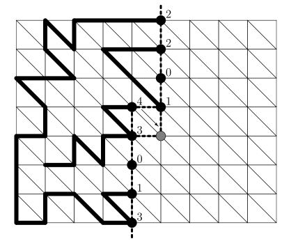
Figure 1: A snapshot of the boundary line (dashed line) during the transfer matrix calculation on the triangular lattice. SAWs are enumerated by successive moves of the kink in the boundary line so that one vertex (shaded) at a time is added to the rectangle. To the left of the boundary line we have drawn an example of a partially completed SAW.

We implement the triangular lattice as a square lattice with additional edges connecting the top-left and bottom-right vertices of each unit cell (see fig 1). We use $W\times L$ rectangles as our finite lattices. The most efficient implementation of the TM algorithm generally involves bisecting the finite lattice with a boundary (this is just a line in the case of rectangles) and moving the boundary in such a way as to build up the lattice cell by cell. The sum over all contributing graphs is calculated as the boundary is moved through the lattice. Due to the symmetry of the triangular lattice we need only consider rectangles with $L\geq W$. SAWs in a given rectangle are enumerated by moving the intersection so as to add one vertex at a time, as shown in figure 1. In most cases it is most efficient to let the boundary line cut through the edges of the lattice. However, on the triangular lattice it is more efficient to let the boundary line cut through the vertices [11]. Essentially this variation leads to only half as many intersected vertices (as opposed to edges) along the boundary line. For each configuration of occupied or empty vertices along the intersection we maintain a generating function for partial walks cutting the intersection in that particular pattern. If we draw a SAW and then cut it by a line we observe that the partial SAW to the left of this line consists of a number of loops connecting two vertices (we shall refer to these vertices as loop-ends) in the intersection, and pieces which are connected to only one vertex (we call these free ends). The other end of the free piece is an end point of the SAW so there are at most two free ends. In addition it is possible that the SAW touches a vertex (that is the SAW comes in along one edge and exits along another edge both without crossing the boundary line). All these cases are illustrated in figure 1. In applying the transfer matrix technique to the enumeration of SAWs we regard them as sets of edges on the finite lattice with the properties:

• A weight $u$ is associated with an occupied edge.

• All vertices are of degree 0, 1 or 2.

• There are at most two vertices of degree 1 and the final graph has exactly two vertices of degree 1 (the end points of the SAW).

• Apart from isolated sites, the final graph has a single connected component.

• Each graph must span the rectangle from left to right and from bottom to top.

We are not allowed to form closed loops, so two loop-ends can only be joined if they belong to different loops. To exclude loops which close on themselves we need to label the occupied vertices in such a way that we can easily determine whether or not two loop-ends belong to the same loop. The most obvious choice would be to give each loop a unique label. However, on two-dimensional lattices there is a more compact scheme relying on the fact that two loops can never intertwine. Each end of a loop is assigned one of two labels depending on whether it is the lower end or the upper end of a loop. Each configuration along the boundary line can thus be represented by a set of states $\{\sigma_{i}\}$, where

$$\sigma_{i}=\left\{\begin{array}[]{rl}0&\;\;\;\mbox{empty vertex},\\ 1&\;\;\;\mbox{vertex is a lower loop-end},\\ 2&\;\;\;\mbox{vertex is an upper loop-end},\\ 3&\;\;\;\mbox{touched (degree 2) vertex},\\ 4&\;\;\;\mbox{vertex is a free end}.\\ \end{array}\right.$$ (1.1a)

If we read from the bottom to the top, the configuration along the intersection of the partial SAW in figure 1 is $\{310341022\}$.

2.1.1 Updating rules

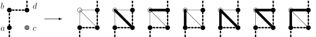
Figure 2: The seven possible outputs from a single iteration of the TM algorithm. Depending on the states of the three vertices $a$, $b$, and $d$ in the input some of the outputs cannot occur.

In figure2 we have illustrated what can happen locally as the boundary line is moved. Before the move, the boundary line intersects the vertices $a$, $b$ and $d$ and after the move the vertices $a$, $c$ and $d$ are intersected by the boundary line. We shall refer to the boundary line configuration prior to a move as the ‘source’ and after the move as the ‘target’. In a basic iteration step we can insert bonds along the edges emanating from vertex $b$. Since vertex $b$ can’t have degree greater than 2 we can at most insert two new bonds. However, depending on the states of vertices $a$ and $d$ in the source, some of the edge configuration in figure 2 may be forbidden. The updating of the partial generating function depends most crucially on the state of vertex $b$ and to a somewhat lesser extent on the states of the vertices $a$ and $d$. The basic limitation on the allowed outputs are that conditions (2)–(4) must be enforced. In the following we shall briefly describe how the updating rules are derived.

State of vertex $\bm{b}$ is 0. Since vertex $b$ is empty all the outputs in figure 2 are possible. In the first output we insert no bonds. This is always allowed and no changes are made to the configuration.

In the next three outputs we insert a single bond. This makes vertex $b$ of degree one and is thus only allowed if there is at most one free end in the source. There are further restrictions on the insertion of a bond to vertices $a$ or $d$. Firstly if a vertex is touched (in state 3) we cannot insert a bond since this would result in a vertex of degree 3. Secondly if the vertex is a free end (in state 4) we join two free ends. This leads to the formation of a completed sub-graph and is only permitted if the resulting graph is a valid SAW. So the configuration cannot contain other pieces of a SAW and the only permissible states of other vertices in the intersection are 0 and 3. If a valid SAW is created we multiply the source generating function by $u$ (representing the new bond) before adding it to the total for the SAW generating function.

In the last three outputs we insert a partial loop. Again there are restrictions on the insertion of bonds to vertices $a$ and $d$. As before we cannot insert a bond to a vertex in state 3. Otherwise the first two outputs are always allowed. The last output is a little more complicated. If both vertices $a$ and $d$ are in state 4 we join two free ends and as before we check if the result is a valid SAW and if so add this partial generating function the SAW generating function (this time we multiply the source generating function by $u^{2}$). If vertex $a$ is in state 1 and vertex $d$ in state 2 we cannot join the two vertices since this would result in a closed loop.

After the insertion of new bonds we have to assign a state to vertex $c$ and quite possibly change the states of vertices $a$ and $d$ (and perhaps the states of some other vertices in the target configuration). The state of vertex $c$ will be 0 (no bond), 1 (lower loop-end), 2 (upper loop-end) or 4 (free end). Next we consider what happens to vertices $a$ and $d$. When these vertices are empty in the source they can take the values just listed above in the target. If they are occupied in the source they either retain their state in the target (no bonds inserted) or change to state 3 (a bond is inserted). In the latter case we may have to change the state of other vertices in the target. If we insert a free end and it joins a lower (upper) loop-end we must change the matching upper (lower) loop-end to a free end. Otherwise we may join two lower (upper) loop-ends and then we must change the matching upper (lower) loop-end of the inner most loop to the lower (upper) loop-end of the new joined loop.

State of vertex $\bm{b}$ is 1. A lower end of a loop enters vertex $b$. If we insert no further bonds a new degree 1 vertex is created. As above this is only allowed provided the source has at most one free end. The matching upper loop-end becomes a free end. Otherwise the lower end has to be continued by inserting a single bond (partial loops cannot be inserted since this would make vertex $b$ of degree 3) either to vertex $c$ which becomes a state 1 vertex; to vertex $a$ if not in state 3 or state 2 (closed loop would be formed); or to vertex $d$ if not in state 3. Again we have to change the states of vertices $a$ and $d$ when a bond is inserted on these vertices. If the source state of the vertices was 0 the target state becomes 1, otherwise the target state becomes 3 and as above we may need to change the state of other vertices as well.

State of vertex $\bm{b}$ is 2. An upper end of a loop enters vertex $b$. If we terminate the loop-end a new degree 1 vertex is created. Again this is only allowed provided the source has at most one free end. The matching lower end of the loop becomes a free end. The upper end can always be continued to vertex $c$; to vertex $d$ if it is not in state 3; and to vertex $a$ provided it is not in state 3 or 1 (this would result in a closed loop). The state of the target vertices are changed as described above.

State of vertex $\bm{b}$ is 3. This is the simplest situation. Vertex $b$ is of degree 2 so no bonds can be inserted and only the output with all empty edges is allowed. The state of vertex $c$ is 0 and the states of all other vertices are unchanged.

State of vertex $\bm{b}$ is 4. A free end is entering vertex $b$. If we insert no further bonds a partial walk is terminated at the vertex. This is only allowed if the resulting graph is a valid SAW and the source generating function is added to the SAW generating function. The free end can always be continued to vertex $c$ and to vertices $a$ and $d$ if they are not in state 3. As before, if we join two free ends we check if it is a valid SAW and then add the partial generating function (multiplied by $u$) to the SAW generating function. Otherwise the target configuration is updated as described previously.

SAP updating rules.

The updating rules used when enumerating SAPs are essentially just a subset of the SAW rules. Obviously there are no degree 1 vertices in the SAP case so we can’t insert a single bond if vertex $b$ is empty. Likewise if vertex $b$ is occupied we must continue the loop-end. Completed SAPs are formed by closing a loop (if there are no other loop-ends in the source). This happens when the local source configuration $\{abd\}$ is $\{120\}$ and we insert a bond from $b$ to $a$, $\{102\}$ and we insert a partial loop from $a$ through $b$ to $d$, or $\{012\}$ and we insert a bond from $b$ to $d$.

2.1.2 Pruning

The use of pruning to obtain more efficient TM algorithms was used for square lattice SAPs in [21]. Numerically it was found that the computational complexity was close to $2^{n/4}$, much better than the $3^{n/4}$ of the original approach. We have used similar techniques for the enumerations carried out for this paper. Pruning allows us to discard most of the possible configurations for large $W$ because they only contribute at lengths greater than $N_{\rm max}$, where $N_{\rm max}$ is the maximal length to which we choose to carry out our calculations. The value of $N_{\rm max}$ is limited by the available computational resources, be they CPU time or physical memory. Briefly pruning works as follows. Firstly, for each configuration we keep track of the current minimum number of steps $N_{\rm cur}$ already inserted to the left of the boundary line in order to build up that particular configuration. Secondly, we calculate the minimum number of additional steps $N_{\rm add}$ required to produce a valid SAP or SAW. There are three contributions, namely the number of steps required to connect the loops and free ends, the number of steps needed (if any) to ensure that the SAW touches both the lower and upper border, and finally the number of steps needed (if any) to extend at least $W$ edges in the length-wise direction (remember we only need rectangles with $L\geq W$). If the sum $N_{\rm cur}+N_{\rm add}>N_{\rm max}$ we can discard the partial generating function for that configuration, and of course the configuration itself, because it won’t make a contribution to the count up to the lengths we are trying to obtain.

There are no principal differences between pruning SAWs and SAPs though the detailed implementation is more complicated for the SAW case. We found it necessary to explicitly write subroutines to handle the three distinct cases where the TM configuration contains zero, one and two free ends, respectively. But in all cases we essentially have to go through all the possible ways of completing a SAW in order to find the minimum number of steps required. This is a fairly straightforward task though quite time consuming.

2.1.3 Computational complexity

The time $T(n)$ required to obtain the number of polygons or walks of length $n$ grows exponentially with $n$, $T(n)\propto\lambda^{n}$. For the algorithm without pruning the complexity can be calculated exactly. Time (and memory) requirements are basically proportional to a polynomial (in $n$) times the maximal number of configurations, $N_{\rm Conf}$, generated during a calculation. When the boundary line is straight we can find the exact number of configurations. First look at the situation for SAPs when there are no free ends. The configurations correspond to 2-coloured Motzkin paths [9], since we can map empty and touched vertices to the two colours of horizontal steps, vertices in the lower state to a north-east step, and vertices in the upper state to a south-east step. The number of such paths $M_{n}$ with $n$ steps is easily derived from the generating function [9]

$$M(x)=\sum_{n}M_{n}x^{n}=[1-2x-(1-4x)^{1/2}]/2x^{2},$$ (1.1b)

which means that $M_{n}\sim 4^{n}$ as $n\to\infty$. Note that $M_{n}$ slightly over counts $N_{\rm Conf}$ since configurations without a loop aren’t permitted, but since there are only $2^{W}$ of these there is no change in the asymptotic growth. When the boundary line has a kink (such as in figure 1) $N_{\rm Conf}$ is no longer given exactly by $M_{W}-2^{W}$. However, it is obvious that $N_{\rm S}(W+1)\leq N_{\rm Conf}\leq N_{\rm S}(W)$ so we see that asymptotically $N_{\rm Conf}$ grows like $4^{W}$. Since a calculation using rectangles of widths $\leq W$ yields the number of SAPs up to $n=2W+1$ it follows that the complexity of the algorithm is $T(n)\propto\lambda^{n}$ with $\lambda=2$.

The number of transfer matrix configurations in the unpruned SAW algorithm is simply obtained by inserting 0, 1 or 2 free ends into a 2-coloured Motzkin path and eliminating the paths corresponding to a configurations with only empty or touched vertices. In this case a calculation using rectangles of widths $\leq W$ yields the number of SAWs up to $n=W$ it follows that the complexity of the algorithm is $T(n)\propto\lambda^{n}$ with $\lambda=4$.

The pruned algorithm is much too difficult to analyse exactly. So all we can give is a numerical estimate of the growth in the number of configurations with $n$. That is obtained by just running the algorithm and measuring the maximal number of configurations generated for different values of $n$. From the actual numbers it appears that for the SAP case increasing $n$ by 2 increases the number of configurations by slightly less than a factor of 2. This would mean that for the pruned SAP algorithm $\lambda_{p}\approx\sqrt{2}$. In the SAW case it appears that increasing $n$ by 4 increases the number of configuration by a factor close to 5. So for the pruned SAW algorithm $\lambda_{p}\approx\sqrt[4]{5}=1.495\ldots$. So once again pruning results in much more efficient algorithms.

2.1.4 Parallelisation

The transfer-matrix algorithms used in the calculations of the finite lattice contributions are eminently suited for parallel computation. The bulk of the calculations for this paper were performed on the facilities of the Australian Partnership for Advanced Computing (APAC). The APAC facility is an HP Alpha server cluster with 125 ES45’s each with four 1 Ghz chips for a total of 500 processors in the compute partition. Each server node has at least 4 Gb of memory. Nodes are interconnected by a low latency high bandwidth Quadrics network.

The most basic concern in any efficient parallel algorithm is to minimise the communication between processors and ensure that each processor does the same amount of work and uses the same amount of memory. In practice one naturally has to strike some compromise and accept a certain degree of variation across the processors.

One of the main ways of achieving a good parallel algorithm using data decomposition is to try to find an invariant under the operation of the updating rules. That is we seek to find some property of the configurations along the boundary line which does not alter in a single iteration. The algorithm for the enumeration of SAPs and SAWs are quite complicated since not all possible configurations occur due to pruning and an update at a given set of vertices might change the state of a vertex far removed, e.g., when two lower loop-ends are joined we have to relabel one of the associated upper loop-ends as a lower loop-end in the new configuration. However, there is still an invariant since any vertex not directly involved in the update cannot change from being empty to being occupied and vice versa, likewise a touched vertex will remain unchanged. That is only the kink vertices can change their occupation or touched status. This invariant allows us to parallelise the algorithm in such a way that we can do the calculation completely independently on each processor with just two redistributions of the data set each time an extra column is added to the lattice. We have already used this scheme for SAPs [19] and lattice animals [18] and refer the interested reader to these publications for further detail. Our parallelisation scheme is also very similar to that used by Conway and Guttmann [8, 13].

2.2 Metric properties and area-weighted moments

The generalisation of the algorithm required to calculate metric properties and area-weighted moments has been described in detail in [17, 20] in the square lattice case. Only some minor adjustments are needed in order to apply these ideas to metric properties on the triangular lattice (no changes are needed for the area-weighted moments). We have represented the triangular lattice as a square lattice with extra edges along one of the main diagonals in a unit cell. A point $(s,t)$ on the square lattice is the point $(x,y)$ on the triangular lattice where $x=s+\frac{1}{2}t$ and $y=\frac{\sqrt{3}}{2}t$. As shown in [17, 20] calculation of metric properties involves summation over products of the $x$ and $y$ coordinates of the distance vectors. To be explicit we define the radius of gyration according to the vertices of the SAW. Note that the number of vertices is one more than the number of steps. The radius of gyration of $n+1$ points at positions ${\bf r}_{i}$ is

$$(n+1)^{2}\langle R^{2}_{g}\rangle_{n}=\sum_{i>j}({\bf r}_{i}-{\bf r}_{j})^{2}=n\sum_{i}(x_{i}^{2}+y_{i}^{2})-2\sum_{i>j}(x_{i}x_{j}+y_{i}y_{j}).$$ (1.1c)

From the triangular lattice coordinates we see that both $x_{i}x_{j}$ and $y_{i}y_{j}$ carry a factor $\frac{1}{4}$ so in order to ensure that we get integer coefficients we multiply by 4 and the algorithm will thus calculate the coefficients $4(n+1)^{2}c_{n}\langle R^{2}_{g}\rangle_{n}$. In order to do this we maintain five partial generating functions for each possible boundary configuration, namely

• $C(u)$, the number of (partially completed) SAWs.

• $X^{2}_{g}(u)$, the sum over SAWs of the squared components of the distance vectors.

• $X_{g}(u)$, the sum of the $x$-component of the distance vectors.

• $Y_{g}(u)$, the sum of the $y$-component of the distance vectors.

• $XY_{g}(u)$, the sum of the ‘cross’ product of the components of the distance vectors, that is, $\sum_{i>j}(x_{i}x_{j}+y_{i}y_{j})$.

As the boundary line is moved to a new position each target configuration $S$ might be generated from several sources $S^{\prime}$ in the previous boundary position. The partial generating functions are updated as follows, with $(s,t)$ being the coordinates of the newly added vertex on the square lattice:

$$C(u,S) = \sum_{S^{\prime}}u^{n^{\prime}}C(u,S^{\prime}),$$

$$X^{2}_{g}(u,S) = \sum_{S^{\prime}}u^{n^{\prime}}[X^{2}_{g}(u,S^{\prime})+\delta_{g}((2s+t)^{2}+3t^{2})C(u,S^{\prime})],$$

$$X_{g}(u,S) = \sum_{S^{\prime}}u^{n^{\prime}}[X_{g}(u,S)+\delta_{g}(2s+t)C(u,S^{\prime})],$$ (1.1d)

$$Y_{g}(u,S) = \sum_{S^{\prime}}u^{n^{\prime}}[Y_{g}(u,S)+\delta_{g}tC(u,S^{\prime})],$$

$$XY_{g}(u,S) = \sum_{S^{\prime}}u^{n^{\prime}}[XY_{g}(u,S^{\prime})+\delta_{g}(2s+t)X_{g}(u,S^{\prime})+\delta_{g}3tY_{g}(u,S^{\prime})],$$

where $n^{\prime}$ is the number of steps added to the partial SAW. $\delta_{g}=0$ if the new vertex is empty (has degree 0) and $\delta_{g}=1$ if the new vertex is occupied (has degree $>0$).

The updating rules for the other metric properties are generalised similarly.

2.3 Enumeration results

We calculated the number of polygons up to perimeter 60, while the radius of gyration and first 10 area-weighted moments were obtained up to perimeter 58. We calculated the number of SAWs, their mean-square radius of gyration, mean-square end-to-end distance, and the mean-square distance of monomers from the end points. These quantities were obtained for walks up to length 40. The calculations required up to 35Gb of memory using up to 40 processors at a time and in total we used about 15000 CPU hours.

In table 1 we list the number of SAPs and their radius of gyration while in table 2 we list the series for the SAW problem. These series and those for the area-weighted moments are available at www.ms.unimelb.edu.au/~iwan.

Table 1: The number, $p_{n}$, of embeddings of $n$-step polygons on the triangular lattice and their radius of gyration.

$n$	$p_{n}$	$p_{n}n^{2}\langle R^{2}\rangle_{n}$	$n$	$p_{n}$	$p_{n}n^{2}\langle R^{2}\rangle_{n}$
3	2	6	32	2692047018699717	25886228326621869696
4	3	24	33	10352576717684506	110846359749047031012
5	6	102	34	39902392511347329	474213717578995665624
6	15	468	35	154126451419554156	2026979522666735966994
7	42	2172	36	596528356905096920	8657009828812246231296
8	123	9978	37	2313198287784319026	36944420238568755696168
9	380	45816	38	8986249863419780682	157546885404468362432148
10	1212	208686	39	34969337454759091232	671378005865890422968520
11	3966	944766	40	136301962040079085257	2859142640844460643187642
12	13265	4253484	41	532093404471021533628	12168301979788445465498400
13	45144	19046580	42	2080235431107538787148	51756227545091330753357904
14	155955	84891654	43	8144154378525048003270	220011744770726296282498056
15	545690	376756392	44	31927176350778729318192	934740492588407244896782986
16	1930635	1665684774	45	125322778845662829008494	3969252848247139670605665948
17	6897210	7338822888	46	492527188641409773340797	16846468953704095289170900908
18	24852576	32233105398	47	1937931188484341585677962	71466199766730550647612342396
19	90237582	141171369444	48	7633665703654150673637363	303035054640652779166447899354
20	329896569	616694403366	49	30101946001283232799847562	1284380183482800747257353493532
21	1213528736	2687630355198	50	118823919397444557546535851	5441398704214816650431847144246
22	4489041219	11687756315940	51	469508402822449711313115200	23043633507948438933442640818176
23	16690581534	50726031551790	52	1856933773092076293566747007	97548735673726189271333029096494
24	62346895571	219753786787212	53	7351015093472721439659392448	412789876403022674873495520537906
25	233893503330	950403133411176	54	29126027071450640626653986531	1746140617537848477455116275581178
26	880918093866	4103923685277414	55	115500592701344029351721102550	7383765950134760244068261726914950
27	3329949535934	17695343555964594	56	458398255374927436357237021173	31212646862418768098391776139187758
28	12630175810968	76195720234557276	57	1820727406941365079260306390484	131899272021134280524854379727885732
29	48056019569718	327682567452126696	58	7237327695683743010999188700157	557209110506518251250962658184410206
30	183383553173255	1407546930663067986	59	28789332223533619621001538109842
31	701719913717994	6039368800117995984	60	114602547490254934327469368968190

Table 2: The number, $c_{n}$, of embeddings of $n$-step self-avoiding walks on the triangular lattice and their radius of gyration, end-to-end distance and distance of monomers from the end-points.

$n$	$c_{n}$	$\frac{1}{6}c_{n}\langle R^{2}_{e}\rangle_{n}$	$\frac{1}{6}(n+1)^{2}c_{n}\langle R^{2}_{g}\rangle_{n}$	$\frac{1}{6}(n+1)c_{n}\langle R^{2}_{m}\rangle_{n}$
1	6	1	1	1
2	30	12	22	17
3	138	97	282	178
4	618	654	2778	1476
5	2730	3977	23305	10667
6	11946	22624	175194	70359
7	51882	122821	1215740	434708
8	224130	644082	7939156	2557166
9	964134	3288739	49422491	14477823
10	4133166	16440648	295993366	79492861
11	17668938	80783857	1717056604	425633898
12	75355206	391310240	9697408184	2231674940
13	320734686	1872763387	53533130211	11494836257
14	1362791250	8870963422	289769871988	58310378811
15	5781765582	41647686501	1541876281342	291901836462
16	24497330322	194014270964	8081886977224	1444405248178
17	103673967882	897639074623	41801262603145	7074419785415
18	438296739594	4127904278590	213650877117460	34334678700977
19	1851231376374	18879838654237	1080407596025856	165283451747722
20	7812439620678	85930246593928	5411153165106856	789827267540498
21	32944292555934	389382874004291	26865804448156781	3749241090582031
22	138825972053046	1757383045067340	132328831054383256	17689855417349797
23	584633909268402	7902553525660965	647064413113509344	83004601828121876
24	2460608873366142	35417121500633314	3142945284616515512	387503899136724032
25	10350620543447034	158241760294727837	15172247917136636793	1800616777561080887
26	43518414461742966	705008848574456242	72826367061554681960	8330920471773661365
27	182885110185537558	3132749279518281223	347722481262776946768	38390978707292879316
28	768238944740191374	13886614514918779812	1652126117509776447678	176259763248055992656
29	3225816257263972170	61415827107198652263	7813839241496101017943	806446563482615080995
30	13540031558144097474	271046328280157919578	36798230598686798952874	3677867046530479086571
31	56812878384768195282	1193838903060544883615	172603075240086498030932	16722626138383080469074
32	238303459915216614558	5248569464050058190772	806559315077883801952302	75819788411079420147060
33	999260857527692075370	23034474248167644819305	3755672941408238341746325	342850281196290726391195
34	4188901721505679738374	100925879660029490332616	17429779928912903943728776	1546457563237807336247617
35	17555021735786491637790	441524252843364233569911	80636231608943399450377104	6958970268567678359172166
36	73551075748132902085986	1928731794198995523104424	371943975622752362856339418	31245121332848941331142166
37	308084020607224317094182	8413734243045682304542891	1710813401690158618688146075	139991577634597301110308061
38	1290171266649477440877690	36655327788277288494374240	7848181414990001769700643892	625968026891459936611240307
39	5401678666643658402327390	159494618902280757690831541	35911648943670829119431170002	2793684462154188994667777314
40	22610911672575426510653226	693174559672551318610401776	163929038497681452701025717812	12445679176337664122926617782

3 Analysis of the series

The series studied in this paper have coefficients which grow exponentially, with sub-dominant term given by a critical exponent. The generic behaviour is $G(u)=\sum_{n}g_{n}u^{n}\sim(1-u/u_{c})^{-\xi},$ and hence the coefficients of the generating function $g_{n}\sim\mu^{n}n^{\xi-1}$, where $\mu=1/u_{c}$. To obtain the singularity structure of the generating functions we used the numerical method of differential approximants [12]. Our main objective is to obtain accurate estimates for the connective constant $\mu$ and confirm numerically the exact values for the critical exponents $\alpha$, $\gamma$ and $\nu$. Estimates of the critical point and critical exponents were obtained by averaging values obtained from second and third order inhomogeneous differential approximants. The error quoted for these estimates reflects the spread (basically one standard deviation) among the approximants. Note that these error bounds should not be viewed as a measure of the true error as they cannot include possible systematic sources of error.

Once the exact values of the exponents have been confirmed we turn our attention to the “fine structure” of the asymptotic form of the coefficients. In particular we are interested in obtaining accurate estimates for the amplitudes. We do this by fitting the coefficients to the form given by (1.1a)-(1.1g). In this case our main aim is to test the validity of the predictions for the amplitude combinations mentioned in the Introduction.

3.1 Self-avoiding polygons

The expected behaviour of the mean-square radius of gyration (1.1f) and moments of area (1.1g) of SAPs results in the following predictions for the generating functions which we study:

$$\mathcal{R}^{2}_{g}(u) = \sum_{n=3}^{\infty}n^{2}p_{n}\langle R^{2}\rangle_{n}u^{n}=\sum_{n=3}^{\infty}r_{n}u^{n}\propto(1-u\mu)^{-(\alpha+2\nu)},$$ (1.1a)

$$\mathcal{P}^{(k)}(u) = \sum_{n=3}^{\infty}p_{n}\langle a^{k}\rangle_{n}u^{n}=\sum_{n=3}^{\infty}a^{(k)}_{n}u^{n}\propto(1-u\mu)^{2-(\alpha+2k\nu)},$$ (1.1b)

where we have taken into account that the smallest polygon has perimeter 3. Thus we expect these series to have a critical point at $u=u_{c}=1/\mu$, and as stated previously the exponents $\alpha=1/2$ and $\nu=3/4$.

3.1.1 The SAP generating function

In Table 3 we have listed the results from our series analysis of the SAP generating function. It is evident that the estimates for the critical exponent is in complete agreement with the expected value $2-\alpha=3/2$. Based on the estimates we find that $u_{c}=0.24091757(1)$. We found no evidence that the SAP generating function had any other singularities.

Table 3: Estimates for the critical point $u_{c}$ and exponent $2-\alpha$ obtained from second and third order differential approximants to the triangular lattice SAP generating function. $L$ is the order of the inhomogeneous polynomial.

• $L$	Second order DA		Third order DA
  	$u_{c}$	$2-\alpha$	$u_{c}$	$2-\alpha$
  0	0.2409175671(28)	1.5000142(45)	0.2409175706(62)	1.500006(12)
  2	0.2409175709(14)	1.5000076(29)	0.2409175716(30)	1.5000071(58)
  4	0.2409175714(27)	1.5000061(56)	0.2409175699(40)	1.5000078(63)
  6	0.2409175707(29)	1.5000075(58)	0.2409175712(29)	1.5000065(57)
  8	0.2409175724(44)	1.500003(10)	0.2409175662(80)	1.500012(14)
  10	0.2409175717(39)	1.5000051(83)	0.2409175704(22)	1.5000083(41)

If we take the conjecture $\alpha=1/2$ to be true we can obtain a refined estimate for the critical point $u_{c}$. In figure 3 we have plotted estimates for the critical exponent $2-\alpha$ against the number of terms used by the approximant and against estimates for the critical point $u_{c}$, respectively. Each dot represents estimates obtained from a third order inhomogeneous differential approximant. The order of the inhomogeneous polynomial was varied from 0 to 10. As can be seen from the left panel the estimates for the critical exponent clearly include the exact value and appear to settle down as the number of terms increases (though there is a hint of a downwards trend). From the right panel we observe that the estimates cross the line $2-\alpha=3/2$ at a value $u_{c}\simeq 0.2409175745$. Based on this analysis we adopt the value $u_{c}=0.2409175745(15)$ and thus $\mu=4.150797226(26)$ as our final estimates.

Figure 3: Plots of estimates from third order differential approximants for $2-\alpha$ vs., respectively, the number of terms used by the differential approximants (left panel) and $u_{c}$ (right panel).

3.1.2 The radius of gyration

Table 4 lists the results of our series analysis for the SAP radius of gyration generating function. It is evident that the estimates for the critical exponent as obtained from third order differential approximants is in complete agreement with the expected behaviour. The estimates from the second order approximants are generally slightly lower than the expected value. One would generally expect third order differential approximants to be superior since they are better suited to represent complicated functional behaviour. We take this as clear numerical confirmation that $\nu=3/4$.

Table 4: Estimates for the critical point $u_{c}$ and exponent $\alpha+2\nu$ of the SAP radius of gyration generating function.

• $L$	Second order DA		Third order DA
  	$u_{c}$	$\alpha+2\nu$	$u_{c}$	$\alpha+2\nu$
  0	0.24091726(11)	1.99885(27)	0.24091761(30)	2.0001(14)
  2	0.24091727(14)	1.99891(26)	0.24091728(33)	1.99925(64)
  4	0.240917246(95)	1.99881(14)	0.24091713(30)	1.99889(36)
  6	0.240917269(87)	1.99884(14)	0.24091741(19)	1.99935(65)
  8	0.240917239(73)	1.99879(11)	0.24091743(24)	1.99947(78)
  10	0.240917281(96)	1.99888(16)	0.24091737(25)	1.99932(70)

3.1.3 Area-weighted moments

In passing we only briefly mention that our analysis of the generating functions $\mathcal{P}^{(k)}(u)$ for area-weighted SAPs with $k\leq 10$ clearly confirmed the expected values, $2-(\alpha+2k\nu)$, for the critical exponents. Suffice to say that the estimates range from $0.0005(8)$ for $k=1$ to $-13.503(2)$ for for $k=10$.

3.2 Self-avoiding walks

From the expected behaviour (1.1a) of $c_{n}$ and the metric properties of SAWs (1.1c)-(1.1e) we get that the generating functions:

$$\mathcal{C}(u) = \sum_{n=1}^{\infty}c_{n}u^{n}\propto(1-u\mu)^{-\gamma},$$ (1.1c)

$$\mathcal{R}^{2}_{e}(u) = \sum_{n=1}^{\infty}c_{n}\langle R^{2}_{e}\rangle_{n}u^{n}\propto(1-u\mu)^{-(\gamma+2\nu)},$$ (1.1d)

$$\mathcal{R}^{2}_{g}(u) = \sum_{n=1}^{\infty}(n+1)^{2}c_{n}\langle R^{2}_{g}\rangle_{n}u^{n}\propto(1-u\mu)^{-(\gamma+2\nu+2)},$$ (1.1e)

$$\mathcal{R}^{2}_{m}(u) = \sum_{n=1}^{\infty}(n+1)c_{n}\langle R^{2}_{m}\rangle_{n}u^{n}\propto(1-u\mu)^{-(\gamma+2\nu+1)},$$ (1.1f)

where the exponents $\gamma=43/32$ and $\nu=3/4$.

3.2.1 The SAW generating function

In Table 5 we list estimates of the critical point $u_{c}$ and exponent $\gamma$ from the series for the triangular lattice SAW generating function. The estimates were obtained by averaging over those approximants which used at least the first 32 terms of the series. Based on these estimates we conclude that $u_{c}=0.24091753(8)$ and $\gamma=1.34368(6)$. The estimate for $u_{c}$ is compatible with the more accurate estimate $u_{c}=0.2409175745(15)$ obtained above from the analysis of the SAP generating function. The analysis adds further support to the already convincing evidence that the critical exponent $\gamma=43/32=1.34375$ exactly. However, we do observe that both the central estimates for both $u_{c}$ and $\gamma$ are systematically slightly lower than the expected values.

Table 5: Estimates for the critical point $u_{c}$ and exponent $\gamma$ obtained from second and third order differential approximants to the square lattice SAW generating function.

• $L$	Second order DA		Third order DA
  	$u_{c}$	$\gamma$	$u_{c}$	$\gamma$
  0	0.240917491(34)	1.343637(42)	0.240917538(21)	1.343687(23)
  2	0.240917529(37)	1.343677(36)	0.240917537(13)	1.343686(22)
  4	0.240917529(42)	1.343682(47)	0.240917534(30)	1.343682(32)
  6	0.240917524(27)	1.343673(27)	0.240917545(24)	1.343693(25)
  8	0.240917523(28)	1.343668(35)	0.240917543(23)	1.343692(27)
  10	0.240917513(31)	1.343662(29)	0.240917530(22)	1.343679(25)

As for the SAP case we find it useful to plot the behaviour of the estimates for the critical exponent $\gamma$ against both $u_{c}$ and the number of terms used by the differential approximants. This is done in figure 4. Each dot represents estimates obtained from a second order inhomogeneous differential approximant. From the left panel we observe that the estimates of $\gamma$ exhibits a certain upwards drift as the number of terms increases. So the estimates have not yet settled at their limiting value, but there can be no doubt that the predicted exact value of $\gamma$ is fully consistent with the estimates. In the left panel we observe that the $(u_{c},\gamma)$-estimates fall in a narrow range. Note that this range does not include the intersection point between the exact $\gamma$ and the precise $u_{c}$ estimate. This is probably a further reflection of the lack of ‘convergence’ to the true limiting values.

Figure 4: Plots of estimates from second order differential approximants for $\gamma$ vs., respectively, the number of terms used by the differential approximants (left panel) and $u_{c}$ (right panel).

3.2.2 The metric properties

Finally, we turn our attention to the metric properties of SAWs. In Table 6 we have listed the estimates for $u_{c}$ and critical exponents obtained by an analysis of the associated generating functions (1.1d)–(1.1f). The estimates from the radius of gyration $u_{c}=0.2409176(1)$ and $\gamma+2\nu+2=4.84365(20)$ are in full agreement with the more accurate SAP estimate for $u_{c}$ and the predicted exact exponent value $\gamma+2\nu+2=155/32=4.84375$. The analysis of the generating functions for the end-to-end distance and monomer distance yield estimates of $u_{c}$ a little below the expected value and likewise the exponent estimates $2.8430(5)$ and $3.8429(5)$ are a somewhat smaller that the exact values $\gamma+2\nu+2=91/32=2.84375$ and $\gamma+2\nu+2=123/32=3.84375$, respectively. We are fully convinced that this is because the series are not long enough to allow the exponent estimates to settle at the true limiting values, as was also the case for the SAW generating function as shown in figure 4.

Table 6: Estimates for the critical point $u_{c}$ and critical exponents as obtained from third order differential approximants to the generating functions for the metric properties of SAWs.

$L$	$\mathcal{R}_{e}(u)$		$\mathcal{R}_{g}(u)$		$\mathcal{R}_{m}(u)$
	$u_{c}$	$\gamma+2\nu$	$u_{c}$	$\gamma+2\nu+2$	$u_{c}$	$\gamma+2\nu+1$
0	0.240917330(86)	2.84307(36)	0.240917594(53)	4.843619(70)	0.240917324(92)	3.84296(17)
2	0.240917298(62)	2.84295(12)	0.240917600(53)	4.843626(72)	0.24091715(22)	3.84270(35)
4	0.240917249(39)	2.84272(35)	0.240917605(62)	4.843631(81)	0.24091722(23)	3.84281(41)
6	0.240917311(71)	2.84295(16)	0.240917578(71)	4.843590(99)	0.24091732(17)	3.84299(34)
8	0.240917328(52)	2.842938(73)	0.240917616(67)	4.843646(89)	0.240917304(43)	3.842922(80)
10	0.240917373(99)	2.84303(19)	0.240917612(57)	4.84365(10)	0.240917276(98)	3.84285(18)

3.3 Amplitudes

The asymptotic form of the coefficients $p_{n}$ of the generating function of square lattice SAPs has been studied in detail previously [8, 21, 19]. There is now clear numerical evidence that the leading correction-to-scaling exponent for SAPs and SAWs is $\Delta_{1}=3/2$, as predicted by Nienhuis [26, 27]. As argued in [8] this leading correction term combined with the $2-\alpha=3/2$ term of the SAP generating function produces an analytic background term. Indeed in the previous analysis of SAPs there was no sign of non-analytic corrections-to-scaling to the generating function (a strong indirect argument that the leading correction-to-scaling exponent must be half-integer valued). One therefore finds that asymptotically $p_{n}$ behaves as

$$p_{n}=\sim\mu^{n}n^{-5/2}\left[B+\sum_{i\geq 1}a_{i}/n^{i}\right].$$ (1.1g)

This form was confirmed with great accuracy in [21, 19]. Estimates for the leading amplitude $B$ can thus be obtained by fitting $p_{n}$ to the form (1.1g) using an increasing of number of correction terms. As in [17] we find it useful to check the behaviour of the estimates by plotting the results for the leading amplitude vs. $1/n$ (see figure 5), where $p_{n}$ is the last term used in the fitting. In addition we also wish to check the sensitivity of the procedure to small changes in the value of $\mu$. Clearly the amplitude estimates in top panels are quite well converged. Notice that as more correction terms are added the estimates exhibit less curvature and the slope becomes less steep. This is very strong evidence that (1.1g) indeed is the correct asymptotic form of $p_{n}$. The estimates shown in the bottom panels are not so well behaved. Those in the left panel are not monotonic and after initially decreasing they start to increase with $n$. The estimates in the right panel while monotonic have much steeper slopes and the slopes do not appear to change much as more correction terms are used. We think this is strong evidence that $\mu=4.150797226$ is very close to the true value. Based on the plots in the top right panel we estimate that $B=0.2639393(1)$.

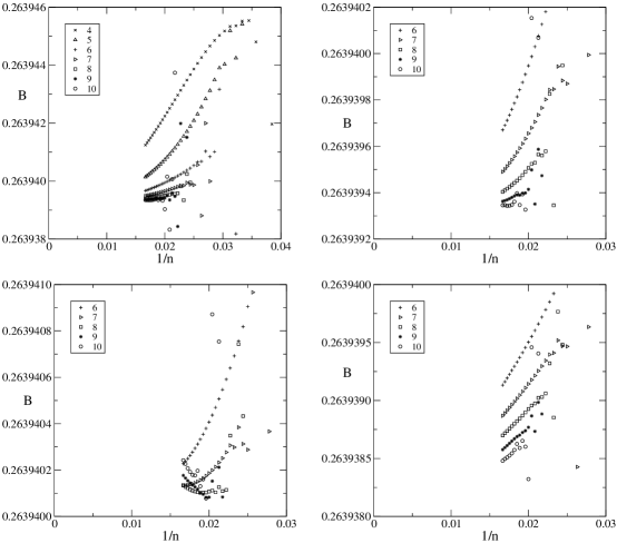
Figure 5: Estimates of the leading amplitude $B$ plotted against $1/n$ using different number of terms in the asymptotic expansion (1.1g). In the top panels we use the value $\mu=4.150797226$. The right panel just gives a more detailed look at the data shown in the left panel. In the bottom panels we use two different values $\mu=4.15079720$ (left panel) and $\mu=4.15079725$ (right panel) chosen to be at the extreme ends of our error-bounds for $\mu$.

The asymptotic form of the coefficients $r_{n}$ in the generating function for the radius of gyration was studied in [17]. The generating function (1.1a) has critical exponent $-(\alpha+2\nu)=-2$, so the leading correction-to-scaling term no longer becomes part of the analytic background term. We thus use the following asymptotic form:

$$r_{n}\sim\mu^{n}n\left[BF+\sum_{i\geq 0}a_{i}/n^{1+i/2}\right].$$ (1.1h)

We find $BF=0.013710(1)$. This is in full agreement with the predicted exact value [4] $BF=\frac{5}{32\pi^{2}}\sigma a_{0}=\frac{5\sqrt{3}}{64\pi^{2}}=0.013710424\ldots$, where, for the triangular lattice, $\sigma=1$ and $a_{0}=\sqrt{3}/2$. Combining the exact expression for $BF$ with the more accurate estimate for $B$ given above we estimate that $F=0.05194537(2)$.

The amplitudes of the area-weighted moments were studied in [31]. We fitted the coefficients to the assumed form

$$np_{n}\langle a^{k}\rangle_{n}\sim\mu^{n}n^{2k\nu+\alpha-2}k!\left[G_{k}+\sum_{i\geq 0}a_{i}/n^{1+i/2}\right],$$ (1.1i)

where the amplitude $G_{k}=G^{(k)}B/k!$ is related to the amplitude defined in equation (1.1g). The scaling function prediction for the amplitudes $G_{k}$ is [30]

$$G_{2k}B^{2k-1}=-\frac{b_{2k}}{4\pi^{3k}}\frac{(3k-2)!}{(6k-3)!},\qquad G_{2k+1}B^{2k}=\frac{b_{2k+1}}{(3k)!\pi^{3k+1}2^{6k+2}},$$ (1.1j)

where the numbers $b_{k}$ are given by the quadratic recursion

$$b_{k}+(3k-4)b_{k-1}+\frac{1}{2}\sum_{r=1}^{k-1}b_{k-r}b_{r}=0,\qquad b_{0}=1.$$ (1.1k)

We obtained [31] the results for the amplitude combinations listed in Table 7. It is clear that the estimates for the first 10 area weighted moments are in excellent agreement with the predicted exact values.

Table 7: Predicted exact values for universal amplitude combinations and estimates from enumeration data for square, hexagonal and triangular lattice polygons.

Amplitude	Exact value	Square	Hexagonal	Triangular
$B$	unknown	0.56230130(2)	1.27192995(10)	0.2639393(2)
$G_{1}$	$0.7957747\times 10^{-1}$	$0.795773(2)\times 10^{-1}$	$0.795779(5)\times 10^{-1}$	$0.795765(10)\times 10^{-1}$
$G_{2}B$	$0.3359535\times 10^{-2}$	$0.335952(2)\times 10^{-2}$	$0.335957(6)\times 10^{-2}$	$0.335947(5)\times 10^{-2}$
$G_{3}B^{2}$	$0.1002537\times 10^{-3}$	$0.100253(1)\times 10^{-3}$	$0.100255(3)\times 10^{-3}$	$0.100251(4)\times 10^{-3}$
$G_{4}B^{3}$	$0.2375534\times 10^{-5}$	$0.237552(2)\times 10^{-5}$	$0.237557(7)\times 10^{-5}$	$0.237547(6)\times 10^{-5}$
$G_{5}B^{4}$	$0.4757383\times 10^{-7}$	$0.475736(3)\times 10^{-7}$	$0.475749(10)\times 10^{-7}$	$0.475724(15)\times 10^{-7}$
$G_{6}B^{5}$	$0.8366302\times 10^{-9}$	$0.836624(5)\times 10^{-9}$	$0.836652(10)\times 10^{-9}$	$0.83660(2)\times 10^{-9}$
$G_{7}B^{6}$	$0.1325148\times 10^{-10}$	$0.132514(2)\times 10^{-10}$	$0.132519(5)\times 10^{-10}$	$0.132511(5)\times 10^{-10}$
$G_{8}B^{7}$	$0.1924196\times 10^{-12}$	$0.192418(2)\times 10^{-12}$	$0.192426(8)\times 10^{-12}$	$0.192419(8)\times 10^{-12}$
$G_{9}B^{8}$	$0.2594656\times 10^{-14}$	$0.259464(2)\times 10^{-14}$	$0.259472(12)\times 10^{-14}$	$0.25948(4)\times 10^{-14}$
$G_{10}B^{9}$	$0.3280633\times 10^{-16}$	$0.328062(4)\times 10^{-16}$	$0.328051(15)\times 10^{-16}$	$0.32812(5)\times 10^{-16}$

The amplitude ratios $D/C$ and $E/C$ were estimated by direct extrapolation of the relevant quotient sequence, using the following method [28]: Given a sequence $\{a_{n}\}$ defined for $n\geq 1$, assumed to converge to a limit $a_{\infty}$ with corrections of the form $a_{n}\sim a_{\infty}(1+b/n+\ldots)$, we first construct a new sequence $\{h_{n}\}$ defined by $h_{n}=\prod_{m=1}^{n}a_{m}$. The generating function $\sum h_{n}x^{n}\sim(1-a_{\infty}x)^{-(1+b)}$. Estimates for $a_{\infty}$ and the parameter $b$ can then be obtained from differential approximants. In this way, we obtained the estimates [1] $D/C=0.140296(6)$ and $E/C=0.439649(9)$. These amplitude estimates leads to a high precision confirmation of the CSCPS relation (1.1b) $H=0.000036(34)$.

The amplitudes of the SAW generating function and the metric properties were also studied in [1] by fitting of the coefficients to the assumed form

$$c_{n}\sim\mu^{n}n^{\gamma-1}\left[A+\sum_{i\geq 0}a_{i}/n^{1+i/2}\right],$$ (1.1l)

$$c_{n}\langle R^{2}_{e}\rangle_{n}/6\sim\mu^{n}n^{\gamma+2\nu-1}\left[AC/6+\sum_{i\geq 0}a_{i}/n^{1+i/2}\right],$$ (1.1m)

$$(n+1)^{2}c_{n}\langle R^{2}_{g}\rangle_{n}/6\sim\mu^{n}n^{\gamma+2\nu+1}\left[AD/6+\sum_{i\geq 0}a_{i}/n^{1+i/2}\right],$$ (1.1n)

$$(n+1)c_{n}\langle R^{2}_{m}\rangle_{n}/6\sim\mu^{n}n^{\gamma+2\nu}\left[AE/6+\sum_{i\geq 0}a_{i}/n^{1+i/2}\right].$$ (1.1o)

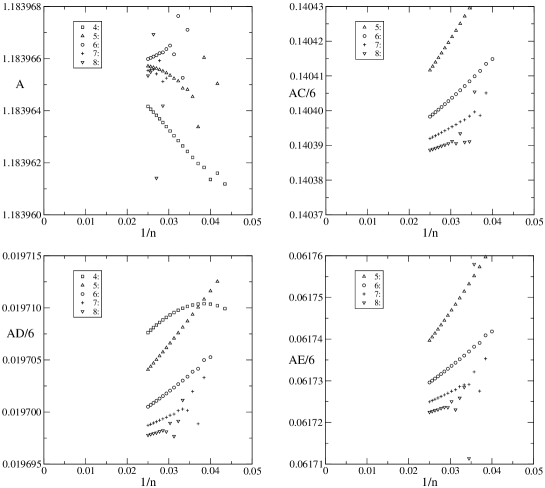
Figure 6: Estimates of the leading amplitude $A$ for SAWs, $AC/6$ for the end-to-end distance, $AD/6$ for the radius of gyration, and $AE/6$ for the monomer distance from the end-points, plotted against $1/n$ using varying number of terms in the asymptotic expansion.

In figure 6 we have plotted the estimates for the leading amplitudes against $1/n$ while varying the number of terms used in fitting to the expressions given above. From these we estimate that $A=1.183966(1)$, $AC/6=0.140380(5)$, $AD/6=0.019696(3)$, and $AE/6=0.061715(5)$. The estimate for $A$ is the same as that obtained in [1] while the remaining amplitude estimates are a little lower and have smaller error-bars that those quoted in [1]. The main reason is that here we are only interested in the leading amplitudes and base our estimates on the fits using 6-8 terms, while in [1] estimates for sub-leading amplitudes were also considered and required to be stable and consequently only fits with up to 4 terms were considered. For the metric amplitudes we thus obtain the estimates $C=0.71140(3)$, $D=0.099814(15)$, and $E=0.31275(3)$. For the universal amplitude ratios we get $D/C=0.14030(2)$ and $E/C=0.43963(5)$. We note that these estimates of the amplitude ratios are fully consistent with the more accurate estimates given above. This gives us further confidence that this method for obtaining amplitude estimates is valid. In particular, it appears, that in order to estimate the leading amplitude, we do not have to insist that estimates for sub-leading amplitudes be well converged. The smaller error-bars obtained from the fits using 6-8 terms thus appear soundly based. Naturally, some readers might wish to take a more cautious approach.

In Table 8 we have summarised estimates of various universal amplitude combinations, obtained from the work reported in this paper and elsewhere. As can be seen the estimates for all lattices are in perfect agreement strongly confirming the universality of the various combinations.

Table 8: Estimates of universal amplitude combinations on some two-dimensional lattices.

• Lattice	$D/C$	$E/C$	$BC/\sigma a_{0}$	$H$
  Square [1, 19]	0.140299(6)	0.439647(6)	0.216835(15)	-0.000024(28)
  Triangular [1]	0.140296(6)	0.439649(9)	0.216823(10)	-0.000036(34)
  Honeycomb [22]	0.1403(1)	0.4397(2)	0.2170(3)	-0.00013(67)
  Kagomé [23, 24]	0.140(1)	0.440(1)	0.2144(25)	-0.0015(47)

4 Summary and conclusion

We have presented both improved and parallel algorithms for the enumeration of self-avoiding polygons and walks on the triangular lattice. These algorithms have enabled us to obtain polygons up to perimeter length 60, their radius of gyration and area-weighted moments up to perimeter 58, while for self-avoiding walks to length 40 we calculated the number of walks as well as the metric properties of mean-square end-to-end distance, mean-square radius of gyration and the mean-square distance of a monomer from the end points.

The analysis of the polygon series enabled us to obtain a very precise estimate for the connective constant $\mu=4.150797226(26)$. We confirmed to a very high degree of accuracy the predicted exponent values $\alpha=1/2$, $\gamma=43/32$ and $\nu=3/4$. We noticed that, as is the case for the square lattice problem, the SAW asymptotics is worse behaved than the SAP asymptotics, i.e., estimates for $\mu$ and the critical exponents are at least an order of magnitude more accurate in the SAP case. It quite is possible that this behaviour is due to the leading correction-to-scaling exponent $\Delta=3/2$. In the SAP case this correction simply becomes part of the analytic background term and the SAP generating function is therefore simpler since it only has analytic corrections to scaling. We also obtained very accurate estimates for the leading amplitude of the sequence $p_{n}$ of SAP coefficients $B=0.2639393(1)$ and using the exact expression for the amplitude combination $BF$ we find $F=0.05194537(2)$. Our data for the area-weighted moments was used [31] to confirm the correctness of theoretical predictions for the values of the amplitude combinations $G^{(k)}B^{k-1}$. Finally we obtained accurate estimates for the critical amplitudes $A=1.183966(1)$, $C=0.71140(3)$, $D=0.099814(15)$, and $E=0.31275(3)$. The estimate for the ratio $C/F=13.6952(5)$ is in very good agreement with the theoretical estimate $C/F\approx 13.70$ [5]. The amplitude estimates led to a high precision confirmation of the CSCPS relation (1.1b) $H=0$.

E-mail or WWW retrieval of series

The series for the problems studied in this paper can be obtained via e-mail by sending a request to I.Jensen@ms.unimelb.edu.au or via the world wide web on the URL http://www.ms.unimelb.edu.au/~iwan/ by following the relevant links.

5 Acknowledgments

The calculations presented in this paper would not have been possible without a generous grant of computer time on the server cluster of the Australian Partnership for Advanced Computing (APAC). We also used the computational resources of the Victorian Partnership for Advanced Computing (VPAC). We gratefully acknowledge financial support from the Australian Research Council.

References

References

- [1] Caracciolo S, Guttmann A J, Jensen I, Pelissetto A, Rogers A N and Sokal A D 2004 Correction-to-scaling exponents for two-dimensional self-avoiding walks Preprint cond-mat/0409355
- [2] Caracciolo S, Pelissetto A and Sokal A D 1990 Universal distance ratios for two-dimensional self-avoiding walks: corrected conformal invariance predictions J. Phys. A: Math. Gen. 23 L969–L974
- [3] Cardy J L 1994 Mean area of self-avoiding loops Phys. Rev. Lett. 72 1580–1583
- [4] Cardy J L and Guttmann A J 1993 Universal amplitude combinations for self-avoiding walks, polygons and trails J. Phys. A: Math. Gen. 26 2485–2494
- [5] Cardy J L and Mussardo G 1993 Universal properties of self-avoiding walks from two-dimensional field theory Nucl. Phys. B 410 451–493
- [6] Cardy J L and Saleur H 1989 Universal distance ratios for two-dimensional polymers J. Phys. A: Math. Gen. 22 L601–L604
- [7] Conway A R, Enting I G and Guttmann A J 1993 Algebraic techniques for enumerating self-avoiding walks on the square lattice J. Phys. A: Math. Gen. 26 1519–1534
- [8] Conway A R and Guttmann A J 1996 Square lattice self-avoiding walks and corrections to scaling Phys. Rev. Lett. 77 5284–5287
- [9] Delest M P and Viennot G 1984 Algebraic languages and polyominoes enumeration Theor. Comput. Scie. 34 169–206
- [10] Enting I G 1980 Generating functions for enumerating self-avoiding rings on the square lattice J. Phys. A: Math. Gen. 13 3713–3722
- [11] Enting I G and Guttmann A J 1992 Self-avoiding rings on the triangular lattice J. Phys. A: Math. Gen. 25 2791–2807
- [12] Guttmann A J 1989 Asymptotic analysis of power-series expansions in Phase Transitions and Critical Phenomena (eds. C Domb and J L Lebowitz) (New York: Academic) vol. 13 pp. 1–234
- [13] Guttmann A J and Conway A R 2001 Square lattice self-avoiding walks and polygons Ann. Comb. 5 319–345
- [14] Guttmann A J and Yang Y S 1990 Universal distance ratios for 2d saws: series results J. Phys. A: Math. Gen. 23 L117–L119
- [15] Hughes B D 1995 Random Walks and Random Environments, Vol I Random Walks (Oxford: Clarendon)
- [16] Janse van Renburg E J 2000 The statistical mechanics of interacting walks, polygons, animals and vesicles (Oxford: Oxford University Press)
- [17] Jensen I 2000 Size and area of square lattice polygons J. Phys. A: Math. Gen. 33 3533–3543
- [18] Jensen I 2003 Counting polyominoes: A parallel implementation for cluster computing in Computational Science – ICCS 2003 (eds. P M A Sloot, D Abramson, A V Bogdanov, J J Dongarra, A Y Zomaya and Y E Gorbachev) (Berlin: Springer) vol. 2659 of Lecture Notes in Computer Science pp. 203–212
- [19] Jensen I 2003 A parallel algorithm for the enumeration of self-avoiding polygons on the square lattice J. Phys. A: Math. Gen. 36 5731–5745
- [20] Jensen I 2004 Enumeration of self-avoiding walks on the square lattice J. Phys. A: Math. Gen. 37 5503–5524
- [21] Jensen I and Guttmann A J 1999 Self-avoiding polygons on the square lattice J. Phys. A: Math. Gen. 32 4867–4876
- [22] Lin K Y 2000 Universal amplitude combinations for self-avoiding walks and polygons on the honeycomb lattice Physica A 275 197–206
- [23] Lin K Y and Huang J X 1995 Universal amplitude ratios for self-avoiding walks on the kagome lattice J. Phys. A: Math. Gen. 28 3641–3643
- [24] Lin K Y and Lue S J 1999 Universal amplitude combinations for self-avoiding polygons on the kagome lattice Physica A 270 453–461
- [25] Madras N and Slade G 1993 The self-avoiding walk (Boston: Birkhäuser)
- [26] Nienhuis B 1982 Exact critical point and critical exponents of O models in two dimensions Phys. Rev. Lett. 49 1062–1065
- [27] Nienhuis B 1984 Critical behavior of two-dimensional spin models and charge asymmetry in the coulomb gas J. Stat. Phys. 34 731–761
- [28] Owczarek A L, Prellberg T, Bennett-Wood D and Guttmann A J 1994 Universal distance ratios for interacting two-dimensional polymers J. Phys. A: Math. Gen. 27 L919–L925
- [29] Privman V and Redner S 1985 Tests of hyperuniversality for self-avoiding walks J. Phys. A: Math. Gen. 18 L781–L788
- [30] Richard C, Guttmann A J and Jensen I 2001 Scaling function and universal amplitude combinations for self-avoiding polygons J. Phys. A: Math. Gen. 34 L495–L501
- [31] Richard C, Jensen I and Guttmann A J 2003 Scaling function for self-avoiding polygons in Proceedings of the International Congress on Theoretical Physics TH2002 (Paris), Supplement (eds. D Iagolnitzer, V Rivasseau and J Zinn-Justin) (Basel: Birkhäuser) pp. 267–277 Preprint cond-mat/0302513