Generalized Entropies and Statistical Mechanics

Abstract

We consider the problem of defining free energy and other thermodynamic functions when the entropy is given as a general function of the probability distribution, including that for nonextensive forms. We find that the free energy, which is central to the determination of all other quantities, can be obtained uniquely numerically even when it is the root of a transcendental equation. In particular we study the cases of the Tsallis form and a new form proposed by us recently. We compare the free energy, the internal energy and the specific heat of a simple system of two energy states for each of these forms.

I Introduction

We have recently FS1 proposed a new form of nonextensive entropy which depends on a parameter similar to Tsallis entropy TS1 ; TS2 ; PA1 , and in a similar limit approaches Shannon’s classical extensive entropy. We have shown how the definition for this new form of entropy can arise naturally in terms of mixing of states in a phase cell when the cell is re-scaled, the parameter being a measure of the rescaling, and how Shannon’s coding theorem NI1 elucidates such an approach.

In this paper we shall adopt a more general attitude and try to develop the statistical mechanics of systems where the entropy is defined almost arbitrarily. Such a ’designer’ entropy LA may indeed be relevant in a specific context, but we shall not justify here any specific form. The applicability of the Tsallis form which leads to a Levy-type pdf found in many physical contexts is now well established BE1 ; CO1 ; WO1 and in the earlier paper we have commented about how our form may also be more relevant in a context that demands a more stiff pdf. In this paper we concentrate on the use of the pdf to obtain macroscopic quantities for general entropy functions.

Central to the development of the statistical mechanics of a system is the definition of the free energy, because it is related to the normalization of the probability distribution function, which in turn controls the behavior of all the macroscopic properties of the ensemble. Hence we shall first establish a general prescription to obtain the free energy, and then determine its value in a simple physical case in terms of the temperature for Tsallis and the newer form. We shall then use it to get the specific heat in both cases and see how it changes with the change of the parameter at different temperatures.

II ENTROPY AND PDF

The pdf is found by optimizing the function

$$L=S+\alpha(1-\sum_{i}p_{i})+\beta(U-\sum_{i}p_{i}E_{i})$$ (1)

where $S$ is the entropy (whichever form), $U$ the internal energy of the ensemble per constituent, $p_{i}$ is the probability of the $i$-th state which has energy $E_{i}$, and $\alpha$ and $\beta$ are the Lagrange multipliers associated with the normalization of the pdf’s $p_{i}$ and the conservation of energy.

Let us make the assumption that the entropy $S$ is a sum of the components from all the states:

$$S=\sum_{i}\phi(p_{i})$$ (2)

where $\phi$ is a generalized function which will in general be different from the Shannon form:

$$S=-\langle\log(p)\rangle\equiv-\sum_{i}p_{i}\log(p_{i})$$ (3)

We get from optimizing $L$

$$\phi^{\prime}(p)=\alpha+\beta E_{i}$$ (4)

with the simple solution

$$\phi(p_{i})=(\alpha+\beta E_{i})p_{i}$$ (5)

the constant of integration vanishing because there can be no contribution to the entropy from a state which has zero probability.

III FREE ENERGY

We shall assume that the Helmholtz free energy $A$ is defined by

$$\beta(U-A)=S$$ (6)

Hence if $S$ is nonextensive, and $U$ is extensive, then $A$ must also be nonextensive.

Using Eq.5 and Eq.6 get

$$A=-\alpha/\beta$$ (7)

Hence we get the relation for the pdf

$$p_{i}=\psi^{-1}(\beta(E_{i}-A))$$ (8)

with the definition

$$\psi(p)=\phi(p)/p$$ (9)

Here we assume that the function $\psi$ can be inverted. This may not always be the case for an arbitrary expression for the entropy, at least not in a manageable closed form. Finally, $A$ can be obtained from the constraint equation

$$\sum_{i}p_{i}=\sum_{i}\psi^{-1}(\beta(E_{i}-A))=1$$ (10)

Once $A$ has been determined, it may be placed in Eq.8 to get the pdf $p_{i}$ for each of the states, all properly normalized, and we can find $U$ and its derivative $C$, the specific heat. For the simple system that we shall be concerned with, pressure and volume, or their analogues, will not enter our considerations, and hence we have only one specific heat, $C_{v}$, with $\beta$ now identified as the inverse scale of energy, the temperature $T$,

$$C=-\beta^{2}\frac{\partial U}{\partial\beta}$$ (11)

IV SHANNON AND TSALLIS THERMODYNAMICS

The Shannon entropy Eq.3 immediately gives, using Eq.8 and Eq.9

$$p_{i}=e^{-\alpha-\beta E_{i}}=e^{\beta(A-E_{i})}$$ (12)

so that Eq.10 yields the familiar expression for $A$

$$A=-\log(Q)/\beta$$ (13)

where $Q$ is the partition function

$$Q=\sum_{i}e^{-\beta E_{i}}$$ (14)

The exponential form of $p_{i}$ in Eq.12 allows the separation of the $A$ dependent factor and hence such a simple expression for $A$ in the case of Shannon entropy, giving us normal extensive thermodynamics.

In the Tsallis case we have

$$S=-\frac{\sum_{i}p_{i}^{q}-1}{q-1}=-\langle Log_{q}(p_{i})\rangle$$ (15)

using the q-logarithm

$$Log_{q}(p)=\frac{p^{q-1}-1}{q-1}$$ (16)

and this is easily seen to lead to, using the symbol $\epsilon$ for $(1-q)$

$$p_{i}=\left(\frac{1}{1+\epsilon\beta(E_{i}-A)}\right)^{1/\epsilon}$$ (17)

We note that as it is no longer possible to separate out a common $A$ dependent factor, we can no longer find an expression for $A$ in terms of the partition function in the usual way. Instead it is necessary to solve the normalization equation Eq.10. For a general value of $\epsilon$ this will give an infinite number of roots, but for values of $\epsilon$ corresponding to reciprocals of integers, we shall have polynomial equations with a finite number of roots, which too may be complex in general. We shall later see, at least for the simple example we consider later, that a real and stable root can be found that approaches the Shannon value of $A$ as $\epsilon\rightarrow 0$, because in that limit the $Log_{q}(p)$ function in the definition of the Tsallis entropy also coincides with the natural logarithm.

V THERMODYNAMICS OF THE NEW ENTROPY

The entropy we proposed in ref.FS1 is given by

$$S=\frac{dM(q)}{dq}=-\sum_{i}p_{i}^{q}log(p_{i})$$ (18)

with mixing probability FS1

$$M(q)=1-\sum_{i}p_{i}^{q}$$ (19)

We can also express it as the q-expectation value

$$S=-\langle log(p)\rangle_{q}\equiv\sum_{i}p_{i}^{q}log(p_{i})$$ (20)

Proceeding as in the case of Tsallis entropy we get, with $\epsilon=1-q$,

$$p_{i}=e^{-W(\epsilon\beta(E_{i}-A))/\epsilon}$$ (21)

where $W$ is the Lambert function defined by

$$W(z)e^{W(z)}=z$$ (22)

Like the Tsallis case, here too we have to obtain $A$ by solving numerically the transcendental Eq. 10. For the specific heat we get

$$C=\beta^{2}\sum_{i}E_{i}(E_{i}-A)\frac{e^{-W_{i}(1+1/\epsilon)}}{1+W_{i}}$$ (23)

where we have written for brevity $W_{i}=W\left(\epsilon\beta(E_{i}-A)\right)$ and have used the following identities related to the Lambert function CO .

$$W^{\prime}(z)=\frac{W(z)}{z(1+W(z))}$$ (24)

$$W(z)/z=e^{-W(z)}$$ (25)

As $W(z)\sim z$ for small $z$, we see that for small $\epsilon$ we effectively get classical pdf and thermodynamics, as in the Tsallis case. So the parameter $\epsilon$ is again a measure of the departure from the standard statistical mechanics due to nonextensivity. However, our nonextensivity is different functionally from the Tsallis form FS1 , and the values of $\epsilon$ in the two forms can only be compared in the limit of low $\beta$. If we use the power series expansion of $W(z)$

$$W(z)=\sum_{n=1}\frac{(-n)^{n-1}z^{n}}{n!}$$ (26)

and compare that with the power series expansion for $\log(1+z)$ in a form of the Tsallis $p_{i}$ similar to the new entropy form

$$p_{i}=e^{-\log\left(1+\epsilon_{T}\beta(E_{i}-A)\right)/\epsilon_{T}}$$ (27)

we get a cancelation of the parameter $\epsilon_{n}$ of the new entropy and of Tsallis parameter $\epsilon_{T}$ in the first order, so that both distributions approach the Shannon pdf, as we have already mentioned, but if we demand equality in the second order, we get

$$\epsilon_{n}=\frac{1}{2}\epsilon_{T}$$ (28)

The third order difference between $W(Z)$ and $\log(1+z)$ is only $\frac{1}{24}z^{3}$, and hence the difference between the Tsallis form and our form of entropy will be detectable at rather low $T$, i.e. high $\beta$.

VI APPLICATION TO A SIMPLE SYSTEM

Let us consider the simplest nontrivial system, where we have only two energy eigenvalues $\pm E$, as in a spin-1/2 system. For a noninteracting ensemble of systems we shall expect the standard results PA corresponding to Shannon entropy

$$A=-\log[2\cosh(\beta E)]/\beta$$ (29)

$$S=\log[2\cosh(\beta E)]-\beta E\tanh(\beta E)$$ (30)

$$U=-E\tanh(\beta E)$$ (31)

$$C=(\beta E)^{2}/\cosh^{2}(\beta E)$$ (32)

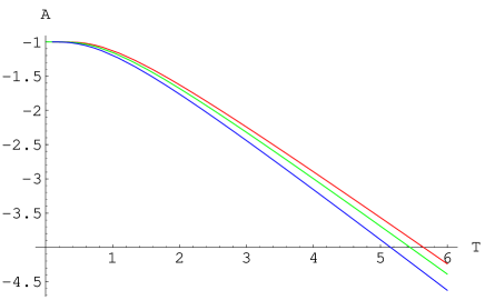
Figure 1: $A$ for Shannon (top), Tsallis with $\epsilon=0.1$ (middle) and Tsallis with $\epsilon=0.25$ (bottom)

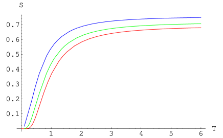
Figure 2: $S$ for same three entropy forms (from bottom to top Shannon, Tsallis (0.1), Tsallis (0.25))

For the Tsallis entropy we shall take $\epsilon=0.25,0.10$ and solve numerically. The values are shown in Figs 1-4. It is seen that Tsallis entropy gives very similar shapes for all the variables and for $\epsilon=0.10$ we get a fit much nearer to the Shannon form than for $\epsilon=0.25$.

The specific heat shows the typical Schottky form for a two-level system.

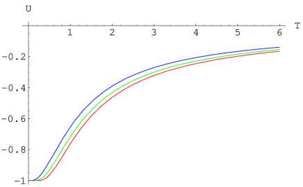
Figure 3: $U$ for same three entropy forms (same order as for $S$)

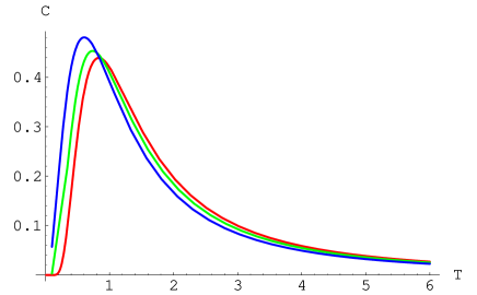
Figure 4: $C$ for same three entropy forms (peaks bottom to top - Shannon, Tsallis (0.1), Tsallis (0.25))

Though the variables involve both $p_{+}$ and $p_{-}$, after finding $A$ we can replace $p_{-}$ by $1-p_{+}$ for faster execution of the numerics.

For our new entropy too we first find the numerical value of $A$ from the normalization condition

$$e^{-W_{+}/\epsilon}+e^{-W_{-}/\epsilon}=1$$ (33)

and then use this value to find $U$, $S$, and $C$. In Figs. 5-8 we show the values corresponding to $\epsilon_{n}=0.05$, which is half the Tsallis parameter $\epsilon_{T}=0.10$ used, and also the Shannon values. We note that only for the $S$ curve we have a perceptible difference between Tsallis entropy and our new entropy at values of $\beta$ near $1$.

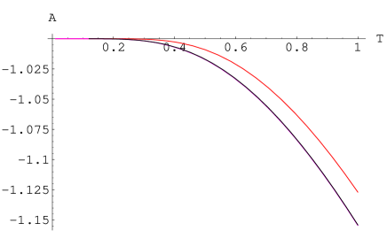
Figure 5: Comparison of $A$ for Shannon (apart), Tsallis with $\epsilon=0.1$ and new entropy for $\epsilon=0.05$ (superposed)

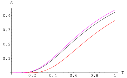
Figure 6: Comparison of $S$ for same three forms of entropy (Shannon, Tsallis (0.1), new entropy(0.05) - Tsallis is just over the new entropy ).

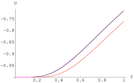
Figure 7: Comparison of $U$ for the same three entropies. Shannon is separated, other two overlap.

Figure 8: Specific heat C for same three entropies. Again, only Shannon is separated.

VII CONCLUSIONS

We have presented above a simple prescription for finding the important thermodynamic variables for any given form of the entropy as a function of the pdf’s of the states. We note that despite the apparent complexity of the exponential or transcendental equations determining the primary variable, the Helmholtz free energy $A$, it is possible to numerically get stable values which approach the expected Shannon values in the right limit of the parameter used, both in the Tsallis case and in our case of the newly defined entropy. For higher values of the parameter our entropy would give values varying significantly from the Shannon or even the Tsallis entropy, and there may be physical situations where that may indeed be the desirable characteristic. But at low values the corresponding values of the parameters for the two distributions produce virtually completely overlapping graphs. The form of the entropy may be a reflection of the effective interaction among the constituent systems of the ensemble, the Shannon form being the limiting case of the zero interaction case, and Tsallis or our form being results of different forms of interaction with $\epsilon$ standing for a coupling constant. It may be interesting to investigate more complicated systems that are physically realizable and comparable. It is noteworthy that most thermodynamic functions we have considered here are not crucially dependent on the form of the entropy with adjusted coupling, though the value of entropy itself may vary significantly in the different formulations. This probably indicates that the best way to discriminate between the suitability of different definitions of entropy in different contexts may be in comparing quantities that relate most directly to entropy.

References

- (1) F. Shafee, ”A new nonextensive entropy”, nlin.AO/0406044 (2004)
- (2) C. Tsallis,J. Stat. Phys., 52, 479(1988)
- (3) P. Grigolini, C. Tsallis and B.J. West,Chaos, Fractals and Solitons,13, 367 (2001)
- (4) A.R. Plastino and A. Plastino, J. Phys. A 27, 5707 (1994)
- (5) M.A. Nielsen and M. Chuang, Quantum computation and quantum information (Cambridge U.P., NY, 2000)
- (6) P.T. Landsberg, ”Entropies Galore”, Braz. J. Phys. 29, 46 (1999)
- (7) C. Beck, ”Nonextensive statistical mechanics and particle spectra”, hep-ph/0004225 (2000)
- (8) O. Sotolongo-Costa et al., ”A nonextensive approach to DNA breaking by ionizing radiation”, cond-mat/0201289 (2002)
- (9) C. Wolf, ”Equation of state for photons admitting Tsallis statistics”, Fizika B 11, 1 (2002)
- (10) R.M. Corless, G.H. Gonnet, D.E.G. Hare, D.J. Jeffrey and D.E. Knuth, ”On the Lambert W function”, U.W. Ontario preprint (1996)
- (11) R.K. Pathria, Statistical Mechanics, (Butterworth-Heinemann, Oxford, UK, 1996) p.77