Evolution Management in a Complex Adaptive System: Engineering the Future

Abstract

We examine the feasibility of predicting and subsequently managing the future evolution of a Complex Adaptive System. Our archetypal system mimics a competitive population of mechanical, biological, informational or human objects. We show that short-term prediction yields corridors along which the system will, with very high probability, evolve. We then show how small amounts of ‘population engineering’ can be undertaken in order to steer the system away from any undesired regimes which have been predicted. Despite the system’s many degrees of freedom and inherent stochasticity, this dynamical ‘soft’ control over future risk requires only minimal knowledge about the population’s composition.

PACS numbers: 02.50.Le, 87.23.Kg, 89.65.Ef, 05.40.2a

Complex Adaptive Systems (CAS) are of great interest to theoretical physicists because they comprise large numbers of interacting components or ‘agents’ which, unlike particles in traditional physics, may change their behavior based on past experience bocc . Such adaptation yields complicated feedback processes at the microscopic level, which in turn generate complicated global dynamics at the macroscopic level. CAS also arguably represent the ‘hard’ problem in biology, engineering, computation and sociology bocc . Depending on the application domain, the agents in CAS may represent species, people, bacteria, cells, computer hardware or software, and are typically fairly numerous, e.g. $10^{2}-10^{3}$ bocc ; 1 .

There is also great practical interest in the problem of predicting and subsequently controlling a Complex Adaptive System. Consider the enormous task facing a Complex Adaptive System ‘manager’ in charge of overseeing some complicated computational, biological, medical, sociological or even economic system. He would certainly like to be able to predict its future evolution with sufficient accuracy that he could foresee the system heading towards any ‘dangerous’ areas. However, prediction is not enough. He also needs to be able to steer the system away from this dangerous regime. Furthermore, the CAS-manager needs to be able to achieve this without detailed knowledge of the present state of its thousand different components, nor does he want to have to shut down the system completely. Instead he is seeking some form of ‘soft’ control. Unfortunately, his task looks hopeless. Even in purely deterministic systems with only a few degrees of freedom, it is well known that highly complex dynamics such as chaos can arise strogatz making both prediction and control very difficult – for example, the ‘butterfly effect’ wherein small perturbations have huge unpredictable consequences. Consequently, one would think that things would be considerably worse in a CAS, given the much larger number of interacting objects. As an additional complication, a CAS may also contain stochastic processes at the microscopic and/or macroscopic levels, thereby adding an inherently random element to the system’s dynamical evolution. The Central Limit Theorem tells us that the combined effect of a large number of stochastic processes tends fairly rapidly to a Gaussian distribution. Hence, one would guess that even with reasonably complete knowledge of the present and past states of the system, the evolution would be essentially diffusive and hence difficult to control without imposing substantial global constraints.

In this paper, we examine this question of evolution management for a simplified, yet highly non-trivial model of a CAS. We show that a surprising level of prediction and subsequent control are indeed possible. First we show that with very little knowledge about the system’s past behavior, one can produce corridors (Future-Casts) along which the system will subsequently move, characterized by their width (Characteristic Stochasticity) and their average direction (Characteristic Direction). Although these corridors evolve as the system evolves, at any particular point in time they provide an accurate prediction regarding the subsequent evolution of the system. We then show that if the Future-Cast predicts significant future risk, the system’s subsequent evolution can be steered to a safer regime via ‘population engineering’, i.e. by introducing small perturbations to the population’s heterogeneity. Despite the many degrees of freedom and inherent stochasticity both at the microscopic and macroscopic levels, this global control requires only minimal knowledge and intervention on the part of a CAS manager. For the somewhat simpler case of Cellular Automata, Israeli and Goldenfeld golden have recently obtained the remarkable result that computationally irreducible physical processes can become computationally reducible at a coarse-grained level of description. Based on our findings, one could speculate that similar ideas hold for populations of decision-taking, adaptive agents. We finish the paper by discussing a number of possible practical applications of our findings.

It is widely believed (see for example, Ref. casti1 ) that Arthur’s El Farol Bar Problem 2 provides a representative toy model for CAS’s which comprise a population of objects competing for some limited global resource (e.g. space in an overcrowded area). To make this model more complete in terms of real-world complex systems, the effect of network interconnections has recently been incorporated nets . As mentioned later, our present analysis also applies to such networked populations. The El Farol Bar Problem concerns the collective decision-making of a group of potential bar-goers (i.e. agents) who use limited global information to predict whether they should attend a potentially overcrowded bar on a given night each week. The Statistical Mechanics community has adopted a binary version of this problem, the so-called Minority Game (MG) 3 ; 6 , as a new form of Ising model which is worthy of study in its own right because of its highly non-trivial dynamics. Here we consider a generalized version of such multi-agent binary games which (a) incorporates a finite time-horizon $T$ over which agents remember their strategies’ past successes, to reflect the fact that the more recent past should have more influence than the distant past, (b) allows for fluctuations in agent numbers, since agents might only participate if they possess a strategy with a sufficiently high success rate, and (c) allows for a general reward structure thereby disposing of the MG’s restriction to automatically rewarding the minority 6 . The formalism is applicable to any CAS which can be mapped onto a population of $N$ objects which repeatedly taking actions in some form of global ‘game’. For simplicity, we restrict ourselves here to simply invoking competition for a limited resource $L$. Our model therefore incorporates the features typically associated with complex systems: strong feedback, adaptation, interconnectivity etc. At each timestep $t$, each agent makes a (binary) decision $a_{\mu(t)}$ in response to some global information $\mu(t)$. This global information is a bitstring of length $m$, and may for example represent the history of past global outcomes. The global outcome at a given timestep is based on the aggregate action of the agents and the value of the global resource level $L$. Each agent holds $k$ strategies (comprising a response to every possible history) employing the one which would have proved most successful over the last $T$ timesteps. By assigning these randomly to each agent, we mimic the effect of large-scale heterogeneity in the population. The strategy allocation is fixed at the start of the game, and can be described by a tensor of rank $k$ or ‘Quenched Disorder Matrix’ (QDM) 6 . Adding network connections simply has the effect of redistributing elements within the QDM. The agents’ aggregate action at each timestep $t$ is represented by $D(t)$, and $S(t)=S(t-1)+D(t-1)$ gives the current global output value note . Stochasticity arises via coin-tosses at both the microscopic level (to resolve an agent’s tied strategies) and the macroscopic level (to resolve any ties when deciding the global outcome). This stochasticity implies that for a given QDM, the system’s output is not unique. In short, the future evolution of the system results from the time-dependent interplay of time-dependent deterministic and stochastic processes. We refer to the set of all possible future trajectories of the game’s output at $t\geq 1$ timesteps in the future, as the Future-Cast distribution.

The game’s dynamics can be transferred into a time-horizon space $\underline{\Gamma_{t}}$ spanned by all possible combinations of the last $m+T$ global outcomes (or equivalently, the winning actions) 6 . For a binary game, $\underline{\Gamma_{t}}$ has dimension $2^{m+T}$. For any given time-horizon state $\Gamma_{t}$ in this space, there exists a unique score vector $\underline{G(t)}$ whose element $G_{R}(t)$ is the score for strategy $R$ at time $t$. Each time a particular time-horizon state is reached, the actions of the agents holding strategies whose scores are not tied, or agents holding tied strategies which prescribe the same action, will necessarily be the same. In addition, the number of remaining agents (i.e. those holding tied strategies prescribing different actions, which need to be resolved via a coin-toss) will also be the same. Subsequently, the probability distribution of $D(t)$ will be identical each time this time-horizon state occurs. The probabilities associated with the global outcomes which represent the transitions between these time-horizon states are also static. Hence it is possible to construct a Markov Chain description for the evolution of the probabilities $\underline{P(\Gamma_{t})}$ for these time-horizon states:

$$\underline{P(\Gamma_{t})}~{}=~{}\underline{\underline{T}}~{}\underline{P(\Gamma_{t-1})}.$$ (1)

The transition matrix $\underline{\underline{T}}$ is time-independent and sparse since there are only two possible global outcomes for each state. The number of non-zero elements in the matrix is thus $\leq 2^{(m+T+1)}$. These values can be generated directly from the QDM 9 . It is straightforward to obtain the stationary state solution of Eq. (1) in order to calculate the system’s time-averaged macrosopic quantities. Generating the Future-Cast probability distributions involves mapping from the internal (time-horizon) state dynamics of the system to its global output. This requires (i) the probability distribution of $D(t)$ for a given time-horizon $T$, (ii) the corresponding global outcome for a given $D(t)$, and (iii) an output generating algorithm expressed in terms of $D(t)$. We know that in the transition matrix, the probabilities represent the summation over a distribution which is binomial in the case where the agents are limited to two possible decisions. Using the output generating algorithm, we can construct an adjacency matrix $\underline{\underline{\Upsilon}}$ to the transition matrix $\underline{\underline{T}}$, with the same dimensions. The elements of $\underline{\underline{\Upsilon}}$ contain probability functions corresponding to the non-zero elements of the transition matrix, together with the discrete convolution operator. For the incremental algorithm described above, we define and use a convolution operator $\otimes$ such that $(f\otimes g)\mid_{i}~{}=\sum_{j=-\infty}^{\infty}f(i-j)\times g(j)$ (see Ref. 9 for full mathematical details). Consider an arbitrary timestep in the game, and label it as $t=0$ for convenience. The adjacency matrix can then be applied to a vector $\underline{\varsigma(S,t=0)}$, where the element of $\underline{\varsigma(S,0)}$ corresponding to the current time-horizon state comprises a probability distribution function for the current output value. Since $\underline{\varsigma(S,t)}~{}=~{}\underline{\underline{\Upsilon}}^{t}\underline{\varsigma(S,0)}$, the Future-Cast at $t$ timesteps in the future, $\Pi(S,t)$, is given by:

$$\Pi(S,t)=\sum_{i=1}^{2^{(m+T)}}\varsigma_{i}(S,t).$$ (2)

Due to the state dependence of the Markov Chain, this Future-Cast probability distribution $\Pi$ is non-Gaussian. Consider $t=1$. Since we are not interested in transients, we really need a ‘steady state’ form $\Pi_{1}=\big{<}\Pi(S,1)\big{>}_{\infty}$ representing a time-average over an infinitely long period. Fortunately, we have the steady state solutions of $\underline{P(\Gamma)}~{}=\underline{\underline{T}}~{}\underline{P(\Gamma)}$ which are the (static) probabilities of being in a given state at any time. By representing these probabilities as the appropriate functions, we can construct an initial vector $\underline{\kappa}$, which is equivalent to $\underline{\varsigma(S,0)}$ 9 . Hence we can generate the Characteristic Future-Cast $\Pi_{1}$, describing the characteristic behavior of the Future-Cast projected forward from a general time $t$, for a given QDM. The element $\kappa_{i}$ is simply the point $(0,P_{i}(\Gamma))$. Characteristic Future-Casts for any number of timesteps $t\geq 1$ into the future, can be generated by simply premultiplying $\underline{\kappa}$ by $\underline{\underline{\Upsilon}}^{t}$: i.e. use Eq. (2) with $\underline{\varsigma}~{}=~{}\underline{\underline{\Upsilon}}^{t}~{}\underline{\kappa}$. Hence the Characteristic Future-Cast over $t$ timesteps is simply the Future-Cast of length $t$ from all the $2^{m+T}$ possible initial states, with each contribution being given the appropriate weighting factor. Note that $\Pi_{t}$ is not equivalent to the convolution of $\Pi_{1}$ with itself $t$ times, and hence is not necessarily Gaussian. In other words, the Central Limit Theorem does not provide a good estimate of the future behavior of the system. The system is only quasi-diffusive at best.

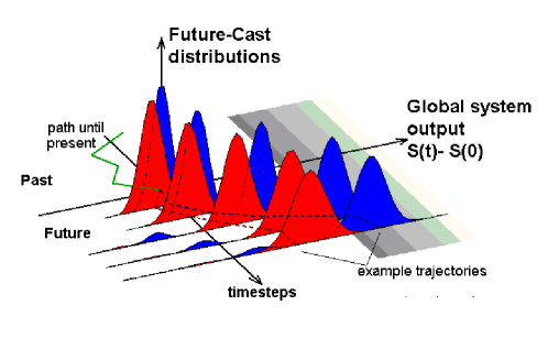
Figure 1: Evolution of the unperturbed Future-Cast probability distribution (blue solid) during a typical run of a game with the Quenched Disorder Matrix (QDM) of Fig. 2. The region of large positive deviation $S(t)$ is considered dangerous territory. Red distributions show corresponding evolution following a minor QDM perturbation (i.e. population engineering of Fig. 2) introduced at $t=0$. Examples of future trajectories also shown. Note that $t=0$ labels an arbitary timestep chosen after initial transients have disappeared.

Figure 1 shows a typical example of the evolution of the Future-Cast at $t$ timesteps ahead of the present timestep (which we label $t=0$). The Future-Cast acts to provide non-Gaussian ‘corridors’ along which the system subsequently evolves. The reason for the non-diffusive behavior is that, unlike the standard binomial paths set up during a simple coin-toss experiment, not all paths are realized at every timestep. The stochasticity generated at a given timestep, and hence the possible future paths, are conditional on the system’s past history. Now suppose that an external CAS manager decides it dangerous for the system to have a large positive $S(t)$ for $t>0$. Figure 2 shows the corresponding QDM for $t<0$, together with the QDM perturbation which the system manager decides to introduce at $t=0$. Such ‘population engineering’ can be achieved by switching on/off, rewiring or reprogramming a group of agents in a situation where the agents are accessible objects, or by introducing some form of communication channel – or even a more evolutionary approach whereby a small subset of agents (‘species’) are removed from the population and a new subset added to replace them. This evolutionary mechanism need neither be completely deterministic (i.e. knowing exactly how the form of the QDM changes) nor completely random (i.e. a random perturbation to the QDM). In this sense, it seems quite close to some modern ideas of biological evolution, whereby there is some purpose mixed with some randomness. Figure 1 shows the impact that this relatively minor perturbation has on the Future-Cast. In particular, the system gets steered ‘away from danger’ (i.e. toward smaller $S(t)$ values). Note that a substantial reduction in future risk has been achieved without needing to know the microscopic details of each agent’s individual strategies, since each QDM corresponds to a macrostate in the physical sense: i.e. it is only the aggregate number of agents holding each strategy pair which matters, not what an individual agent is holding.

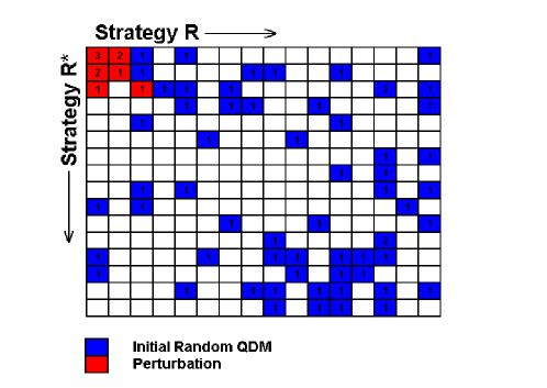
Figure 2: The unperturbed Quenched Disorder Matrix QDM (blue) and its perturbation (red) used to generate Fig. 1. The i-j coordinates represent strategy labels for the $k=2$ strategies per agent, $R$ and $R^{*}$. These binary strategies $R$ and $R^{*}$ are ordered according to their decimal equivalent. Here $m=2$. The value in each box represents the number of agents assigned that particular pair of strategies during the initial random allocation. An empty bin implies no agent holds that particular strategy pair.

Engineering an appropriate QDM perturbation involves understanding the interplay between the (i) the mean of the Future-Cast distribution, referred to as the Characteristic Direction which acts as a ‘drift’ in terms of the future output signal, and (ii) the spread in the Future-Cast distribution, referred to as the Characteristic Stochasticity which acts as ‘noise’ in terms of the future output signal. Figure 3 shows how these quantities vary for different QDMs for the illustrative case of $m=1$ with a small population. This indicates the effects of adding such a population as a perturbation to an unbiased system. In order to reliably steer $S(t)$ toward larger/smaller values, the Characteristic Direction must be much larger than the Characteristic Stochasticity. As shown, the perturbation must therefore be biased toward the upper-left/lower-right half of the QDM (but not both). This means that the perturbed population is less adaptive than the unperturbed one (i.e. more agents hold two identical strategies) and less heterogenous (i.e. more agents populate the same region of the QDM). This observation explains why the QDM perturbation of Fig. 2 had the desired steering effect shown in Fig. 1. By contrast for perturbations which are unbiased in terms of the upper-left/lower-right half of the QDM, the Characteristic Direction is zero and hence there is no net steering, while the Characteristic Stochasticity is now large. These effects can be understood in terms of Crowd-Anticrowd formation in the strategy space 3 ; 6 .

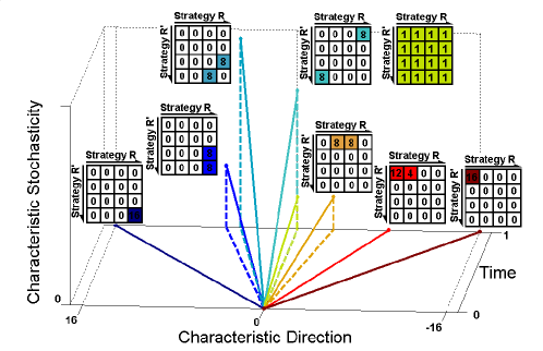
Figure 3: Characteristic Direction and Characteristic Stochasticity, for illustrative QDMs with $m=1$ and $k=2$. Results are shown for $t=1$ timesteps into the future.

Finally, we give some examples to justify why we think our Complex-Adaptive-Systems control problem is so generic. Next-generation aircraft wings may contain thousands of autonomous mini-flaps placed along the rear of a wing ilan . Denoting the binary actions of each miniflap as ‘up’ and ‘down’, and rewarding flaps for their actions given the ‘resource level’ $L$ (e.g. the plane’s current tilt), Fig. 3 shows that one can simply switch on a small number of additional miniflaps in order that the aircraft then moves autonomously in a given direction. This is achieved without requiring sophisticated control of individual miniflaps, or inter-miniflap communication ilan . In human health, there is a possible application in so-called dynamic diseases. For example, Epilepsy is a dynamic disease involving sudden changes in the activity of millions of neurons. Our work raises hopes that one could develop a relatively non-intrusive ‘brain defibrillator’ using brief electrical stimuli over a small part of the brain, rather than intrusive control over each and every one of the constituent agents (i.e. neurons). In the area of cancer therapy, the tumor to be eradicated comprises a population of cancerous and normal cells which compete for a limited resource (i.e. oxygen in blood supply, and space to grow). It is possible that by understanding how the overall tumor cell population behaves, one could do some population engineering of a small group of the malignant cells in order to steer the tumour toward benign status. Even in the immune system, where the body supposedly self-regulates itself as a result of the interaction of hundreds of different biological processes (agents), and where the corresponding ‘steering wheel’ remains unknown, our work suggests that one might be able to engineer one part of the system so that it boosts or suppresses the overall immunological activity level. In a financial setting, where intervention in a market costs money, one could imagine that an external regulator could use our analysis to steer a particular market indicator or exchange rate into a desired range without having to invest huge amounts of money. Further details of these applications will be published elsewhere. In short, we believe that the present problem lies at the heart of complex systems science both in terms of fundamental non-linear dynamical behavior and the consequences for practical safety management.

DMDS thanks Royal Bank of Scotland for funding under an EPSRC Case studentship. We are grateful to Prof. Ilan Kroo and Dr. David Wolpert for suggesting the aerospace application.

References

- (1) See N. Boccara, Modeling Complex Systems (Springer, New York, 2004) and references within, for a thorough discussion.
- (2) D.H. Wolpert, K. Wheeler and K. Tumer, Europhys. Lett. , 708 (2000).
- (3) S. Strogatz, Nonlinear Dynamics and Chaos (Addison-Wesley, Reading, 1995).
- (4) N. Israeli and N. Goldenfeld, Phys. Rev. Lett. 92, 074105 (2004).
- (5) J.L. Casti, Would-be Worlds (Wiley, New York, 1997).
- (6) B. Arthur, Amer. Econ. Rev. 84, 406 (1994); Science 284, 107 (1999); N.F. Johnson, S. Jarvis, R. Jonson, P. Cheung, Y.R. Kwong, and P.M. Hui, Physica A 258 230 (1998).
- (7) M. Anghel, Z. Toroczkai, K. E. Bassler, G. Kroniss, Phys. Rev. Lett. 92, 058701 (2004); S. Gourley, S.C. Choe, N.F. Johnson, and P.M. Hui, Europhys. Lett. (2004), in press; S. C. Choe, N. F. Johnson, and P. M. Hui, Phys. Rev. E (2004), in press; T.S. Lo, H.Y. Chan, P. M. Hui, and N. F. Johnson, Phys. Rev. E (2004) in press.
- (8) D. Challet and Y.C. Zhang, Physica A 246, 407 (1997); D. Challet, M. Marsilli, and G. Ottino, cond-mat/0306445; N.F. Johnson, S.C. Choe, S. Gourley, T. Jarrett, and P.M. Hui, in Advances in Solid State Physics Vol. 44 (Springer, Heidelberg, 2004), p. 427. See also http://www.unifr.ch/econophysics.
- (9) We originally introduced the finite time-horizon MG, plus its ‘grand canonical’ variable- and variable- generalizations, to provide a minimal model for financial markets. See M.L. Hart, P. Jefferies and N.F. Johnson, Physica A 311, 275 (2002); M.L. Hart, D. Lamper and N.F. Johnson, Physica A 316, 649 (2002); D. Lamper, S. D. Howison, and N. F. Johnson, Phys. Rev. Lett. 88, 017902 (2002); N.F. Johnson, P. Jefferies, and P.M. Hui, Financial Market Complexity (Oxford University Press, 2003). D. Challet, A. Martino, M. Marsili, I. Castillo also recently studied this finite time-horizon MG model (cond-mat/0407595).
- (10) This approach can be used to generate equivalent results for any of the system’s outputs (e.g. number of agents participating).
- (11) See I. Kroo’s work at http://aero.stanford.edu/People/kroo.html and D. Wolpert’s work at http://ic.arc.nasa.gov/dhw/.
- (12) See http://www.maths.ox.ac.uk/smithdm/transfer.pdf