Non-extensive random walks

Abstract

The stochastic properties of variables whose addition leads to $q$-Gaussian distributions $G_{q}(x)=[1+(q-1)x^{2}]_{+}^{1/(1-q)}$ (with $q\in\mathbb{R}$ and where $[f(x)]_{+}=max\{f(x),0\}$) as limit law for a large number of terms are investigated. These distributions have special relevance within the framework of non-extensive statistical mechanics, a generalization of the standard Boltzmann-Gibbs formalism, introduced by Tsallis over one decade ago. Therefore, the present findings may have important consequences for a deeper understanding of the domain of applicability of such generalization. Basically, it is shown that the random walk sequences, that are relevant to this problem, possess a simple additive-multiplicative structure commonly found in many contexts, thus justifying the ubiquity of those distributions. Furthermore, a connection is established between such sequences and the nonlinear diffusion equation $\partial_{t}\rho=\partial^{2}_{xx}\rho^{\nu}$ ($\nu\neq 1$).

Throughout the last decade increasing attention is being given to “non-extensive statistical mechanics” (NSM)[1], a theory that extends the standard Boltzmann-Gibbs one as an attempt to embrace meta-equilibrium or out-of-equilibrium regimes. The cornerstone of the non-extensive formalism is the entropy $S_{q}=k(1-\int dx[\rho(x)]^{q})/(q-1)$[2], where $k$ is a positive constant and $\rho$ a normalized probability density function (PDF) (the standard entropy is recovered in the limit $q\to 1$). Optimization of $S_{q}$, under natural constraints, leads to $q$-Gaussian s PDFs defined as

$$G_{q}(x)=G_{q}(0)[1+(q-1)x^{2}]_{+}^{\frac{1}{1-q}}\,,$$ (1)

where $q\in\mathbb{R}$, $G_{q}(0)$ is a normalization constant, and the subindex + indicates that $G_{q}(x)=0$ if the expression between brackets is non-positive. The usual Gaussian distribution is recovered in the $q\to 1$ limit. The PDF defined by Eq. (1) also contains the Cauchy and the Student’s-$t$ distributions, for $q=2$ and $q=(n+3)/(n+1)$ (where $n\in\mathbb{N}$ is the number of degrees of freedom), respectively.

The extensive research about this proposal brought to the surface the fact that many phenomena can be well described by $q$-Gaussian PDFs, from Bose-Einstein condensates [3] or defect turbulence[4] in physics to stock returns [5] in finances (see [1] for other examples). Despite the apparent ubiquity of $q$-Gaussian PDFs, giving indirect support to the applicability of NSM, a comprehensive description in terms of first principles is still at work. Nevertheless, the fact that $q$-Gaussian PDFs are so frequently found leads to think that a statistical mechanism, as for other limit distributions, may be behind. Then, assuming that sums of certain random variables fall within the basin of attraction of a given $q$-Gaussian PDF, a basic question arises: Which is the nature of such random variables? An answer to this question may give useful insights on the general framework of applicability of NSM.

Since sums of independent (or, more generally, weakly correlated) random variables lead to either the Gauss or Lévy limits [6], depending on the properties of their second moments, then the kind of stochastic variables that concern NSM are expected to have some sort of strong dependence. This idea is consistent with the nature of the systems for which NSM is supposed to apply, e.g., systems with long-range interactions or long-term memory. To visualize the particular kind of dependence involved, it may be instructive to think in terms of one-dimensional random walks, since the position of a walker at each instant is given by the summation of random variables, the individual step lengths. As a counterpart, one can also investigate the associated evolution equation for the probability density of the position of walker.

It is known that the nonlinear differential equation

$$\partial_{t}\rho={\textstyle\frac{D}{2}}\partial^{2}_{xx}\rho^{\nu}\,,$$ (2)

with $\nu,D\in\mathbb{R}$, has as time-dependent solution, for $\rho(x,0)=\delta(x)$ and natural boundary conditions[7],

$$\rho_{\nu}(x,t)=G_{2-\nu}\bigl{(}x/\alpha_{\nu}(t)\bigr{)},$$ (3)

with $G_{2-\nu}(0)\equiv g_{\nu}(t)=1/[\gamma_{\nu}\alpha_{\nu}(t)]$, $\alpha_{\nu}(t)=[\nu(\nu+1)\gamma_{\nu}^{1-\nu}Dt]^{\frac{1}{\nu+1}}$ and

$$\gamma_{\nu}=\left\{\matrix{{\displaystyle\frac{\Gamma(\frac{\nu}{\nu-1})}{\Gamma(\frac{3\nu-1}{2(\nu-1)})}}\sqrt{\frac{\pi}{\nu-1}}&\mbox{if $\nu>1$,}\cr\sqrt{\pi}&\mbox{if $\nu=1$,}\cr{\displaystyle\frac{\Gamma(\frac{\nu+1}{2(1-\nu)})}{\Gamma(\frac{1}{1-\nu})}}\sqrt{\frac{\pi}{1-\nu}}&\mbox{if $-1<\nu<1$}\,.\cr}\right.$$ (4)

The PDF defined by Eq. (3) is normalizable for $\nu>-1$ and has finite second moment for $\nu>1/3$. For $\nu>(<)0$, it must be $D>(<)0$ (see [8] for details). The Cauchy distribution corresponds to $\nu=0$, in which case there is no diffusion. However, in the limit $\nu\to 0$, diffusion can be restored by making $D\to\infty$ in such a way that $D\nu>0$ remains finite. The scaling of $x$ with time in Eq. (3) indicates superdiffusive behavior for $-1<\nu<1$, normal diffusion for $\nu=1$ and subdiffusion for $\nu>1$, although the second moment is finite only for $\nu>1/3$.

The nonlinear Fokker-Planck equation (FPE) (Eq. (2) plus a drift term) describes a variety of transport processes, such as percolation of gases through porous media [9], thin liquid films spreading under gravity [10] or spatial diffusion of biological populations [11]. L. Borland has shown that it leads to an associated Itô-Langevin equation (ILE) with multiplicative noise, where the noise amplitude is controlled by a function of the density $\rho$ [8]. In the free-particle, the ILE reads

$$\dot{x}(t)=|D|^{\frac{1}{2}}[\rho_{\nu}(x(t),t)]^{\frac{\nu-1}{2}}\eta(t),$$ (5)

where $\{\eta\}$ is a zero-mean $\delta$-correlated Gaussian process. This appears to be a very special kind of multiplicative noise that depends on the macroscopic density $\rho_{\nu}$ that, in turn, satisfies Eq. (2). Accordingly, the nonlinear FPE has been shown to be derivable from a master equation where the transition probabilities have the same power law dependence on the density $\rho$ [12]. In terms of transition rates, this means that the probability of transition from one state to another is determined by the probability of occupation of the first state. This kind of behavior is found in many systems ranging from diffusion in disordered media [9] to financial transactions [5] as discussed in Ref. [12]. Notice that, in the limit $\nu\to 1$, one recovers the standard Gaussian diffusion, with constant diffusion coefficient and transition rates.

After discretization of time in Eq. (5), the position $x_{n}$ at time $t=n\tau$ evolves according to

$$x_{n+1}=x_{n}+\sqrt{|D|\tau}[\rho_{\nu}(x_{n})]^{(\nu-1)/2}\xi_{n},$$ (6)

where the stochastic process $\{\xi\}$, obtained from $\xi_{n}=\frac{1}{\sqrt{\tau}}\int_{n\tau}^{(n+1)\tau}\eta(t){\rm d}t$, is Gaussian with $\langle\xi_{i}\rangle=0$ and $\langle\xi_{i}\xi_{j}\rangle=\delta_{ij}$. Eq. (5) represents a one-dimensional random walker with a sort of statistical feedback in which the steps depend on the local density of an ensemble of identical walkers. Fig. 1 shows the PDFs associated to the random walkers defined by Eq. (6), for different values of $\nu$. Notice that for $\nu>1$ a cut-off occurs at the points $x=\pm\alpha_{\nu}/\sqrt{\nu-1}$, as a result of the definition of the $q$-Gaussian in Eq. (1). Convergence is faster as $\nu$ approaches one.

Let us rewrite Eq. (5) by substitution of the explicit expression for $\rho_{\nu}(x,t)$ given by Eq. (3):

$$\dot{x}(t)=\sqrt{|D|}g(t)\left[1+(1-\nu)\frac{x^{2}(t)}{\alpha^{2}_{\nu}(t)}\right]^{1/2}_{+}\eta(t).$$ (7)

When $\nu\in(-1,1]$, the expression between brackets is always positive, thus, there is no cut-off. This instance corresponds to long-tailed PDFs, the case of interest in most applications. In this regime, the multiplicative noise can be interpreted as a unique effective noise for the linear stochastic equation

$$\dot{x}(t)\,=\,A_{\nu}(t)\eta_{A}(t)+x(t)M_{\nu}(t)\eta_{M}(t),$$ (8)

where

$$A_{\nu}(t) = \sqrt{|D|}[g(t)]^{\frac{\nu-1}{2}}\,,$$ (9)

$$M_{\nu}(t) = \sqrt{(1-\nu)|D|}[g(t)]^{\frac{\nu-1}{2}}/\alpha_{\nu}(t)\,,$$ (10)

and $\eta_{A}$, $\eta_{M}$ are two independent zero-mean $\delta$-correlated Gaussian noise sources with $\langle\eta_{A}(t)\eta_{A}(t^{\prime})\rangle=\langle\eta_{M}(t)\eta_{M}(t^{\prime})\rangle=\delta(t-t^{\prime})$ [13, 14].

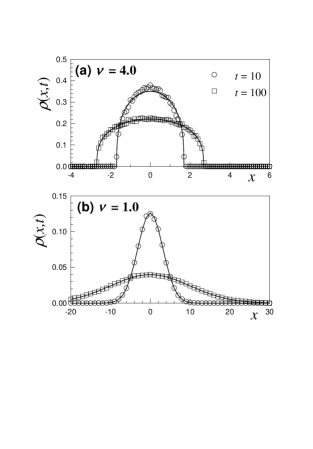
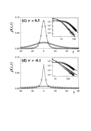
FIG. 1.: Distribution of probabilities for the position of random walkers defined by Eq. (6) together with Eq. (3), at two times indicated on the figure. (a) $\nu=4.0$ (subdiffusion), (b) $\nu=1$ (normal diffusion), (c) $\nu=0.5$ (superdiffusion) and (d) $\nu=-0.1$ (hyperdiffusion). In all cases $|D|=1$ and $\tau=10^{-1}$. Symbols correspond to the histogram built from $10^{5}$ random walkers, starting at $x_{0}=0$ (with the addition of a small noise) and solid lines to the analytical expression given by Eq. (3). Curves collapse after scaling $x$ by $t^{1/(\nu+1)}$. Insets: log-log representation to watch the tails.

In fact, both Eqs. (7) and (8) yield the same non-linear diffusion equation (2)[14]. Therefore, we have found an alternative interpretation for the nonlinear FPE and its associated ILE. Notice that, instead of two uncorrelated noises, one might consider a unique source with an appropriate time lag.

The discretized version of Eq. (8) reads

$$x_{n+1}=A_{\nu,n}\xi_{A,n}+(1+M_{\nu,n}\xi_{M,n})x_{n}\,,$$ (11)

where

$$A_{\nu,n} = \sqrt{|D|\tau}[\gamma_{\nu}^{2}(\nu+1)\nu D\tau\,n]^{\frac{1-\nu}{2(\nu+1)}}\equiv A_{\nu}n^{\frac{1-\nu}{2(\nu+1)}}\,,$$ (12)

$$M_{\nu,n} = \sqrt{(1-\nu)/[|\nu|(\nu+1)n]}\equiv\sqrt{\mu}/n^{\frac{1}{2}}\;,$$ (13)

and the independent processes $\{\xi_{A}\}$ and $\{\xi_{M}\}$ are zero-mean $\delta$-correlated Gaussian ones such that $\langle\xi_{A,i}\xi_{A,j}\rangle=\langle\xi_{M,i}\xi_{M,j}\rangle=\delta_{ij}$; as comes out after taking $\xi_{X,n}=\frac{1}{\sqrt{\tau}}\int_{n\tau}^{(n+1)\tau}\eta_{X}(t){\rm d}t$ and $X_{\nu,n}=X_{\nu}(n\tau)\sqrt{\tau}$, with $X\in\{A,M\}$. The rightmost identities in Eq. (13) define $A_{\nu}$ and $\mu$, respectively.

For $-1<\nu\leq 1$, the walkers given by Eqs. (6) and (11) are equivalent. In fact, it was numerically verified that Eq. (11) yields the same PDFs shown in Fig. 1(c)-(d), which were built from Eq. (6). These PDFs are stable through scaling by $n^{\frac{1}{\nu+1}}$. Notice that while $A_{\nu,n}$ increases with $n$, $M_{\nu,n}$ decreases. In the particular case $\nu=1$, one recovers the purely additive random process, with a time-independent coefficient $A_{\nu}$, i.e., $x_{n+1}\;=\;x_{n}\,+\,A_{\nu}\xi_{n}$.

The linear character of expression (11) provides the advantage of obtaining, by recurrence, an explicit formula for the position of the walker, in terms of the random sequences $\{\xi_{A}\}$ and $\{\xi_{M}\}$, namely,

$$x_{n+1} = x_{0}\prod_{i=0}^{n}(1+M_{\nu,i}\xi_{M,i})+$$ (15)

$$\;\;\;\;\;\;\;\;+\sum_{j=0}^{n}A_{\nu,j}\xi_{A,j}\prod_{i=j+1}^{n}(1+M_{\nu,i}\xi_{M,i})\,.$$

In the case $\nu>1$, nonlinearity subsists due to the cut-off condition and, therefore, it is not possible to obtain a closed form expression as above. When $\nu=1$, the product equals one (since $M_{1,i}$=0 for all $i$), coefficients $A_{1,j}$ are constant, and $x_{n}$ scaled by $n^{1/2}$ tends in distribution to a stable normal distribution, in agreement with the standard central limit theorem. However, as we have seen, in the cases $\nu\neq 1$, the distribution of the sum $x_{n}$, scaled by $n^{1/(\nu+1)}$, tends to a stable $(2-\nu)$-Gaussian.

The position of the walker at time $n\tau$, $x_{n}$, can also be written as the sum $x_{n}=x_{0}+\sum_{j=0}^{n-1}s_{j}$ , where the step length at time $\j\tau$,

$$s_{j}\equiv x_{j+1}-x_{j}=A_{\nu,j}\xi_{A,j}+M_{\nu,j}\xi_{M,j}x_{j}\,,$$ (16)

is somewhat modulated by the full history of the walker. Notice that the increments have also a sort of memory of the initial condition, through $x_{j}$ (see Eq. (15)). For simplicity, in what follows, we will take $x_{0}=0$. Recalling that the variables $\{\xi_{A}\}$ and $\{\xi_{M}\}$ are uncorrelated, and noticing that $\langle s_{j}\rangle=0$, then, the two-time correlation of the increments is

$$\langle s_{j}s_{j^{\prime}}\rangle=\delta_{jj^{\prime}}(A^{2}_{\nu,j}+M^{2}_{\nu,j}\langle x^{2}_{j}\rangle)\,,$$ (17)

where, from Eqs. (13) and (15)

$$\langle x^{2}_{j}\rangle = \sum_{k=0}^{j-1}A^{2}_{\nu,k}\prod_{i=k+1}^{j-1}(1+M^{2}_{\nu,i})\frac{k!\,k^{\frac{1-\nu}{\nu+1}}}{\Gamma(k+\mu+1)}$$ (18)

$$= A^{2}_{\nu}\frac{\Gamma(j+\mu)}{(j-1)!}\sum_{k=0}^{j-1}\frac{k!\,k^{\frac{1-\nu}{\nu+1}}}{\Gamma(k+\mu+1)}\,.$$ (19)

By means of the Stirling approximation, for large $j$ and $\nu>1/3$, one obtains $\langle x^{2}_{j}\rangle=\alpha^{2}_{\nu}(j\tau)/(3\nu-1)$. This expression coincides with $\langle x^{2}\rangle=\int x^{2}\rho_{\nu}(x,t){\rm d}x=\alpha^{2}_{\nu}(t)/(3\nu-1)$, where $t=j\tau$. For $\nu\leq 1/3$, the Stirling formula yields $\langle x^{2}_{j}\rangle=\phi(\nu)\alpha^{2}_{\nu}(j\tau)j^{\frac{1-\nu-2|\nu|}{|\nu|(\nu+1)}}$, where $\phi(\nu)$ is a function of $\nu$ only, that goes to 1 when $\nu(\nu+1)\to 0$ and diverges at $\nu=1/3$. This result is compatible with the fact that $\langle x^{2}\rangle$ is divergent in this case, as there is an the additional increase of $\langle x^{2}_{j}\rangle/\alpha^{2}(j\tau)$ given by the factor with positive power of $j$. The divergence is logarithmic at the marginal case $\nu=1/3$.

In particular, the increments $s_{j}$ are $\delta$-correlated, in accord with a Hurst exponent $H=1/2$ previously found [8]. For large $j$, Eq. (17) leads to

$$\langle s^{2}_{j}\rangle=\frac{2\alpha_{\nu}^{2}(j\tau)}{(\nu+1)(3\nu-1)j}\sim j^{\frac{1-\nu}{1+\nu}}$$ (20)

for $\nu>1/3$, and a divergent second moment for $\nu\leq 1/3$. It is easy to verify, in the former case, that $\langle x^{2}_{n}\rangle=\sum_{j=0}^{n-1}\langle s^{2}_{j}\rangle$, as it must be for a sum of uncorrelated variables. Moreover, $max_{j}[\langle s^{2}_{j}\rangle/\langle x^{2}_{n}\rangle]\sim 1/n$, thus, none of the steps gives a predominant contribution to the dispersion of the sum.

However, higher order moments of the steps do not generically factorize. For instance, $\langle s_{j}^{2}s_{j^{\prime}}^{2}\rangle\neq\langle s_{j}^{2}\rangle\langle s_{j^{\prime}}^{2}\rangle$. Therefore, the steps are not mutually independent although uncorrelated. This is why the present sums do not converge in distribution to the Gauss nor Lévy limiting laws.

Perhaps, more interesting, are akin processes with time-independent coefficients. They are associated to a nonlinear FPE with linear drift and yield steady states of the $q$-Gaussian form [14, 15]. Namely, the stochastic Itô-Langevin equation

$$\dot{u} = -\gamma u\,+\,A\,\eta_{A}(t)\,+\,uM\,\eta_{M}(t)$$ (21)

$$= -\gamma u\,+\,[A^{2}+M^{2}u^{2}]^{\frac{1}{2}}\eta(t),$$ (22)

with $\gamma\in\mathbb{R}$, $A,M$ positive constants, and the processes $\{\eta_{A}\}$, $\{\eta_{M}\}$ and $\{\eta\}$ defined as above, is associated to the following FPE[14]

$$\partial_{t}\rho=\gamma\partial_{u}[u\rho]+{\textstyle\frac{1}{2}}\partial^{2}_{uu}([A^{2}+M^{2}u^{2}]\rho)\;.$$ (23)

Its stationary solution is $\rho_{\nu}^{s}(u)=G_{2-\nu}(u/\beta_{\nu})$, with $\nu=\gamma/(\gamma+M^{2})\leq 1$, $\beta_{\nu}=\sqrt{1-\nu}\,A/M$ and $G_{2-\nu}(0)\equiv g_{\nu}=1/(\beta_{\nu}\gamma_{\nu})$. The FPE (23) can be cast in the form

$$\partial_{t}\rho=\gamma\partial_{u}(u\rho)+{\textstyle\frac{D}{2}}\partial^{2}_{uu}([\rho_{\nu}^{s}(u)]^{\nu-1}\rho)\;,$$ (24)

where $|D|=A^{2}g_{\nu}^{1-\nu}$. Then, in this case, the diffusion coefficient depends on a power of the long-time solution.

Time discretization in Eq. (22) leads to

$$u_{n+1}=\bar{A}\xi_{A,n}+(1-\kappa+\bar{M}\xi_{M,n})u_{n}\,,$$ (25)

where the processes $\{\xi_{A}\}$ and $\{\xi_{M}\}$ are the same as before, $\kappa=\gamma\tau$, $\bar{A}=A\sqrt{\tau}$ and $\bar{M}=M\sqrt{\tau}$. Taking $u_{0}=0$, and proceeding as for the first walker, the variance is

$$\langle u^{2}_{n}\rangle\,=\,\bar{A}^{2}\sum_{k=0}^{n-1}\prod_{i=k+1}^{n-1}\Lambda\,=\,\bar{A}^{2}\sum_{k=0}^{n-1}\Lambda^{n-k-1}\,,$$ (26)

where $\Lambda=(1-\kappa)^{2}+\bar{M}^{2}$. In the limit of large $n$ (and small $\tau$), $\langle u^{2}_{n}\rangle$ coincides with $\int u^{2}\rho^{(s)}_{\nu}(u){\rm d}u=\beta^{2}_{\nu}/(3\nu-1)=A^{2}/(2\gamma-M^{2})$, for $\nu>1/3$ (hence, $\Lambda<1$), and diverges otherwise (because $\Lambda\geq 1$).

Since the stationary distribution is a $(2-\nu)$-Gaussian, this PDF represents the limit law for the random walker with constant coefficients. That is, the $(2-\nu)$-Gaussian is the stable distribution of $u_{n}$ (without further scaling), for sufficiently large $n$. Stability is illustrated in Fig. 1. The constant $\bar{M}^{2}/\kappa=M^{2}/\gamma$ determines the tail law, through the value of $\nu$, while $\bar{A}/\bar{M}=A/M$ determines the width of the limit distribution. In this case increments

$$r_{j}\equiv u_{j+1}-u_{j}=\bar{A}\xi_{A,j}+(-\kappa+\bar{M}\xi_{M,j})u_{j}$$ (27)

are correlated and history-dependent, as soon as $\kappa\neq 0$. Because coefficients are not time-dependent, the underlying mechanisms are more evident in this case.

Summarizing, we have characterized the random variables whose addition has a $q$-Gaussian as limit distribution. We considered (i) a purely diffusive situation, where the density spreads out, and (ii) a case with external linear drift, where a steady density is attained. In both cases, the increments originate from two sequences of independent, identically distributed Gaussian variables $\{\xi_{A}\}$ and $\{\xi_{M}\}$, the first acting additively and the other through a linear multiplicative contribution. This structure yields a different limit law that the strictly additive one that leads to the usual Gauss or Lévy limits. The resulting increments are non-identically distributed random variables with null correlation in the former case and correlated in the latter. The existence of limit laws for similar additive-multiplicative processes has been detected before but explicit expressions for the PDFs were not found[16]. In conclusion, the ubiquity of $q$-Gaussian PDFs cannot be surprising as far as additive-multiplicative structured sequences are in fact frequent in several contexts[17].

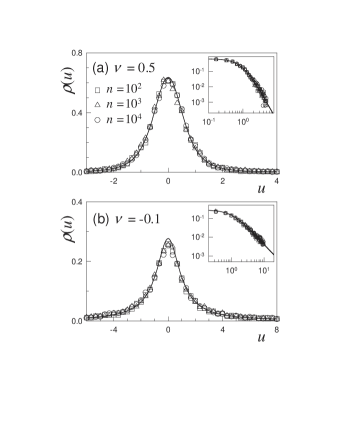
FIG. 2.: Distribution of probabilities for the position of random walkers defined by Eq. (25), for three values of the number of steps $n$, indicated on the figure. Parameters are (a) $(A/M,M^{2}/\gamma,\tau)=(1,1,0.01)$, hence $\nu=0.5$; (b) $(A/M,M^{2}/\gamma,\tau)=(1,-11,0.01)$, hence $\nu=-0.1$. Symbols correspond to histograms built from $10^{4}$ random walkers, starting at $u_{0}=0$, and solid lines to $G_{2-\nu}(u/\beta_{\nu})$ with $\beta_{\nu}=\sqrt{1-\nu}A/M$. Insets: log-log representation to watch the tails.

Following the lines of Ref. [14], the present approach could be extended to PDFs of a more general form than the $q$-Gaussian, as for instance $\rho=[1+(q-1)x^{\mu}]_{+}^{1/(1-q)}$, with $\mu\neq 2$, also frequently found [1].

I am grateful to E.M.F. Curado, S.M.D. Queirós, A.M.C. de Souza and C. Tsallis for interesting observations.

REFERENCES

- [1] Nonextensive Statistical Mechanics and its Applications, edited by S. Abe and Y. Okamoto, Lecture Notes in Physics Vol. 560 (Springer-Verlag, Heidelberg, 2001); Non-Extensive Thermodynamics and Physical Applications, edited by G. Kaniadakis, M. Lissia, and A. Rapisarda [Physica A 305 (2002)]; Anomalous Distributions, Nonlinear Dynamics and Nonextensivity, edited by H. L. Swinney and C. Tsallis [Physica D 193 (2004)]. Nonextensive Entropy - Interdisciplinary Applications, edited by M. Gell-Mann and C. Tsallis (Oxford University Press, New York, 2004).
- [2] C. Tsallis, J. Stat. Phys. 52, 479 (1988).
- [3] K.S. Fa et al., Phys. A 295, 242 (2001); E. Erdemir and B. Tanatar, Phys. A 322, 449 (2003).
- [4] K.E. Daniels, C. Beck and E.B. Bodenschatz, Physica D 193, 208 (2004).
- [5] L. Borland, Phys. Rev. Lett. 89, 098701 (2002); C. Tsallis, C. Anteneodo, L. Borland and R. Osorio, Physica A 324, 89 (2003);
- [6] W. Feller, An introduction to probability theory and its applications V. 1,2 (Wiley, New York, 1968); P. Lévy, Théorie de l’addition des variables aléatoires (Gauthier-Villars, Paris, 1954); Processus stochastiques et mouvement brownien (Gauthier-Villars, Paris, 1948); J.P. Bouchaud and A. Georges, Phys. Rep. 195, 127 (1990).
- [7] C. Tsallis and D.J. Burkman, Phys. Rev. E 54, 1 (1996); L.A. Peletier in Applications of nonlinear analysis in the physical sciences (Pitman, Massachusetts, 1981); M. Muskat, The flow of homogeneous fluids through porous media (McGraw-Hill, New York, 1937); D. H. Zanette, Braz. J. Phys. 29, 108 (1999).
- [8] L. Borland, Phys. Rev. E 57, 6634 (1998).
- [9] H. Spohn, J. Phys. I 3, 69 (1993).
- [10] J. Buckmaster, Fuid. Mech. 81, 735 (1977).
- [11] M.E. Gurtin and R.C. MacCamy, Math. Biosci. 33, 35 (1977).
- [12] E.M.F. Curado and F.D. Nobre, Phys. Rev. E 67, 021107 (2003); F.D. Nobre, E.M.F. Curado and G. Rowlands, Physica A 334, 109 (2004).
- [13] H. Risken, The Fokker-Planck Equation. Methods of Solution and Applications (Springer-Verlag, New York, 1984); C. W. Gardiner, Handbook of Stochastic Methods, (Springer, Berlin, 1994).
- [14] C. Anteneodo and C. Tsallis, J. Math. Phys. 44, 5194 (2003).
- [15] H. Sakaguchi, J. Phys. Soc. Jpn 70, 3247 (2001).
- [16] A.S. Paulson and V.R.R. Uppuluri, Math. Biosci. 13, 325 (1972).
- [17] H. Kesten, Acta Math. 131, 207 (1973), and references there in.