Critical dynamics and global persistence in a probabilistic three-states cellular automaton

Abstract

In this work a three-states cellular automaton proposed to describe part of a biological immune system tome96 is revisited. We obtain the dynamic critical exponent $z$ of the model by means of a recent technique that mixes different initial conditions. Moreover, by using two distinct approaches, we have also calculated the global persistence exponent $\theta_{g}$, related to the probability that the order parameter of the model does not change its sign up to time $t$ [$P(t)\propto t^{-\theta_{g}}$].

I Introduction

Cellular automata are statistical-mechanical models which present a complex behavior, despite their relatively simple dynamic rules. In general these models are defined in $d$-dimensional lattices with linear dimension $L$, in which each site $i$ $(1\leq i\leq L^{d})$ is occupied by a variable $s_{i}$. The dynamic rules of a typical cellular automaton have two basic characteristics: Firstly, the update of a variable $s_{i}$ depends only on its neighborhood (short-range interactions). Secondly, given a configuration of the system at instant $t$, at instant $t+1$ all variables $s_{i}$ $(1\leq i\leq L^{d})$ are updated at once. The use of cellular automata in order to mimic biological immune systems has improved the understanding about the microscopic mechanisms that lead to the macroscopic behavior of these systems bezzi01 . For example, cellular automata are as usefull to describe the T-helper cells response under parasitic infections brass94 ; brass94a as they are to model the course of the Human Immunodeficiency Virus (HIV) infection zorzenon01 .

Brass et al. divised a simple cellular automaton model of $\mbox{T}_{\mbox{\scriptsize H}}$ cell interactions to mimic the immune system of mice exposed to parasitic infections brass94 ; brass94a . The model is defined in a cubic ($d=3$) lattice in which each site is occupied by one of three different $\mbox{T}_{\mbox{\scriptsize H}}$ cell types: $\mbox{T}_{\mbox{\scriptsize H}}0$, $\mbox{T}_{\mbox{\scriptsize H}}1$ and $\mbox{T}_{\mbox{\scriptsize H}}2$ cells. T-helper cells that have not yet been presented to the antigen are denoted by $\mbox{T}_{\mbox{\scriptsize H}}0$. In the model, two distinct routes (equivalent to two populations of antigen presenting cells) govern the maturing of a $\mbox{T}_{\mbox{\scriptsize H}}0$ cell: Antigen presented by the first (second) route elicit a $\mbox{T}_{\mbox{\scriptsize H}}1$ ($\mbox{T}_{\mbox{\scriptsize H}}2$) response. In order to take into account the competition between mature $\mbox{T}_{\mbox{\scriptsize H}}$ cells, the induction $\mbox{T}_{\mbox{\scriptsize H}}0\rightarrow\mbox{T}_{\mbox{\scriptsize H}}1$ ($\mbox{T}_{\mbox{\scriptsize H}}2$) is forbidden when the neighborhood of the $\mbox{T}_{\mbox{\scriptsize H}}0$ cell has an overall majority of $\mbox{T}_{\mbox{\scriptsize H}}2$ ($\mbox{T}_{\mbox{\scriptsize H}}1$) cells. At last, a mature cell dies (it is substituted by a $\mbox{T}_{\mbox{\scriptsize H}}0$ cell) if such a cell is not restimulated by the appropriate antigen within the time interval $N_{T}$. The model can display a spontaneous symmetry breaking as one varies the antigen density or the cutoff $N_{T}$, in agreement with experimental results else93 . A probabilistic version of the model was proposed by Tomé and Drugowich de Felício tome96 by allowing the death of cells $\mbox{T}_{\mbox{\scriptsize H}}1$ and $\mbox{T}_{\mbox{\scriptsize H}}2$ at each time step with a probability $r$. Thus, in this modified version of the model, the lifetime $N_{T}$ was substituted by a mean lifetime related to the probability $r$. Also, the development of $\mbox{T}_{\mbox{\scriptsize H}}0$ cells into either $\mbox{T}_{\mbox{\scriptsize H}}1$ or $\mbox{T}_{\mbox{\scriptsize H}}2$ cells occurs with a probability that depends on the neghborhood of the $\mbox{T}_{\mbox{\scriptsize H}}0$ cell and on a parameter $p$, related to the antigen density. Such probabilistic version presents the intrinsic spontaneous symmetry breaking found in the Brass et al. automaton, besides being amenable to an analytical approach tome96 . The critical behavior of the probabilistic model proposed in Ref. tome96 was studied in a subsequent work by Ortega et al. ortega98 . By using a finite-size scaling analysis, from Monte Carlo simulations of square lattices, Ortega et al. determined the ratios of exponents $\frac{\beta}{\nu}$ and $\frac{\gamma}{\nu}$, as well as the critical point of the model. Their results suggest that the probabilistic automaton, although not satisfying detailed balance, belongs to the same universality class of the two-dimensional kinetic Ising model ortega98 , thus supporting the up-down conjecture, introduced by Grinstein et al. grinstein85 . In a subsequent work, Tomé and Drugowich tome98 obtained the dynamic critical exponent $z$ of the probabilistic automaton in two dimensions, by performing short-time Monte Carlo simulations by studying the collapse of the fourth order Binder’s cumulant for different lattice sizes.

In the present work we have revisited the probabilistic automaton of Ref. tome96 . We have re-obtained the dynamic critical exponent $z$ of the automaton by using a recent technique that mixes different initial conditions dasilva02 . Such technique is based upon the short-time critical dynamics introduced by Janssen et al. janssen89 , who showed that even far from equilibrium the short-time relaxation of the order parameter follows a universal scale form

$$M(t)=m_{0}t^{\theta},$$ (1)

where $M(t)$ is the order parameter at instant $t$ (measured in Monte Carlo steps per Spin - MCS), $m_{0}=M(0)$ is a small initial $(t=0)$ value of the order parameter, and $\theta$ is the dynamic critical exponent, related to the increasing of the order parameter after the quenching of the system (When dealing with Monte Carlo simulations, the time $t$ is discrete and measured in Monte Carlo Steps per Spin - MCS). Eq. (1) demands working with sharply prepared initial states with a precise value of $m_{0}$. After obtaining the critical exponent $\theta$ for a number of $m_{0}$ values, the final value for $\theta$ is obtained from the limit $m_{0}\rightarrow 0$.

Starting from an ordered state $(m_{0}=1)$, the order parameter $M(t)$ decays in time, at the critical temperature, according to the power law zheng98

$$\langle M(t)\rangle_{m_{0}=1}\sim t^{-\beta/\nu z},$$ (2)

where $\langle(\cdots)\rangle$ is the average of the quantity $(\cdots)$ over different samples with initial order parameter value $m_{0}=M(0)$, $\beta$ and $\nu$ are the usual static critical exponents, related to the order parameter and to the correlation length, respectively, and $z$ is the dynamic critical exponent, defined as $\tau\sim\xi^{z}$, where $\tau$ and $\xi$ are time and spatial correlation lengths, respectively.

Starting from a disordered configuration with $m_{0}=0$, the second moment of the order parameter increases after the power law

$$\langle M^{2}(t)\rangle_{m_{0}=0}\sim t^{\omega},$$ (3)

where the exponent $\omega$ is given by

$$\omega=\left(d-\frac{2\beta}{\nu}\right)\frac{1}{z},$$ (4)

and $d$ is the dimension of the system.

By combining Eqs. (2) and (3), da Silva et al. dasilva02 obtained the ratio

$$F_{2}=\frac{\langle M(t)^{2}\rangle_{m_{0}=0}}{\langle M(t)\rangle^{2}_{m_{0}=1}}\sim t^{d/z},$$ (5)

which corresponds to a function with mixed initial conditions. At this point, it is important to stress here that, from Eq. (5) above, two independent runs are necessary in order to calculate the ratio $F_{2}$: In one of them $m_{0}=0$ (numerator), while in the other one $m_{0}=1$ (denominator). The ratio $F_{2}$ has proven to be useful in determining the exponent $z$, according to recent studies of the 2D Ising model dasilva02 , $q=3$ and $q=4$ states Potts models dasilva02 , Ising model with next-nearest-neighbor interactions alvesjr03 , Baxter-Wu model arashiro03 , at the tricritical point of the 2D Blume-Capel model dasilva02a , at the Lifshitz point of the 3D ANNNI model alvesjr04 and in other studies concerning models with one absorbent state dasilva04 .

In addition, in this work we have also calculated the global persistence exponent $\theta_{g}$ majumdar96 , related to the probability that the order parameter of the model, $M(t)$, does not change its sign up to time $t$, after a quench of the system to the critical temperature.

The layout of this paper is as follows: In section II we explain the model. In section III we define the order parameter $M(t)$ and we describe the methodology used in order to obtain the dynamic critical exponents $\theta_{g}$ and $z$. In section IV the results obtained for the exponents $z$ and $\theta_{g}$ are shown. Finally, in section V we present the main concluding remarks.

II The model

In this work we have studied a two-dimensional probabilistic cellular automaton in which dynamics is governed by local stochastic rules. At each site $i$ of the square lattice we have attached a variable $\sigma_{i}$ assuming the value $0,+1$ or $-1$, depending on whether the site is occupied by a $\mbox{T}_{\mbox{\scriptsize H}}0$, a $\mbox{T}_{\mbox{\scriptsize H}}1$ or a $\mbox{T}_{\mbox{\scriptsize H}}2$ cell, respectively. Considering $N$ the total number of sites in the lattice, we have defined the set $\sigma=(\sigma_{1},\sigma_{2},\cdots,\sigma_{N})$ to represent the microscopic state of the system.

The probability of state $\sigma$ at time $t$, $P_{t}(\sigma)$, evolves in time according to the equation

$$P_{t+1}(\sigma^{\prime})=\sum_{\sigma}W(\sigma^{\prime}|\sigma)P_{t}(\sigma),$$ (6)

where the transition probability $W(\sigma^{\prime}|\sigma)$ from state $\sigma$ to state $\sigma^{\prime}$ obeys the condition

$$\sum_{\sigma^{\prime}}W(\sigma^{\prime}|\sigma)=1.$$ (7)

On the other hand, for a system that evolves at discrete time steps, in which all the sites are updated at once, as is the case for the cellular automaton in this work, the transition probability $W(\sigma^{\prime}|\sigma)$ is written in the form

$$W(\sigma^{\prime}|\sigma)=\prod_{i=1}^{N}\omega_{i}(\sigma_{i}^{\prime}|\sigma),$$ (8)

where $\omega_{i}(\sigma_{i}^{\prime}|\sigma)$ is the conditional probability that site $i$ be in the state $\sigma_{i}^{\prime}$ at time $t+1$, given that the state of the system is $\sigma$ at instant $t$. Such conditional probability satisfies the condition

$$\sum_{\sigma_{i}^{\prime}}\omega_{i}(\sigma_{i}^{\prime}|\sigma)=1,$$ (9)

what implies immediately that Eq. (7) is fulfilled. The cellular automaton investigated in this work belongs to the class of totalistic cellular automata wolfram83 . Thus, the transition probability $\omega_{i}(\sigma_{i}^{\prime}|\sigma)$ depends on $\sigma_{i}$ and on the sum $\xi=\sum_{\delta}\sigma_{i+\delta}$, where the sum runs over the neighborhood of site $i$. More specifically, we are considering a particular kind of totalistic automaton for which $\omega_{i}(\sigma_{i}^{\prime}|\sigma)$ depends only on the sign of the sum $\xi$. By defining

$$s_{i}=\mbox{sign}(\xi)=\left\{\begin{array}[]{lll}\ \ 1&\mbox{if}&\xi>0,\\ \ \ 0&\mbox{if}&\xi=0,\\ -1&\mbox{if}&\xi<0,\end{array}\right.$$ (10)

we may use the notation $\omega_{i}(\sigma_{i}^{\prime}|\sigma_{i},s_{i})$ in order to explicit the transition probability dependence on $\sigma_{i}$ and $s_{i}$.

The transition probabilities (dynamical rules) are given by

$$\omega_{i}(+1|\sigma_{i},s_{i})=p\delta(\sigma_{i},0)\{\delta(s_{i},+1)+\frac{1}{2}\delta(s_{i},0)\}+(1-r)\delta(\sigma_{i},+1),$$ (11)

$$\omega_{i}(-1|\sigma_{i},s_{i})=p\delta(\sigma_{i},0)\{\delta(s_{i},-1)+\frac{1}{2}\delta(s_{i},0)\}+(1-r)\delta(\sigma_{i},-1),$$ (12)

$$\omega_{i}(0|\sigma_{i},s_{i})=(1-p)\delta(\sigma_{i},0)+r\{\delta(\sigma_{i},+1)+\delta(\sigma_{i},-1)\},$$ (13)

where, as discussed in section I, $r$ is the death probability of $\mbox{T}_{\mbox{\scriptsize H}}1$ and $\mbox{T}_{\mbox{\scriptsize H}}2$ cells, and $p$ is a parameter related to the antigen density tome96 .

The dynamical rules (11), (12) and (13 ) above have “up-down”, i.e.,

$$\omega_{i}(\sigma_{i}^{\prime}|\sigma_{i},s_{i})=\omega_{i}(-\sigma_{i}^{\prime}|-\sigma_{i},-s_{i}).$$ (14)

Therefore, following Grinstein et al. grinstein85 , we expect that the probabilistic cellular automaton investigated in this work be at the same universality class of kinetic Ising models.

III The order parameter and the dynamic exponent $\theta_{g}$

III.1 Order parameter

In the short-time Monte Carlo simulations performed in this work the order parameter $M(t)$, as well as its higher moments $M^{(k)}(t)$, were obtained from averages over a certain number of samples, $N_{s}$. By defining the $k$th momentum of the order parameter in sample number $j$ at instant $t$ as

$$M_{j}^{k}(t)=\frac{1}{L^{2k}}\left(\sum\limits_{i=1}^{L^{2}}\sigma_{ij}(t)\right)^{k},$$ (15)

the order parameter is written in the form

$$M^{(k)}(t)=\left\langle M_{j}^{k}(t)\right\rangle=\frac{1}{N_{s}L^{2k}}\sum\limits_{j=1}^{N_{s}}\left(\sum\limits_{i=1}^{L^{2}}\sigma_{ij}(t)\right)^{k}.$$ (16)

As defined in Eqs. (15) and (16) above, for $k=1$ the order parameter is exactly the mean magnetization, $M^{(1)}(t)=\left\langle M(t)\right\rangle$.

Eq. (16) defines the order parameter and its higher moments for a set of $N_{s}$ samples. Thus, if $N_{b}$ sets of samples are considered at instant $t$, there are $N_{b}$ measurements of the magnetization (and its higher moments), $M_{l}^{(k)}(t)$, where $1\leq l\leq N_{b}$. By considering such sets of samples, the final value of the magnetization and its higher moments are obtained from the average over the $N_{b}$ sets of samples, i.e.,

$$\overline{M^{(k)}}(t)=(1/N_{b})\sum_{l=1}^{N_{b}}M_{l}^{(k)}(t),$$ (17)

where $M_{l}^{(k)}(t)$ is given by Eq. (16) and the corresponding standard deviation is given by

$$\sigma\left[M_{l}^{(k)}(t)\right]=\frac{1}{\sqrt{N_{b}(N_{b}-1)^{2}}}\left(\sum\limits_{l=1}^{N_{b}}\left(M_{l}^{(k)}(t)-\overline{M^{(k)}}(t)\right)^{2}\right)^{1/2}.$$ (18)

III.2 Dynamic critical exponent $\theta_{g}$

In this section we define the dynamic critical exponent $\theta_{g}$ and we describe two methods used in this work to obtain estimates for $\theta_{g}$.

In the first method , we have performed short-time Monte Carlo simulations in order to calculate the global persistence probability $P(t)$, i.e., the probability that the magnetization does not change its sign up to time $t$. On the other hand, the probability $P(t)$ is numerically equal to the complement of the accumulated distribution $p(t)$, according to which the magnetization changes its sign for the first time exactly at instant $t$, i.e.,

$$P(t)=1-\sum_{t^{\prime}=1}^{t}p(t^{\prime})=1-\sum_{t^{\prime}=1}^{t}\frac{n(t^{\prime})}{N_{s}},$$ (19)

where $n(t^{\prime})$ is the number of samples for which the magnetization changes its sign for the first time at instant $t^{\prime}$ and $N_{s}$ is the total number of samples. The exponent $\theta_{g}$ may be obtained directly from the power law scale relation majumdar96

$$P(t)\sim t^{-\theta_{g}},$$ (20)

from which we obtain $\ln P(t)=c-\theta_{g}\ln t$, where $c$ is constant and each run requires a sharply prepared initial state, with a precise small value of $m_{0}$, as discussed in Eq. (1).

In a second way to obtain the exponent $\theta_{g}$ we have used the fact that the initial magnetization dependence of $P(t)$ can be cast in the following finite-size scaling relation majumdar96 ,

$$P(t)=t^{-\theta_{g}}\,f(t/L^{z})=L^{-\theta_{g}z}\,{\tilde{f}}(t/L^{z})\,,$$ (21)

which renders a different method to obtain the exponent $\theta_{g}$ from lattice sizes $L_{1}$ and $L_{2}$ majumdar96 . For this end we define $W(t,L)=L^{\theta_{g}z}P(t)$, which turns out to be a function of $t/L^{z}$. Therefore, if we fix the dynamic exponent $z$, the exponent $\theta_{g}$ can be obtained by collapsing the time series $W(t_{2},L_{2})=f(t_{2}/L_{2}^{z})$ onto $W(t_{1},L_{1})=f(t_{1}/L_{1}^{z})$ as follows. Under re-scaling, with $b=L_{2}/L_{1}$, $(L_{2}>L_{1})$, we obtain

$$W(t_{2},L_{2})=\widetilde{W}(b^{z}t_{1},bL_{1})\ ,$$ (22)

and the best estimate for $\theta_{g}$ corresponds to the minimization of

$$\chi^{2}(\theta_{g})=\sum\limits_{t}\left(\frac{W(t,L)-\widetilde{W}(b^{z}t,bL)}{\left|W(t,L)\right|+\left|\widetilde{W}(b^{z}t,bL)\right|}\right)^{2}$$ (23)

by interpolating $\widetilde{W}$ to the time values $b^{z}t$. In order to obtain the exponent $\theta_{g}$ using the collapse method described above, it is not necessary to fix a precise value of the initial magnetization $m_{0}$ in the short-time simulations, once the scaling relation in Eq. (21) does not take into account the initial conditions of the system. So, we have used initial states in which $\left\langle m_{0}\right\rangle\sim 0$. On the other hand, the collapse method demands the dynamic exponent $z$ to be known beforehand. Therefore, in this work we have used the scaling relation of Eq. (5) in order to obtain estimates for the exponent $z$. Although both methods described by Eqs. (20) and (21) were proposed in order to calculate the exponent $\theta_{g}$ of the two-dimensional Ising model majumdar96 , such methods were used recently for estimates of $\theta_{g}$ along the critical line and at the tricritical point of the 2D Blume-Capel model dasilva02b .

IV Results from short-time Monte Carlo simulations

In this section we present details about the short-time Monte Carlo simulations performed for the cellular automaton considered in this work, as well as the results obtained for both dynamic critical exponents $z$ and $\theta_{g}$.

IV.1 Critical parameters

Initially we refine the critical parameter $r=0.196$ obtained in Ref. tome96 ) for $p=0.3$. From Eq. (2) we expected a straight line for the log-log plot of $M(t)$ against $t$ at the critical point $(p=0.3;r=0.196)$. However, from log-log plots of Eq. (2) obtained for different values of $r$, we observed that more accurate straight lines are obtained for $r\neq 0.196$, as depicted in Fig. 1 for $r=0.190,0.192,0.194,0.196$ and $0.198$. In the short-time simulations performed in order to obtain the curves shown in Fig 1 we have used square lattices $(d=2)$ with linear dimensions $L=160$, $N_{s}=10000$ samples, $N_{b}=5$ sets of samples and 1000 MCS.

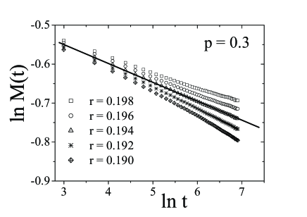
Figure 1: Log-log plots of the order parameter (magnetization) $M(t)$ versus $t$, constructed for $p=0.3$ and different values of $r$. The best linear fitting yields the best estimate for the critical value of the parameter $r$. From the results summarized in Table 1 (see text), we have located the critical point $(p=0.3;r=0.194)$.

For each value of $r$ used in Fig. 1 we calculated the goodness of fit $Q$ for the same time interval $[t_{1},t_{2}]$ and obtained the values shown in Table 1, from which we obtain the critical value $r=0.194$.

Table 1: Values of $Q$ for different values of $r$ obtained from linear fitting of log-log plots of the magnetization $M(t)$ versus $t$.

Time interval	$r$	$Q$
$[50,300]$	$0.190$	$2.31\times 10^{-7}$
$[50,300]$	$0.192$	$0.166$
$[50,600]$	$0.194$	$0.468$
$[50,300]$	$0.196$	$1.04\times 10^{-28}$
$[50,300]$	$0.198$	$1.09\times 10^{-76}$

In order to confirm the critical value obtained in Table 1, we have also calculated the critical value of $r$ for $p=0.3$ by using the effective exponent, which is given by grassberger96

$$\lambda(t)=\dfrac{1}{\Delta t}\log\left(\frac{M(t)}{M(t/\Delta t)}\right).$$ (24)

Such exponent takes into account finite-time corrections (finite-time scaling) and, in the limit $t\rightarrow\infty$, Eq. (24) behaves as grassberger96

$$\lambda(t)=c_{1}+c_{2}/t,$$ (25)

where $c_{1}$ and $c_{2}$ are numerical constants and $\Delta t$ is a fixed time step.

Log-log plots of Eq. (24) are shown in Fig. 2, for $\Delta t=10$, $p=0.3$ and $r=0.190,0.192,0.194,0.196$ and $0.198$. From Fig. 2 it is clear that the asymptotic behavior of $\lambda(t)$ given by Eq. (25) is verified for $r=0.194$, thus confirming the result previously obtained from log-log plots of Eq. (2).

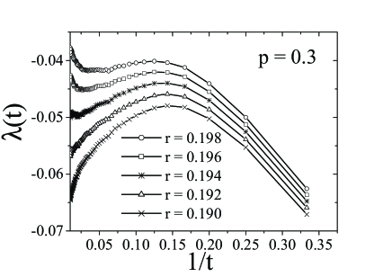
Figure 2: Effective exponent $\lambda(t)$ obtained for $p=0.3$ and different values of $r$. From this graph, we have obtained the critical point $(p=0.3;r=0.194)$ (See text for details).

Before presenting the estimates obtained for the critical exponents $z$ and $\theta_{g}$ in the next subsections, it is important to emphasize here that the Monte Carlo simulations were performed only at the critical point $(p=0.3;r=0.194)$.

IV.2 Critical dynamic exponent $z$

In order to obtain the dynamic critical exponent $z$ we have perfomed short-time Monte Carlo simulations for square lattices $(d=2)$ with linear dimensions $L=160$, $N_{s}=20000$ samples, $N_{b}=5$ sets of samples and 200 MCS. From the definition of the ratio $F_{2}$ given by Eq. (5), we have constructed the log-log plot of $F_{2}(t)$ versus $t$ shown in Fig. 3, obtained from Monte Carlo simulations performed for one set of samples. The straight line depicted in Fig. 3 is in accordance with the linear behavior predicted in the scaling relation of Eq. (5).

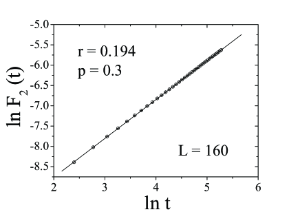
Figure 3: Typical log-log plot of $F_{2}(t)$ versus $t$ (straight line), obtained from short-time Monte Carlo simulations at the critical point $(p=0.3;r=0.194)$.

In Table 2 we summarize the estimates for $z$ obtained from different time intervals $[t_{1},t_{2}]$, together with the corresponding values of $Q$.

Table 2: Dynamic critical exponent $z$ and the corresponding value of $Q$ obtained for different time intervals.

Time interval	$z$	$Q$
$[10,120]$	$2.0853(7)$	$0.2$
$[10,160]$	$2.0856(5)$	$0.49$
$[10,200]$	$2.0869(4)$	$0.54$
$[30,200]$	$2.084(4)$	$0.98$
$[100,200]$	$2.097(8)$	$0.99$

From Table 2, we have obtained the best estimate for the dynamic critical exponent $z=2.097(8)$, once the goodness of fit $Q=0.99$ is maximum at the corresponding time interval. However, such value of $z$ is somewhat smaller than $z=2.17(2)$, which was obtained from the fourth order Binder’s cumulant tome98 . In order to check the value of $z$ obtained in this work, in the next section we obtain the global persistence exponent from the collapse method, which depends on the value of $z$, and directly from Eq. (20), which does not depend on the value of $z$. As we shall see in the following, the results for $\theta_{g}$ obtained from these two approaches are in very good agreement with each other.

IV.3 Critical dynamic exponent $\theta_{g}$

By using Eqs. (21), (22) and (23) given in section III.2, we have performed short-time Monte Carlo simulations in order to apply the collapse method of section III.2 and obtain the dynamic critical exponent $\theta_{g}$. According with the description of the method, the dynamic exponent $z$ is to be known beforehand. Thus, we have used the value $z=2.097$ obtained in the previous section. Monte Carlo runs were made up to 1000 MCS for $N_{s}=40000$ samples in square lattices with linear dimensions 20, 40 and 80. The collapse method was applied for pairs of linear dimensions $(L_{1},L_{2})=(20,40)$ and $(L_{1},L_{2})=(40,80)$, from which we have obtained $\theta_{g}=0.24(2)$ and $\theta_{g}=0.25(2)$, respectively. In Fig. 4 we show the collapse of the curves obtained for $L=40$ and $L=80$ with $\theta_{g}=0.25$.

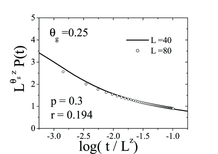
Figure 4: Collapse obtained from the scaling relation Eq. (21), corresponding to square lattices with linear dimensions $(L_{1},L_{2}=40,80)$ and $\theta_{g}=0.25$.

Finally, we have obtained the dynamic exponent $\theta_{g}$ directly from the power law predicted in Eq. (20). To this end, we have performed short-time Monte Carlo simulations to obtain the quantity $P(t)$, from which we have constructed log-log curves of $P(t)$ versus $t$, as depicted in Fig. 5.

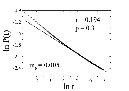
Figure 5: Typical decay of the probability $P(t)$ (straight line in a log-log plot), obtained from short-time Monte Carlo simulations of $N_{s}=40000$ samples with initial state $m_{0}=0.005$.

From Eq. (20), the exponent $\theta_{g}$ was obtained directly from the slope of such curves. Monte Carlo simulations were performed for square lattices with linear dimension $L=80$ and $N_{s}=40000$ samples, where each sample began from the initial state $m_{0}=0.005$. Error bars were estimated from the Monte Carlo runs performed for $N_{b}=5$ sets of samples. In Table 3 we present the results obtained for the exponent $\theta_{g}$ and the corresponding goodness of fit $Q$ for three different time intervals.

Table 3: Dynamic critical exponent $\theta_{g}$ and the corresponding value of $Q$ obtained for different time intervals.

Time interval	$\theta_{g}$	$Q$
$[90,300]$	$0.247(4)$	$0.97$
$[90,400]$	$0.242(3)$	$0.86$
$[100,500]$	$0.238(6)$	$0.95$

From Table 3 above, the best estimate for the global persistence exponent is $\theta_{g}=0.247(4)$, corresponding to $Q=0.97$. This result is in very good agreement with the estimates $\theta_{g}=0.24(2)$ and $\theta_{g}=0.25(2)$ obtained from the collapse method.

V Conclusions

In this work we have revisited the probabilistic cellular automata proposed by Tomé and Drugowich tome96 on the basis of a previous cellular automaton devised by Brass et al. brass94 . From short-time Monte Carlo simulations, we have obtained the dynamic critical exponent $z=2.097(8)$ by using a recent technique that mixes different initial conditions dasilva02 . Such result is slightly smaller than the value $z=2.17(2)$ obtained from the fourth order Binder’s cumulant tome98 .

We have also performed short-time Monte Carlo simulations in order to obtain estimates for the dynamic critical exponent $\theta_{g}$, the global persistence exponent, by using two distinct approaches: The collapse method described by Eqs. (21), (22) and (23), and directly from the power law scaling given by Eq. (20). From the collapse method, by using square lattices with linear dimensions $(L_{1},L_{2})=(20,40)$ and $(L_{1},L_{2})=(40,80)$, we have obtained $\theta_{g}=0.24(2)$ and $\theta_{g}=0.25(2)$, respectively. Directly from Eq. (20) we have obtained $\theta_{g}=0.247(4)$, in very good agreement with the estimates yielded from the collapse method.

References

- (1) M. Bezzi. Modeling evolution and immune system by cellular automata. Riv. Nuovo Cimento, 24(2):1–50, 2001.
- (2) A. Brass, A. J. Bancroft, M. E. Clamp, R. K. Grencis, and K. J. Else. Dynamical and critical behavior of a simple discrete model of the cellular immune system. Phys. Rev. E, 50(2):1589–1593, aug 1994.
- (3) A. Brass, R. K. Grencis, and K. J. Else. A cellular-automata model for helper t-cell subset polarization in chronic and acute infection. J. Theor. Biol., 166(2):189–200, jan 1994.
- (4) R. M. Z. dos Santos and S. Coutinho. Dynamics of HIV infection: A cellular automata approach. Phys. Rev. Lett., 87(16):168102–1–168102–4, oct 2001.
- (5) K. J. Else, G. M. Entwistle, and R. K. Grencis. Correlations between worm burden and markers of TH1 and TH2 cell subset induction in an inbred strain of mouse infected with trichuris-muris. Parasite Immunol., 15(10):595–600, oct 1993.
- (6) T. Tomé and J. R. Drugowich de Felício. Probabilistic cellular automaton describing a biological immune system. Phys. Rev. E, 53(4):3976–3981, apr 1996.
- (7) N. R. S. Ortega, C. F. S. Pinheiro, T. Tomé, and J. R. Drugowich de Felício. Critical behavior of a probabilistic cellular automaton describing a biological system. Phys. Lett. A, 233:93–98, aug 1997.
- (8) G. Grinstein, C. Jayaprakash, and H. Yu. Statistical Mechanics of Probabilistic Cellular Automata. Phys. Rev. Lett., 55(23):2527–2530, dec 1985.
- (9) T. Tomé and J. R. Drugowich de Felício. Short-time dynamics of an irreversible probabilistic cellular automaton. Mod. Phys. Lett. B, 12(21):873–879, sep 1998.
- (10) R. da Silva, N. A. Alves, and J. R. Drugowich de Felício. Mixed initial conditions to estimate the dynamic critical exponent in short-time Monte Carlo simulation. Phys. Lett. A, 298:325–329, apr 2002.
- (11) H. K. Janssen, B. Schaub, and B. Schmittmann. New universal short-time scaling behavior of critical relaxation processes. Z. Phys. B, 73(4):539–549, 1989.
- (12) B. Zheng. Monte Carlo simulations of short-time critical dynamics. Int. J. Mod. Phys. B, 12(14):1419–1484, jun 1998.
- (13) N Alves Jr. and J. R. Drugowich de Felício. Short-time dynamic exponents of an Ising model with competing interactions. Mod. Phys. Lett. B, 17(5–6):209–218, mar 2003.
- (14) E. Arashiro and J. R. Drugowich de Felício. Short-time critical dynamics of the Baxter-Wu model. Phys. Rev. E, 67(4):046123, apr 2003.
- (15) R. da Silva, N. A. Alves, and J. R. Drugowich de Felício. Universality and scaling study of the critical behavior of the two-dimensional Blume-Capel model in short-time dynamics. Phys. Rev. E, 66(2):026130, aug 2002.
- (16) N Alves Jr. and J. R. Drugowich de Felício. Short-time critical dynamics at the Lifshitz point of the ANNNI model. , to be published.
- (17) R. da Silva, J. R. Drugowich de Felício, and R. Dickman. , cond-mat/0404065.
- (18) S. N. Majumdar, A. J. Bray, S. J. Cornell, and C. Sire. Global Persistence Exponent for Nonequilibrium Critical Dynamics. Phys. Rev. Lett., 77(18):3704–3707, oct 1996.
- (19) S. Wolfram. Statistical-Mechanics of Cellular Automata. Rev. Mod. Phys., 55(3):601–644, 1983.
- (20) R. da Silva, N. A. Alves, and J. R. Drugowich de Felício. Global Persistence Exponent of the Two-Dimensional Blume-Capel Model. Phys. Rev. E, 67(5):057102, may 2002.
- (21) P. Grassberger and Y. Zhang. “Self-organized” formulation of standard percolation phenomena. Physica A, 224(1–2):169–179, feb 1996.