Theory of acoustic surface plasmons

Abstract

Recently, a novel low-energy collective excitation has been predicted to exist at metal surfaces where a quasi two-dimensional (2D) surface-state band coexists with the underlying three-dimensional (3D) continuum. Here we present a model in which the screening of a semiinfinite 3D metal is incorporated into the description of electronic excitations in a 2D electron gas through the introduction of an effective 2D dielectric function. Our self-consistent calculations of the dynamical response of the 3D substrate indicate that an acoustic surface plasmon exists for all possible locations of the 2D sheet relative to the metal surface. This low-energy excitation, which exhibits linear dispersion at low wave vectors, is dictated by the nonlocality of the 3D dynamical response providing incomplete screening of the 2D electron-density oscillations.

I introduction

Since the early suggestion of Pinespines1 that low-energy plasmons with sound-like long-wavelength dispersion could be realized in the collective motion of a system of two types of electronic carriers, these modes have spurred over the years a remarkable interest and research activity.tosi

The possibility of having a longitudinal acoustic mode in a metal-insulator-semiconductor (MIS) structure was anticipated by Chaplik.chaplik Chaplik considered a simplified model in which a two-dimensional (2D) electron gas is separated from a semiinfinite three-dimensional (3D) metal. He found that the screening of valence electrons in the metal changes the 2D plasmon energy from its characteristic square-root wave-vector dependence to a linear dispersion, which was also discussed by Gumhaltergum in his study of transient interactions of surface-state electron-hole (e-h) pairs at surfaces.

Nevertheless, acoustic plasmons were only expected to exist for spatially separated plasmas, as pointed out by Das Sarma and Madhukar.sarma The experimental realization of two-dimensionally confined and spatially separated multicomponent structures, such as quantum wells and heterostructures, provided suitable solid-state systems for the observation of acoustic plasmons.olego Acoustic plasma oscillations were then proposed as possible candidates to mediate the attractive interaction leading to the formation of Cooper pairs in high-$T_{c}$ superconductors.ruvalds ; bill

Recently, Silkin et al.silkin have shown that metal surfaces where a partially occupied quasi-2D surface-state band coexists in the same region of space with the underlying 3D continuum support a well-defined acoustic surface plasmon, which could not be explained within the original local model of Chaplik.chaplik This low-energy collective excitation exhibits linear dispersion at low wave vectors, and might therefore affect e-h and phonon dynamics near the Fermi level.note00

In this paper, we present a model in which the screening of a semiinfinite 3D metal is incorporated into the description of electronic excitations in a 2D electron gas through the introduction of an effective 2D dielectric function. We find that the dynamical screening of valence electrons in the metal changes the 2D plasmon energy from its characteristic square-root behaviour to a linear dispersion, not only in the case of a 2D sheet spatially separated from the semiinfinite metal, as anticipated by Chaplik,chaplik but also when the 2D sheet coexists in the same region of space with the underlying metal, as occurs in the real situation of surface states at a metal surface. Furthermore, our results indicate that it is the nonlocality of the 3D dynamical response which allows the formation of 2D electron-density acoustic oscillations at metal surfaces, since these oscillations would otherwise be completely screened by the surrounding 3D substrate.

Unless stated otherwise, atomic units are used throughout, i.e., $e^{2}=\hbar=m_{e}=1$.

II theory

A variety of metal surfaces, such as Be(0001) and the (111) surfaces of the noble metals Cu, Ag, and Au, are known to support a partially occupied band of Shockley surface states with energies near the Fermi level.ingles Since the wavefunction of these states is strongly localized near the surface and decays exponentially into the solid, they can be considered to form a 2D electron gas.

In order to describe the electronic excitations occurring within a surface-state band that is coupled with the underlying continuum of valence electrons in the metal, we consider a model in which surface-state electrons comprise a 2D electron gas at $z=z_{d}$ ($z$ denotes the coordinate normal to the surface), while all other states of the metal comprise a 3D substrate consisting of a fixed uniform positive background (jellium) of density

$$n_{+}(z)=\cases{\bar{n},&$z\leq 0$\cr\cr 0,&elsewere,}$$ (1)

plus a neutralizing inhomogeneous cloud of interacting electrons. The positive-background charge density $\bar{n}$ is often expressed in terms of the 3D Wigner radius $r_{s}^{3D}=(3/4\pi\bar{n})^{1/3}/a_{0}$, $a_{0}=0.529\AA$ being the Bohr radius.

We consider the response of the interacting 2D and 3D electronic subsystems to an external potential $\phi^{ext}({\bf r},\omega)$. According to time-dependent perturbation theory, keeping only terms of first order in the external perturbation, and Fourier transforming in two directions, the electron densities induced in the 2D and 3D subsystems are found to be

$$\delta n_{2D}(z;q,\omega)=\delta(z-z_{d})\,\chi_{2D}(q,\omega)$$ (2)

$$\times \left[\phi^{ext}(z;q,\omega)+\int dz^{\prime}v(z,z^{\prime};q)\delta n_{3D}(z^{\prime};q,\omega)\right]$$ (4)

and

$$\delta n_{3D}(z;q,\omega)=\int dz^{\prime}\,\chi_{3D}(z,z^{\prime};q,\omega)$$ (5)

$$\times \left[\phi^{ext}(z^{\prime};q,\omega)+\int dz^{\prime\prime}v(z^{\prime},z^{\prime\prime};q)\delta n_{2D}(z^{\prime\prime};q,\omega)\right].$$ (7)

Here, $q$ is the magnitude of the 2D wave vector parallel to the surface, $\chi_{2D}(q,\omega)$ and $\chi_{3D}(z,z^{\prime};q,\omega)$ are 2D and 3D interacting density response functions, respectively, $\phi^{ext}(z;q,\omega)$ is the 2D Fourier transform of the external potential $\phi^{ext}({\bf r},\omega)$, and $v(z,z^{\prime};q)$ is the 2D Fourier transform of the bare Coulomb interaction:

$$v(z,z^{\prime};q)=v_{q}\,{\rm e}^{-q\,|z-z^{\prime}|},$$ (8)

with $v_{q}=2\pi/q$.

Combining Eqs. (2) and (5), we find

$$\delta n_{2D}(z;q,\omega)=\delta(z-z_{d})\,\chi_{eff}(q,\omega)\,\tilde{\phi}(z;q,\omega),$$ (9)

where

$$\chi_{eff}(q,\omega)={\chi_{2D}(q,\omega)\over 1-\chi_{2D}(q,\omega)\left[W(z_{d},z_{d};q,\omega)-v_{q}\right]},$$ (10)

$W(z_{d},z_{d};q,\omega)$ being the so-called screened interaction

$$W(z,z^{\prime};q,\omega)=v(z,z^{\prime};q)+\int dz_{1}\int dz_{2}$$ (11)

(12)

$$\times\,v(z,z_{1};q)\,\chi_{3D}(z_{1},z_{2};q,\omega)\,v(z_{2},z^{\prime};q),$$ (13)

and $\tilde{\phi}(z;q,\omega)$ being the 2D Fourier transform of the total potential at $z$ in the absence of the 2D sheet:

$$\tilde{\phi}(z;q,\omega) = \int dz^{\prime\prime}\left[\delta(z-z^{\prime\prime})+\int dz^{\prime}\,v(z,z^{\prime};q)\right.$$ (14)

$$\times \left.\chi_{3D}(z^{\prime},z^{\prime\prime};q,\omega)\right]\phi^{ext}(z^{\prime\prime};q,\omega).$$ (16)

Eq. (9) suggests that the screening of the 3D subsystem can be incorporated into the description of the electron-density response at the 2D electron gas through the introduction of the effective density-response function of Eq. (10), whose poles should correspond to 2D electron-density oscillations.

Alternatively, we can focus on the 2D Fourier transform of the total potential at $z$ in the presence of both 2D and 3D subsystems:

$$\phi(z;q,\omega) = \phi^{ext}(z;q,\omega)+\int dz^{\prime}\,v(z,z^{\prime};q)$$ (17)

$$\times \left[\delta n_{2D}(z^{\prime};q,\omega)+\delta n_{3D}(z^{\prime};q,\omega)\right],$$ (19)

which with the aid of Eqs. (5) and (14) can also be expressed in the following way:

$$\phi(z;q,\omega)=\tilde{\phi}(z;q,\omega)+\int dz^{\prime}W(z,z^{\prime};q,\omega)\,\delta n_{2D}(z^{\prime};q,\omega).$$ (20)

Now we choose $z=z_{d}$, and using Eq. (9) we write

$$\phi(z_{d};q,\omega)=\left[1+W(z_{d},z_{d};q,\omega)\,\chi_{eff}(q,\omega)\right]\,\tilde{\phi}(z_{d};q,\omega),$$ (21)

which allows to introduce the effective inverse 2D dielectric function

$$\epsilon_{eff}^{-1}(q,\omega)=1+W(z_{d},z_{d};q,\omega)\,\chi_{eff}(q,\omega).$$ (22)

Since our aim is to investigate the occurrence of long-wavelength ($q\to 0$) collective excitations, we can rely on the random-phase approximation (RPA),pines2 which is exact in the $q\to 0$ limit. In this approximation, the 2D and 3D interacting density-response functions are obtained as follows

$$\chi_{2D}(q,\omega)={\chi_{2D}^{0}(q,\omega)\over 1-\chi_{2D}^{0}(q,\omega)\,v_{q}}$$ (23)

and

$$\chi_{3D}(z,z^{\prime};q,\omega)=\chi_{3D}^{0}(z,z^{\prime};q,\omega)+\int dz_{1}\int dz_{2}$$ (24)

(25)

$$\times\,\chi_{3D}^{0}(z,z_{1};q,\omega)\,v(z_{1},z_{2};q)\,\chi_{3D}(z_{2},z^{\prime};q,\omega),$$ (26)

where $\chi_{2D}^{0}(q,\omega)$ and $\chi_{3D}^{0}(z,z^{\prime};q,\omega)$ represent their noninteracting counterparts. An explicit expression for the 2D noninteracting density-response function $\chi_{2D}^{0}(q,\omega)$ was reported by Stern.stern In order to derive explicit expressions for the 3D noninteracting density-response function $\chi_{3D}^{0}(z,z^{\prime};q,\omega)$ one needs to rely on simple models, such as the hydrodynamic or infinite-barrier model, but accurate numerical calculations have been carried outeguiluz ; liebsch from the knowledge of the eigenfunctions and eigenvalues of the Kohn-Sham hamiltonian of density-functional theory (DFT).dft

Combining Eqs. (10), (22), and (23), one finds the RPA effective 2D dielectric function

$$\epsilon_{eff}(q,\omega)=1-W(z_{d},z_{d};q,\omega)\,\chi_{2D}^{0}(q,\omega).$$ (27)

The longitudinal modes of the 2D subsystem, or plasmons, are solutions of

$$\epsilon_{eff}(q,\omega)=0.$$ (28)

In the absence of the 3D subsystem, the 3D screened interaction $W(z,z^{\prime};q,\omega)$ reduces to the bare Coulomb interaction $v(z,z^{\prime};q)$, and the solution of Eq. (28) leads at long wavelengths to the well-known square-root wave-vector dependence of the 2D plasmon energystern

$$\omega_{2D}={q_{F}\over\sqrt{m}}\,\sqrt{q},$$ (29)

$q_{F}$ and $m$ being the 2D Fermi momentum and 2D effective mass, respectively. The 2D Fermi velocity is simply $v_{F}=q_{F}/m$.

In the presence of the 3D subsystem, the long-wavelength limit of the effective 2D dielectric function of Eq. (27) is found to have two zeros. One zero corresponds to a high-frequency ($\omega>>v_{F}q$) oscillation in which 2D and 3D electrons oscillate in phase with one another. The other mode corresponds to a low-frequency acoustic oscillation in which both 2D and 3D electrons oscillate out of phase.

At high frequencies, where $\omega>>v_{F}q$, the long-wavelength limit of the 2D density-response function $\chi_{2D}^{0}(q,\omega)$ is known to be

$$\lim_{q\to 0}\chi_{2D}^{0}(q,\omega>>v_{F}q)={1\over v_{q}}\,{\omega_{2D}^{2}\over\omega^{2}}.$$ (30)

On the other hand, when the 2D sheet is located either far inside or far outside the metal surface, the long-wavelength limit of the 3D screened interaction $W(z_{d},z_{d};q,\omega)$ takes the form

$$\lim_{q\to 0}W(z_{d},z_{d};q,\omega>>v_{F}q)=v_{q}\,{\omega^{2}\over\omega^{2}-\omega_{p,s}^{2}},$$ (31)

where $\omega_{p,s}$ represents either the bulk-plasmon frequency $\omega_{p}=\sqrt{4\,\pi\,\bar{n}}$ or the conventional surface-plasmon energy $\omega_{s}=\omega_{p}/\sqrt{2}$,ritchie depending on whether the 2D sheet is located inside or outside the solid. Introduction of Eqs. (30) and (31) into Eqs. (27) and (28) yields a high-frequency mode at

$$\omega^{2}=\omega_{p,s}^{2}+\omega_{2D}^{2}.$$ (32)

At low frequencies, we seek for an acoustic 2D plasmon energy that in the long-wavelength limit takes the form

$$\omega=\alpha\,v_{F}\,q.$$ (33)

A careful analysis of the 2D density-response function $\chi_{2D}^{0}(q,\omega)$ and the 3D screened interaction $W(z_{d},z_{d};q,\omega)$ shows that at $\omega=\alpha\,v_{F}\,q$ the long-wavelength limits of these quantities take the form

$$\lim_{q\to 0}\chi_{2D}^{0}(q,\alpha v_{F}q)={1\over\pi}\left[{\alpha\over\sqrt{\alpha^{2}-1}}-1\right]$$ (34)

and

$$\lim_{q\to 0}W(z_{d},z_{d};q,\alpha v_{F}q)=I(z_{d}).$$ (35)

An inspection of Eqs. (27), (34), and (35) indicates that for a low-energy acoustic oscillation to occur the quantity $I(z_{d})$ must be different from zero. In that case, the long-wavelength limit of the effective 2D dielectric function of Eq. (27) has indeed a zero corresponding to a low-frequency oscillation of energy given by Eq. (33) with

$$\alpha=\sqrt{1+{\left[I(z_{d})\right]^{2}\over\pi\left[\pi+2\,I(z_{d})\right]}}.$$ (36)

In the following, we investigate the impact of the 3D screening on the actual wave-vector dependence of the low-energy 2D collective excitation. We first consider the two limiting cases in which the 2D sheet is located far inside and far outside the metal surface, and we then carry out self-consistent calculations of the 3D screened interaction $W(z,z^{\prime};q,\omega)$, which will allow us to obtain plasmon dispersions for arbitrary locations of the 2D sheet.

II.1 2D sheet far inside the metal surface

In the case of a 2D sheet that is located far inside the metal surface, the 3D subsystem can safely be assumed to exhibit translational invariance in all directions, i.e., the screened interaction $W(z_{d},z_{d};q,\omega)$ entering Eq. (27) can be easily obtained from the knowledge of the interacting density-response function $\chi_{3D}(k,\omega)$ of a uniform 3D electron gas, as follows

$$W(z_{d},z_{d};q,\omega)=2\int{dq_{z}\over k^{2}}\,\epsilon_{3D}^{-1}(k,\omega),$$ (37)

where $k=\sqrt{q^{2}+q_{z}^{2}}$ is the magnitude of a 3D wave vector and $\epsilon_{3D}^{-1}(k,\omega)$ is the inverse dielectric function of a uniform 3D electron gas:

$$\epsilon_{3D}^{-1}(k,\omega)=1+{4\pi\over k^{2}}\,\chi_{3D}(k,\omega).$$ (38)

In the RPA,

$$\epsilon_{3D}(k,\omega)=1-{4\pi\over k^{2}}\,\chi_{3D}^{0}(k,\omega),$$ (39)

$\chi_{3D}^{0}(k,\omega)$ being the noninteracting density-response function first obtained by Lindhard.lindhard

II.1.1 Local 3D response

If one characterizes the 3D uniform electron gas by a local dielectric function $\epsilon_{3D}(\omega)$, then Eq. (37) yields

$$W^{local}(z_{d},z_{d};q,\omega)=v_{q}\,\epsilon_{3D}^{-1}(\omega).$$ (40)

In a 3D gas of free electrons, $\epsilon_{3D}(\omega)$ takes the Drude form

$$\epsilon_{3D}(\omega)=1-{\omega_{p}^{2}\over\omega^{2}},$$ (41)

which yields

$$\lim_{q\to 0}W^{local}(z_{d},z_{d};q,\alpha v_{F}q)=0.$$ (42)

This means that in a local picture of the 3D response the characteristic collective oscillations of the 2D electron gas would be completely screened by the sorrounding 3D substrate and no low-energy acoustic mode would exist.note01

II.1.2 Hydrodynamic 3D response

Dispersion effects of the 3D subsystem can be incorporated approximately in a hydrodynamic model. In this approximation, the dielectric function of a 3D uniform electron gas is found to belindhard

$$\epsilon_{3D}(k,\omega)=1-{\omega_{p}^{2}\over\omega^{2}-\beta^{2}\,k^{2}},$$ (43)

where $\beta=\sqrt{1/3}\,k_{F}$ represents the speed of propagation of hydrodynamic disturbances in the electron system,note0 and $k_{F}$ is the 3D Fermi momentum.

Introducing Eq. (43) into Eq. (37), one finds

$$\lim_{q\to 0}W(z_{d},z_{d};q,\alpha v_{F}q)=2\pi\beta/\omega_{p},$$ (44)

which yields the following simple expression for the acoustic coefficient of Eq. (36):

$$\alpha=\sqrt{1+{4\beta^{2}/\omega_{p}^{2}\over 1+4\beta/\omega_{p}}}.$$ (45)

II.1.3 Full 3D response

We have carried out numerical calculations of the RPA effective dielectric function of Eq. (27), by using the full $\chi_{2D}^{0}(q,\omega)$ and $\chi_{3D}^{0}(k,\omega)$ density-response functions, and choosing the electron-density parameters $r_{s}^{2D}=3.14$ and $r_{s}^{3D}=1.87$ corresponding to the (0001) surface of Be.note1

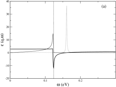
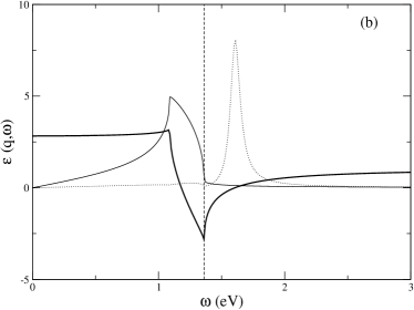
Figure 1: Effective dielectric function of a 2D sheet that is located far inside the metal surface, as obtained from Eq. (27) with (a) $q=0.01$ and (b) $q=0.1$. The real and the imaginary parts of $\epsilon_{eff}(q,\omega)$ are represented by thick and thin solid lines, respectively. The dotted line represents the effective 2D energy-loss function ${\rm Im}\left[-\epsilon_{eff}^{-1}(q,\omega)\right]$. The vertical dashed line represents the upper edge $\omega_{u}=v_{F}q+q^{2}/(2m)$ of the 2D e-h pair continuum, where 2D e-h pairs can be excited. 2D and 3D electron densities have been taken to be those corresponding to the Wigner radii $r_{s}^{2D}=3.14$ and $r_{s}^{3D}=1.87$, respectively. The 2D effective mass has been taken to be $m=1$.

The results we have obtained with $q=0.01a_{0}^{-1}$ and $q=0.1a_{0}^{-1}$ are displayed in Figs. 1a and 1b, respectively. We observe that at energies below the upper edge $\omega_{u}=v_{F}q+q^{2}/(2m)$ (vertical dashed line) of the 2D e-h pair continuum (where 2D e-h pairs can be excited) the real part of the effective dielectric function is nearly constant and the imaginary part is large, as would occur in the absence of the 3D susbtrate. At energies above $\omega_{u}$, momentum and energy conservation prevents 2D e-h pairs from being produced, and ${\rm Im}\,\epsilon_{eff}(q,\omega)$ is very small.

Collective excitations are related to a zero of ${\rm Re}\,\epsilon_{eff}(q,\omega)$ in a region where ${\rm Im}\,\epsilon_{eff}(q,\omega)$ is small and lead, therefore, to a maximum in the energy-loss function ${\rm Im}[-\epsilon_{eff}^{-1}(q,\omega)]$.loss In the absence of the 3D substrate, a 2D plasmon would occur at $\omega_{2D}=1.22\,{\rm eV}$ for $q=0.01a_{0}^{-1}$ and $\omega_{2D}=3.99\,{\rm eV}$ for $q=0.1a_{0}^{-1}$. However, Fig. 1 shows that in the presence of the 3D substrate a well-defined low-energy acoustic plasmon occurs, the sound velocity being just over the 2D Fermi velocity $v_{F}$. The small width of the plasmon peak is entirely due to plasmon decay into e-h pairs of the 3D substrate.

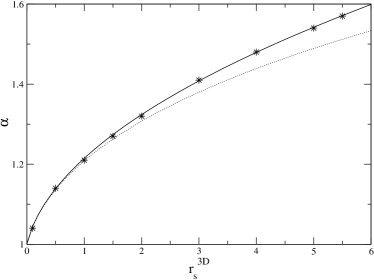
Figure 2: Stars represent the $\alpha$ coefficient of the acoustic-plasmon energy $\omega=\alpha\,v_{F}\,q$ versus the 3D Wigner radius, as obtained from Eq. (28) in the long-wavelength limit. These results are found to be insensitive to the 2D Wigner radius $r_{s}^{2D}$. The solid line represents the prediction of Eq. (36), as obtained with the full RPA value of $I(z_{d}\to-\infty)$. The dotted line represents the hydrodynamic prediction of Eq. (45).

We have carried out calculations of the effective 2D dielectric function of Eq. (27) for a variety of 2D and 3D electron densities, and we have found that a well-defined acoustic plasmon of energy $\omega=\alpha\,v_{F}\,q$ is always present for 2D wave vectors up to a maximum value of $q\sim q_{F}$ where the acoustic-plasmon dispersion merges with $\omega_{u}$. The coefficient $\alpha$ that we have obtained from the zeros in Eq. (28) is represented by stars in Fig. 2 versus the 3D Wigner radius $r_{s}^{3D}$, together with the prediction of Eq. (36) as obtained with the computed RPA value of $I(z_{d}\to-\infty)$ (solid line) and the hydrodynamic prediction of Eq. (45) (dotted line). Fig. 2 shows that Eq. (45) is a good representation of the linear dispersion of this low-energy plasmon, especially at the highest 3D electron densities. Fig. 2 also shows that for low electron densities the hydrodynamic prediction is too small, which is due to the fact that at low densities the long-wavelength limit of the 3D screened interaction is underestimated in this approximation.

II.2 2D sheet far outside the metal surface

In the case of a 2D sheet that is located far outside the metal surface, where the 3D electron density is negligible, the 3D screened interaction of Eq. (11) at $z=z^{\prime}=z_{d}$ takes the form

$$W(z_{d},z_{d};q,\omega)=v_{q}\left[1-{\rm e}^{-2\,q\,z_{d}}\,g(q,\omega)\right],$$ (46)

where $g(q,\omega)$ is the so-called surface-response function of the 3D subsystem

$$g(q,\omega)=-v_{q}\int dz_{1}\int dz_{2}\,{\rm e}^{q\,(z_{1}+z_{2})}\,\chi_{3D}(z_{1},z_{2};q,\omega).$$ (47)

II.2.1 Local 3D response

In the simplest possible model of a metal surface, one characterizes the 3D substrate at $z\leq 0$ by a local dielectric function which jumps discontinuously at the surface from $\epsilon_{3D}(\omega)$ inside the metal ($z\leq 0$) to zero outside ($z>0$). Witin this model,liebsch2

$$g^{local}(q,\omega)={\epsilon_{3D}(\omega)-1\over\epsilon_{3D}(\omega)+1},$$ (48)

which is precisely the long-wavelength limit of the actual surface-response function.

At low frequencies, where $\epsilon_{3D}(\omega)$ is large [see Eq. (41)] and $g^{local}(q,\omega)\to 1$, Eq. (46) yields

$$\lim_{q\to 0}W^{local}(z_{d},z_{d};q,\alpha v_{F}q)=4\,\pi\,z_{d}.$$ (49)

Introducing Eq. (49) into Eq. (36), one finds

$$\alpha=\sqrt{1+{16\,z_{d}^{2}\over 1+8\,z_{d}}}.$$ (50)

For large values of the distance $z_{d}$ between the 2D sheet and the metal surface, one can write

$$\alpha\approx\sqrt{2z_{d}},$$ (51)

which is the result first obtained by Chaplikchaplik by using the Drude-like 2D density-response function of Eq. (30).

II.2.2 Nonlocal 3D response

An inspection of Eq. (46) shows that the long-wavelength limit of the screened interaction $W(z_{d},z_{d};q,\omega)$ is dictated not only by the local ($q=0$) surface-response function $g^{local}(q,\omega)$ but also by the leading correction in $q$ of the actual nonlocal $g(q,\omega)$. Feibelman showed that up to first order in an expansion in powers of $q$, the surface-response function of a jellium surface can be written asfeibelman

$$g(q,\omega)={\epsilon_{3D}(\omega)-1\over\epsilon_{3D}(\omega)+1}\left[1+2qd_{\perp}(\omega){\epsilon_{3D}(\omega)\over\epsilon_{3D}(\omega)+1}\right]+O(q^{2}),$$ (52)

which at low frequencies yields

$$g(q,\omega)\approx 1+2\,q\,d_{\perp}(0).$$ (53)

The frequency-dependent $d_{\perp}(\omega)$ function occurring in Eq. (52) represents the centroid of the induced 3D charge density, which in the static limit ($\omega=0$) reduces to the image plane of an external point charge.

Using Eq. (53), we find the actual long-wavelength limit of Eq. (46):

$$\lim_{q\to 0}W(z_{d},z_{d};q,\alpha v_{F}q)=4\,\pi\,\left[z_{d}-d_{\perp}(0)\right],$$ (54)

which combined with Eq. (36) yields

$$\alpha=\sqrt{1+{16\,\left[z_{d}-d_{\perp}(0)\right]^{2}\over 1+8\,\left[z_{d}-d_{\perp}(0)\right]}}.$$ (55)

This shows that the acoustic-plasmon sound velocity derived from the local model [see Eq. (50)] remains unchanged, as long as $z_{d}$ is replaced by the coordinate of the 2D sheet relative to the position of the image plane.

II.2.3 Full 3D response

In order to compute the full RPA surface-response function of Eq. (47), we follow the method described in Ref. eguiluz, for a jellium slab. We first assume that the 3D electron density vanishes at a distance $z_{0}$ from either jellium edge,z0 and compute the noninteracting density-response function $\chi_{3D}^{0}(z,z^{\prime};q,\omega)$ from the knowledge of the self-consistent Kohn-Sham wavefunctions and energies of DFT,dft which we obtain in the local-density approximation (LDA).lda We then introduce a double-cosine Fourier representation for both the noninteracting and the interacting density-response functions, and find explicit expressions for the surface-response function in terms of the Fourier coefficients of the density-response function.aran To ensure that our slab calculations are a faithful representation of the actual surface-response function of a semiinfinite 3D system, we follow the extrapolation procedure described in Ref. pitarke, .

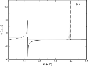
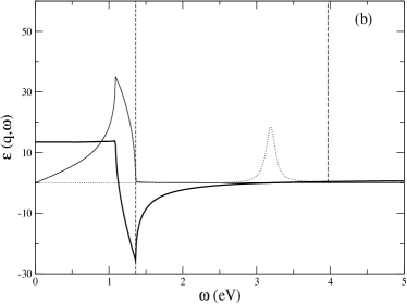
Figure 3: As in Fig. 1, but now for a 2D sheet that is located at one 3D Fermi wavelength outside the metal surface ($z_{d}=\lambda_{F}$). The long-dashed vertical lines here represent the plasmon-energy $\omega=\alpha\,v_{F}\,q$ predicted by Eq. (55) with $d_{\perp}=0.2\,\lambda_{F}$. For real frequencies, a 2D sheet that is located at $z_{d}=\lambda_{F}$ exhibits a plasmon peak that at $q=0.01\,a_{0}^{-1}$ is extremely sharp (as $z_{d}\to\infty$ the plasmon peak becomes a delta function); hence, in the calculations presented in this figure we have replaced the energy $\omega$ by a complex quantity $\omega+i\eta$ with (a) $\eta=0.05\,{\rm eV}$ for $q=0.01\,a_{0}^{-1}$ and (b) $\eta=0$ for $q=0.1\,a_{0}^{-1}$.

We have carried out numerical calculations of the effective dielectric function of Eq. (27), by using the full 2D noninteracting density-response function, $\chi_{2D}^{0}(q,\omega)$, and the self-consistent RPA surface-response function, $g(q,\omega)$, with electron-density parameters $r_{s}^{2D}=3.14$ and $r_{s}^{3D}=1.87$ corresponding to Be(0001).

The results we have obtained for a 2D sheet located at $z_{d}=\lambda_{F}$ are displayed in Figs. 3a (with $q=0.01a_{0}^{-1}$) and 3b (with $q=0.1a_{0}^{-1}$), $\lambda_{F}=2\pi/k_{F}$ being the 3D Fermi wavelength. Fig. 3 clearly shows that in the presence of the 3D substrate a well-defined low-energy acoustic plasmon occurs, the sound velocity being close to that predicted by Eq. (55) with $d_{\perp}(0)=0.2\,\lambda_{F}$ (vertical long-dashed lines). The actual plasmon energy is smaller than predicted by Eq. (55), especially at the shortest wavelengths ($q=0.1a_{0}^{-1}$), simply due to the bending of the plasmon dispersion as a function of $q$ (see Fig. 7 below).

II.3 2D sheet at an arbitrary location

II.3.1 Hydrodynamic 3D response

An explicit expression for the screened interaction $W(z,z^{\prime};q,\omega)$ of Eq. (11) can be obtained in a hydrodynamic model in which the 3D electron density is assumed to change abruptly at the surface from $\bar{n}$ inside the metal to zero outside. After writing and linearizing the basic hydrodynamic equations, i.e., the continuity and the Bernouilli equation, we find

$$\lim_{q\to 0}W(z_{d},z_{d};q,\alpha v_{F}q)=\cases{{2\pi\beta\over\omega_{p}}\left(1-{\rm e}^{2z_{d}\omega_{p}/\beta}\right)&$z_{d}\leq 0$\cr\cr 4\,\pi\,z_{d}&$z_{d}>0$},$$ (56)

which combined with Eq. (36) yields an explicit expression for the acoustic coefficient $\alpha$. We note that in a local description of the electronic response of the solid surface ($\beta=0$) the 3D screened interaction $W(z_{d},z_{d};q,\alpha v_{F}q)$ is zero inside the solid ($z_{d}\leq 0$) and $4\,\pi\,z_{d}$ outside ($z_{d}>0$). This shows that in the 2D long-wavelength limit ($q\to 0$) the nonlocality of the 3D response is only present inside the solid ($z_{d}\leq 0$), where finite values of the 3D momentum $k$ are possible.

Alternatively, the screened interaction $W(z,z^{\prime};q,\omega)$ can be obtained within a specular-reflection model (SRM)ritchie2 or, equivalently, a classical infinite-barrier model (CIBM)griffin ; nazarov of the surface, which have the virtue of describing the 3D screened interaction in terms of the bulk dielectric function $\epsilon_{3D}(k,\omega)$ of a 3D uniform (and infinite) electron gas (see Appendix A). If this bulk dielectric function is chosen to be the hydrodynamic dielectric function of Eq. (43), then these models yield Eq. (56). A more accurate description of the bulk dielectric function $\epsilon_{3D}(k,\omega)$ yields a result that still coincides with that of Eq. (56) outside the surface ($z_{d}>0$), though small differences may arise at $z_{d}<0$.

When the 2D sheet is located far inside the metal ($z_{d}<<0$), Eq. (56) yields the hydrodynamic asymptotic behaviour dictated by Eq. (44), and the SRM combined with the RPA bulk dielectric function yields the correct RPA asymptotic behaviour. However, these hydrodynamic and specular-reflection models, which are both based on the assumption that the 3D electron density drops abruptly to zero at the surface, fail to reproduce the correct asymptotic behaviour outside the surface [see Eq. (54)]. This is due to the fact that the leading correction in $q$ of the surface-response function $g(q,\omega)$ is governed by the spill out of the electron density into the vacuum, which is not present in these models.

II.3.2 Full 3D response

For an arbitrary location of the 2D sheet we need to compute the full screened interaction $W(z_{d},z_{d};q,\omega)$ of Eq. (11). To calculate this quantity we consider a jellium slab, as we did to obtain the surface-response function $g(q,\omega)$, and we find explicit expressions in terms of the Fourier coefficients of the interacting density-response function,aran which we compute in the RPA [see Eq. (24)] from the knowledge of the LDA eigenvalues and eigenfunctions of the Kohn-Sham hamiltonian of DFT.

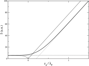
Figure 4: Long-wavelength limit $I(z_{d})$ of the screened interaction $W(z_{d},z_{d};q,\alpha v_{F}q)$. The thick solid line represents the full self-consistent RPA calculation. The results obtained from Eq. (54) with $d_{\perp}(0)=0.2\,\lambda_{F}$ and from Eq. (56) are represented by dotted and thin solid lines, respectively. The horizontal dashed line represents the result obtained from the RPA bulk screened interaction of Eq. (37). The 3D Wigner radius has been taken to be $r_{s}^{3D}=1.87$.

In Fig. 4, the long-wavelength limit $I(z_{d})$ of the screened interaction $W(z_{d},z_{d};q,\alpha v_{F}q)$ [see Eq. (35)] is displayed versus $z_{d}$, as obtained with $r_{s}^{3D}=1.87$ from our full self-consistent RPA calculations (thick solid line) and from the hydrodynamic Eq. (56) (thin solid line). Far inside the solid, our full calculation is close to the hydrodynamic prediction (see also Fig. 2) and coincides with the result one obtains from the bulk screened interaction of Eq. (37) (horizontal dashed line). Near the surface, our full calculation considerably deviates from the hydrodynamic prediction and converges far outside the solid with the asymptotic curve dictated by Eq. (54) with $d_{\perp}(0)=0.2\,\lambda_{F}$ (dotted line).notenew

At this point, it is interesting to note that within a local picture of the 3D response the long-wavelength $I(z_{d})$ screened interaction would be zero for all locations of the 2D sheet inside the metal ($z_{d}\leq 0$), showing that the screening of 2D electron-density oscillations would be complete and no acoustic surface plasmon would occur. It is precisely the nonlocality of the 3D response (finite values of the 3D momentum $k$ are still present in the 2D long-wavelength limit) which provides incomplete screening and allows, therefore, the formation of acoustic surface plasmons in the interior of the solid. We also note that within a simple nonlocal picture of the 3D response, such as the hydrodynamic and specular-reflection models described above, the screening of 2D electron-density oscillations would still be complete at the jellium edge ($z_{d}=0$). Hence, in the real situation where the 2D surface-state band is located very near the jellium edge the occurence of acoustic surface plasmons is originated by a combination of the nonlocality of the 3D response and the spill out of the 3D electron density into the vacuum.

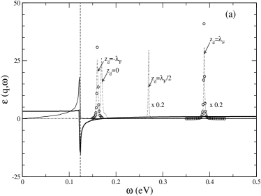
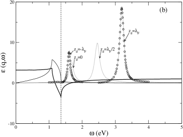
Figure 5: As in Fig. 1, but now for a 2D sheet that is located at the jellium edge ($z_{d}=0$). Also shown is the effective 2D energy-loss function ${\rm Im}\left[-\epsilon_{eff}^{-1}(q,\omega)\right]$ for $z_{d}=-\lambda_{F}$, $z_{d}=\lambda_{F}/2$, and $z_{d}=\lambda_{F}$ (dotted lines). The open circles represent the effective 2D energy-loss function ${\rm Im}\left[-\epsilon_{eff}^{-1}(q,\omega)\right]$ obtained from the limiting Eq. (37) appropriate for a 2D sheet far inside the metal and from the limiting Eq. (46) with $z_{d}=\lambda_{F}$ appropriate for a 2D sheet far outside the metal. These calculations are found to coincide with the full calculations for $z_{d}=-\lambda_{F}$ and $z_{d}=\lambda_{F}$, respectively. As in Fig. 3(a), the calculations presented here for $z_{d}=\lambda_{F}$ and $q=0.01\,a_{0}^{-1}$ have been carried out by replacing the energy $\omega$ by a complex quantity $\omega+i\eta$ with $\eta=0.05\,{\rm eV}$. All remaining calculations have been carried out for real frequencies, i.e., with $\eta=0$.

Figs. 5a and 5b exhibit the results we have obtained for the effective dielectric function of Eq. (27) [with $q=0.01\,a_{0}^{-1}$ (Fig. 5a) and $q=0.1\,a_{0}^{-1}$ (Fig. 5b)] by using the full 2D noninteracting density-response function, $\chi_{2D}^{0}(q,\omega)$, and the self-consistent RPA screened interaction, $W(z_{d},z_{d};q,\omega)$, with electron-density parameters $r_{s}^{2D}=3.14$ and $r_{s}^{3D}=1.87$ corresponding to Be(0001). In these figures the 2D sheet has been taken to be located at $z_{d}=0$, as approximately occurs with the quasi-2D surface-state band in Be(0001). For comparison, also shown in these figures are the results we have obtained for the energy-loss function when the 2D sheet is located inside the metal at $z_{d}=-\lambda_{F}$ and outside the metal at $z_{d}=\lambda_{F}/2$ and $z_{d}=\lambda_{F}$.

An inspection of Fig. 5 shows that (i) the results we have obtained for $z_{d}=-\lambda_{F}$ and $z_{d}=\lambda_{F}$ are exactly reproduced by the limiting Eqs. (37) and (46) appropriate for a 2D sheet far inside and far outside the metal surface, respectively; and (ii) in the actual situation where the 2D surface-state band is located very near the jellium positive background edge ($z_{d}=0$), a well-defined low-energy acoustic plasmon occurs, the sound velocity being very close to the limiting case of a 2D sheet far inside the metal surface and being, therefore, just above $\omega_{u}$. This is in agreement with the recent prediction that in a real metal surface where a partially occupied quasi-2D surface-state band coexists in the same region of space with the underlying 3D continuum an acoustic surface plasmon should occur at energies just above the upper edge of the 2D e-h pair continuum.silkin

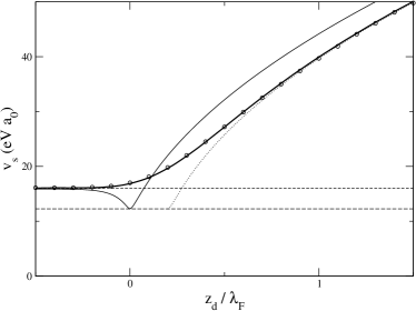
Figure 6: The open circles represent the sound velocity $v_{s}$ ($\omega=v_{s}\,q$) of the low-energy acoustic plasmon that is visible in Fig. 5 versus the location $z_{d}$ of the 2D sheet with respect to the jellium edge. The horizontal short-dashed line represents the result we have obtained from the limiting Eq. (37) appropriate for a 2D sheet far inside the metal. The dotted line represents the result we have obtained from the limiting Eq. (55) with $d_{\perp}=0.2\,\lambda_{F}$, which is appropriate for a 2D sheet far outside the metal. The long-wavelength limit $v_{F}$ of the upper edge $\omega_{u}/q$ of the 2D e-h pair continuum is represented by an horizonal long-dashed line. The thick and thin solid lines represent the results obtained from Eq. (36) by using the actual RPA $I(z_{d})$ and the hydrodynamic Eq. (56), respectively. 2D and 3D electron densities have been taken to be those corresponding to the Wigner radii $r_{s}^{2D}=3.14$ and $r_{s}^{3D}=1.87$, respectively. The 2D effective mass has been taken to be $m=1$.

The sound velocity $v_{s}$ ($\omega=v_{s}\,q$) of the acoustic plasmon that is visible in Fig. 5 is displayed in Fig. 6 versus the location $z_{d}$ of the 2D sheet relative to the jellium edge, as obtained from our full RPA self-consistent calculation of the effective 2D dielectric function of Eq. (27) (open circles), together with the sound velocity $v_{s}=\alpha\,v_{F}$ obtained from Eq. (55) with $d_{\perp}(0)=0.2\,\lambda_{F}$ (dotted line). When the 2D sheet is located inside the metal surface, the sound velocity nicely converges with the RPA bulk calculation from Eq. (37) (horizontal short-dashed line). When the 2D sheet is located outside the metal surface, the sound velocity converges with the limiting value $\alpha\,v_{F}$ obtained from Eq. (55) and $d_{\perp}(0)=0.2\,\lambda_{F}$. For comparison, also shown in this figure is the result we have obtained from Eq. (36) by using the actual RPA $I(z_{d})$ screened interaction (thick solid line) and from the hydrodynamic Eq. (56). These calculations clearly show that Eq. (36) accurately reproduces the dispersion of acoustic surface plasmons, as long as the long-wavelength limit $I(z_{d})$ of the screened interaction is described self-consistently with full inclusion of the electronic selvage structure at the surface.

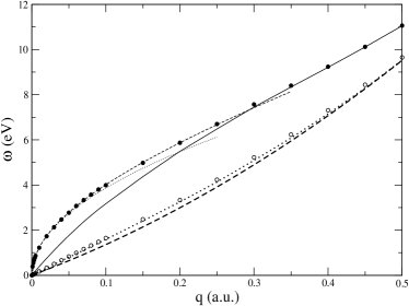
Figure 7: Dispersion of the acoustic plasmon occurring in a 2D sheet that is taken to be located far inside the solid (thick dotted line), at $z_{d}=0$ (open circles), at $z_{d}=\lambda_{F}$ (solid line), and infinitely far outside the metal (solid circles). The thick dashed line represents the upper edge $\omega_{u}=v_{F}q+q^{2}/(2m)$ of the 2D e-h pair continuum. The thin dotted line represents the 2D plasmon energy $\omega_{2D}$ dictated by Eq. (29), which is accurate at long wavelengths ($q\to 0$). The thin dashed line represents the 2D plasmon energy $\sqrt{\omega_{2D}^{2}+3v_{F}^{2}q^{2}/4}$ that is obtained after an expansion of $\chi_{2D}^{0}(q,\omega)$ in powers of $v_{F}q/\omega$. 2D and 3D electron densities have been taken to be those corresponding to the Wigner radii $r_{s}^{2D}=3.14$ and $r_{s}^{3D}=1.87$, respectively. The 2D effective mass has been taken to be $m=1$.

The sound velocity of Fig. 6 (open circles) has been obtained from the effective 2D dielectric function at very low 2D momenta, where the energy of the acoustic plasmon is linear in $q$. The behaviour of this plasmon energy as a function of the 2D momentum $q$ is displayed in Fig. 7, with the 2D sheet chosen to be located far inside the solid (thick dotted line), at $z_{d}=0$ (open circles), at $z_{d}=\lambda_{F}$ (solid line), and infinitely far outside the solid (solid circles). The upper edge of the 2D e-h pair continuum is represented by a thick dashed line, showing that in the real situation where the 2D sheet is located near the jellium edge the energy of the acoustic surface plasmon (open circles) is just outside the 2D e-h pair continuum for all momenta under study.

III Summary and Conclusions

The partially occupied band of Shockley surface states in a variety of metal surfaces is known to form a quasi-2D electron gas that is immersed in a semiinfinite 3D gas of valence electrons. In order to describe the impact of the dynamical screening of the semi-infinite 3D continuum on the electronic excitations at the 2D electron gas of Shockley surface states, we have presented a model in which the dynamical screening of 3D valence electrons is incorporated through the introduction of an effective 2D dielectric function.

We have considered the two limiting cases in which the 2D sheet is located far inside and far outside the metal surface. In both cases, the dynamical screening of the valence electrons in the metal is found to change the 2D plasmon energy from its characteristic square-root behaviour to a linear dispersion, the sound velocity being proportional to the Fermi momentum of the 2D gas. As this collective oscillation occurs in a region of 2D momentum space where 2D e-h pairs cannot be produced, this is a well-defined acoustic plasmon. The finite width of the plasmon peak is due to a small probability for the plasmon to decay into e-h pairs of the 3D substrate.

We have shown explicitly that when the 2D sheet coexists in the same region of space with the underlying 3D continuum the origin of acoustic surface plasmons, which have been overlooked over the years, is dictated by a combination of the nonlocality of the 3D response and the spill out of the 3D electron density into the vacuum, both providing incomplete screening of the 2D electron-density oscillations.

We have carried out self-consistent DFT calculations of the dynamical density-response function of the 3D system of valence electrons, and we have found that a well-defined acoustic plasmon exists for all possible locations of the 2D sheet relative to the metal surface. The energy dispersion of this acoustic surface plasmon is slightly higher than the energy of the collective excitation that has recently been predicted to exist at real metal surfaces where a quasi-2D surface-state band coexists with the underlying 3D continuum.silkin Small differences between the plasmon energies obtained here and those reported previouslysilkin are due to the absence in the present model of transitions between 2D and 3D states.silkin2

Appendix A Specular-reflection model of the 3D response

Either by assuming that electrons are specularly reflected at the surface (SRM)ritchie2 or by invoking the so-called classical infinite-barrier model (CIBM) of a jellium surface,griffin ; nazarov one finds

$$W(z_{d},z_{d};q,\omega)=v_{q}\,\cases{1-{\rm e}^{-2qz_{d}}\left[1-\epsilon_{s}(0;\omega)\right]/\left[1+\epsilon_{s}(0;\omega)\right],&$z_{d}\geq 0$\cr\cr\epsilon_{s}(0;q,\omega)+\epsilon_{s}(2z_{d};q,\omega)-2\epsilon_{s}^{2}(z_{d};q,\omega)/\left[\epsilon_{s}(0;q,\omega)+1\right],&elsewhere},$$ (57)

where $k=\sqrt{q^{2}+q_{z}^{2}}$ is a 3D momentum, and

$$\epsilon_{s}(z;q,\omega)={q\over\pi}\int_{-\infty}^{+\infty}{dq_{z}\over k^{2}}\,{\rm e}^{iq_{z}z}\,\epsilon_{3D}^{-1}(k,\omega),$$ (58)

$\epsilon_{3D}(q,\omega)$ being the dielectric function of a uniform (and infinite) 3D electron gas.

If the 3D dielectric function $\epsilon_{3D}(q,\omega)$ is chosen to be the hydrodynamic dielectric function of Eq. (43), then one finds

$$\epsilon_{s}(z;q,\omega)={1\over\omega^{2}-\omega_{p}^{2}}\left[\omega^{2}-{\beta\omega_{p}^{2}q\over\sqrt{\beta^{2}q^{2}+\omega_{p}^{2}-\omega^{2}}}\right]\,e^{-q|z_{d}|},$$ (59)

which in combination with Eq. (57) yields Eq. (56).

References

- (1) D. Pines, Can. J. Phys. 34, 1379 (1956).
- (2) See, e.g., N. H. March and M. P. Tosi, Adv. Phys. 44, 299 (1995).
- (3) A. V. Chaplik, Zh. Eksp. Teor. Fiz. 62, 746 (1972) [Sov. Phys. JETP 35, 395 (1972)].
- (4) B. Gumhalter, Surf. Sci. 518, 81 (2002).
- (5) S. Das Sarma and A. Madhukar, Phys. Rev. B 23, 805 (1981).
- (6) D. Olego A. Pinczuk, A. C. Gossard, and W. Wiegmann, Phys. Rev. B 25, 7867 (1982).
- (7) J. Ruvalds, Phys. Rev. B 35, 8869 (1987); Nature 328, 299 (1987).
- (8) A. Bill, H. Morawitz, and V. Z. Kresin, Phys. Rev. B 66, 100501 (2002).
- (9) V. M. Silkin, A. García-Lekue, J. M. Pitarke, E. V. Chulkov, E. Zaremba, and P. M. Echenique, Europhys. Lett. 66, 260 (2004).
- (10) The sound velocity of this acoustic mode is, however, close to the Fermi velocity of the 2D surface-state band, which is typically a few orders of magnitude larger than the sound velocity of acoustic phonons in metals.
- (11) J. E. Inglesfield, Rep. Prog. Phys. 45, 223 (1982).
- (12) D. Pines and P. Nozieres, The theory of quantum liquids (Addison-Wesley, New York, 1989).
- (13) F. Stern, Phys. Rev. Lett. 18, 546 (1967); T. Ando, A. B. Fowler, and F. Stern, Rev. Mod. Phys. 54, 437 (1982).
- (14) A. G. Eguiluz, Phys. Rev. Lett. 51, 1907 (1983); Phys. Rev. B 31, 3303 (1985).
- (15) A. Liebsch, Phys. Rev. B 36, 7378 (1987).
- (16) P. Hohenberg and W. Kohn, Phys. Rev. 136, B864 (1964); W. Kohn and L. J. Sham, Phys. Rev. 140, A1133 (1965).
- (17) R. H. Ritchie, Phys. Rev. 106, 874 (1957).
- (18) J. Lindhard, K. Dan. Vidensk. Selsk. Mat. Fys. Medd. 28, 8 (1954).
- (19) If one replaces the dielectric function entering Eq. (40) by a constant and expands in powers of , Eq. (28) is easily found to yield the plasmon dispersion (see Ref. stern, ). This suggests that at low frequencies, where the dielectric constant is large, an acoustic plasmon should be expected to occur at ; however, at these low frequencies, where , the plasmon dispersion fails. Furthermore, a careful analysis of the long-wavelength behaviour of shows that an infinitely large dielectric constant yields an effective 2D dielectric function which has no zeros, so that no acoustic plasmon occurs in this model.
- (20) The value is usually chosen to describe processes in which high frequencies of the order of the 3D plasma frequency are involved. For the low energies of interest here, however, the hydrodynamic value should be more appropriate.
- (21) On Be(0001), an occupied surface state with a binding energy of at exists in the bulk band gap. This surface state disperses with momentum parallel to the surface, thereby forming a surface-state band with a 2D Fermi energy . If one takes, for simplicity, the effective mass of surface-state electrons to be equal to the free-electron mass, the 2D Fermi momentum and Wigner radius [] are found to be and , respectively. On the other hand, Be has two valence electrons per atom, which yields an average 3D electron density corresponding to the 3D Wigner radius .
- (22) The energy-loss function is not necessarily positive definite and may not give the true absorptive response of the combined 2D and 3D systems; however, its resonant structure is a true reflection of the modes of the system.
- (23) See, e.g., A. Liebsch, Electronic Excitations at Metal Surfaces (Plenum, New York, 1997).
- (24) P. J. Feibelman, Prog. Surf. Sci. 12, 287 (1982).
- (25) is chosen sufficiently large for the physical results to be insensitive to the precise value employed.
- (26) We use the Perdew-Wang [J. P. Perdew and Y. Wang, Phys. Rev. B 46, 12947 (1992)] parametrization of the Ceperley-Alder xc energy of the homogeneous electron gas [D. Ceperley and B. J. Alder, Phys. Rev. Lett. 45, 566 (1980)].
- (27) A. García-Lekue and J. M. Pitarke, Phys. Rev. B 64, 035423 (2001)
- (28) J. M. Pitarke and A. G. Eguiluz, Phys. Rev. B 57, 6329 (1998); 63, 045116 (2001).
- (29) R. H. Ritchie and A. L. Marusak, Surf. Sci. 4, 234 (1966).
- (30) A. Griffin and J. Harris, Can. J. Phys. 54, 1396 (1976).
- (31) V. U. Nazarov, Phys. Rev. B 56, 2198 (1997).
- (32) The image-plane coordinate has been chosen in such a way that Eq. (42) reproduces the asymptotic behaviour of the full RPA calculation represented in Fig. 4 by a thick solid line.
- (33) V. M. Silkin, J. M. Pitarke, E. V. Chulkov, and P. M. Echenique (unpublished).