A Langevin analysis of fundamental noise limits in Coherent Anti-Stokes Raman Spectroscopy

Abstract

We use a Langevin approach to analyze the quantum noise in Coherent Anti-Stokes Raman Spectroscopy (CARS) in several experimental scenarios: with continuous wave input fields acting simultaneously and with fast sequential pulsed lasers where one field scatters off the coherence generated by other fields; and for interactions within a cavity and in free space. In all the cases, the signal as well as the quantum noise due to spontaneous decay and decoherence in the medium are shown to be described by the same general expression. Our theory in particular shows that for short interaction times, the medium noise is not important and the efficiency is limited only by the intrinsic quantum nature of the photon. We obtain fully analytic results without making an adiabatic approximation, the fluctuations of the medium and the fields are self solved consistently.

I Introduction

The field of Raman spectroscopy is a very mature one that boasts a vast literature which over time has developed and explored countless ingenious improvements and techniques to tweak out better and stronger signals. Much of the motivation for this lies in the fact that Raman scattering inevitably involves the structure of the scattering medium, because the incoming and outgoing signals differ by the frequency of some internal mode of the constituent molecules or atoms, thereby making it an invaluable tool for spectroscopy.

The weak signals associated with spontaneous Raman scattering were long overcome by stimulated scattering through non-linear interactions. Signal has been enhanced through resonance with some specific natural modes of the molecules. In particular the technique of Coherent Anti-Stokes Raman Scattering (CARS) has emerged as one of the most useful Raman technique; it involves two incoming fields that create coherence in the medium which thereby enhances the scattered signal. The generated field being anti-Stokes eliminates fluorescence problems, and resonance enhancement is also usually possible.

One way to improve on existing CARS techniques has been recently proposed fastcars which uses sequential femtosecond pulses whereby maximal coherence is created via adaptive algorithms with one set of lasers and then the medium is probed by another laser. The technique called FAST (for Femtosecond Adaptive Spectroscopic Techniques) CARS has been applied in preliminary experiments Beadie and further promises to increase the CARS Raman signal. Experimental work is underway at several laboratories. The method offers hope for developing a way of detecting (in real time) dangerous biological spores like anthrax.

For any spectroscopic method its relevancy and effectiveness is eventually defined by the signal/noise ratio. A brief review through the literature Laserna ; Eesley shows that there have been methods developed to overcome almost every possible laboratory source of noise be it be unstable lasers or non-resonant background signals, perhaps not all with the same technique but the point is that such techniques exist. But at the end there is still the inherent quantum noise of the system which is unavoidable. There are two sources for this. The first is truly fundamental in the sense that it represents the lower limit of signal detection, this is the shot noise which is associated with Poisson statistics of lasers used far above threshold. The second arises from the spontaneous emission and the decoherence associated with excited atoms and molecules created during all Raman scattering processes. Often this second source of noise, that we will refer to as medium noise, is much larger than the shot noise and therefore is the limiting quantum noise.

Thus our goal in this paper is to undertake a comprehensive study using general Langevin methods to analyze the quantum noise in CARS and FAST CARS. Our approach and considerations have the advantage of being general and may easily be used to study other coherent Raman processes. We study several experimental scenarios allowing for interactions within or without a cavity and for pulsed or continuous wave input fields. We find a remarkable similarity in behavior of all these cases suggesting that our results probably have a broader validity beyond the configurations we consider. In particular, we find that the medium (solvent) noise is not important for FAST CARS whose efficiency is limited by the intrinsic quantum character of the photon.

In sections II and III we define the problem in terms third order non-linear interactions and Langevin equations, and in section IV we describe our model in detail, laying out the equations and assumptions that we use. In Sec. V we consider the experiments using sequential femtosecond pulses and in Sec. VI we discuss experiments involving concurrent continuous wave input fields. Then in Sec. VII we present a detailed discussion of our results and their implications, and we provide numerical estimates based on realistic experimental parameters.

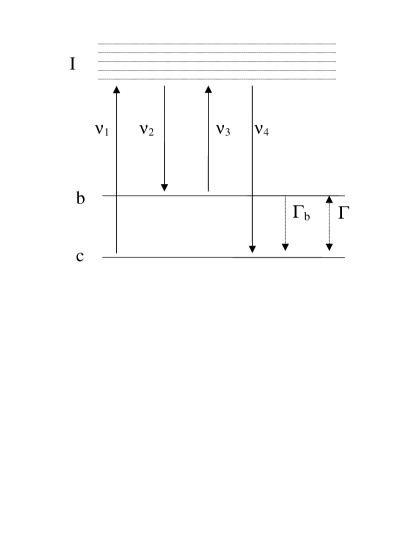
Figure 1: CARS scheme with three input fields of frequency $\nu_{1}$, $\nu_{2}$ and $\nu_{3}$ and a generated signal field $\nu_{4}=\nu_{1}+\nu_{3}-\nu_{2}$. The radiative damping rate from level $b$ to level $c$ is $\Gamma_{b}$ and the dephasing rate of the coherence between levels $b$ and $c$ is $\Gamma$.

II Nonlinear Interaction

We will consider stimulated Raman scattering involving three input fields ${\hat{a}}_{1},{\hat{a}}_{2},{\hat{a}}_{3}$ and one generated field ${\hat{a}}_{4}$ with corresponding frequencies $\nu_{i=1,2,3,4}$. The interaction Hamiltonian is written in terms of the two Raman-coupled atomic or molecular levels $|b\rangle$ and $|c\rangle$, of energies $\hbar\omega_{b}$ and $\hbar\omega_{c}$, and lowering operator $\hat{\sigma}=|c\rangle\langle b|$

$$\hat{V}=\hbar\left(R_{12}\hat{a}_{1}\hat{a}_{2}^{\dagger}+R_{43}\hat{a}_{3}^{\dagger}\hat{a}_{4}\right)\hat{\sigma}^{\dagger}e^{it\Delta}+H.a.$$ (1)

Here and elsewhere the time arguments will be suppressed where obvious in order to reduce clutter. The exponential factor signifies that all operators are in the interaction picture, its argument $\Delta=\omega_{bc}+\nu_{21}=\omega_{bc}+\nu_{34}$ with $\omega_{bc}=\omega_{b}-\omega_{c}$. These particular combination of atomic and field frequencies in $\Delta$ implies that the Hamiltonian contains only Raman resonant terms and excludes all non-resonant terms. For the case of FAST CARS where $\nu_{1}$ and $\nu_{2}$ pulses interact with the atoms before $\nu_{3}$, the non-resonant terms are simply not present. However when all the fields are present simultaneously the permutations of the fields lead to $24$ terms in the perturbation expansion which all contribute at the same order Laserna ; in that case we have in effect neglected the $20$ remaining terms which have non-resonant combinations of the fields and the atomic levels. If we are close to resonance this is certainly justified, in fact we will assume perfect two photon Raman resonance in this paper.

The Raman coupling constants are defined by $R_{12}=R_{12}^{{}^{\prime}}{\cal E}_{1}{\cal E}_{2}^{*}$

$$R_{12}^{{}^{\prime}}=\frac{-1}{\hbar^{2}}\sum_{j}\left[\frac{(\vec{\mu}_{fj}\cdot\vec{\varepsilon}_{1})(\vec{\mu}_{ji}\cdot\vec{\varepsilon}_{2})}{(\omega_{jc}+\nu_{2})}+\frac{({\vec{\mu}}_{fj}\cdot\vec{\varepsilon}_{2})(\vec{\mu}_{ji}\cdot\vec{\varepsilon}_{1})}{(\omega_{jc}-\nu_{1})}\right]$$ (2)

and likewise for $R_{43}$. The $\vec{\varepsilon}$ are unit polarization of the fields, $\vec{\mu}$ the dipole moments, $j$ labels the intermediate states and ${\cal E}_{l}=\sqrt{(\hbar\nu_{l})/(2\epsilon_{0}\epsilon_{p}V)}$ are the field quantization factors over volume $V$ in a medium of dielectric constant $\epsilon_{p}$ taken to be about the same for all laser fields. The decoherence rate between levels $b$ and $c$ is denoted by $\Gamma$ and the depopulation rate from level $b$ to level $c$ by $\Gamma_{b}$; damping to other levels is assumed negligible.

It will help to establish a relation with macroscopic quantities. The classical field amplitudes are $E_{i}={\cal E}_{i}\alpha_{i}$ for coherent state expectations $\alpha_{i}=\langle\hat{a}_{i}\rangle$. The third-order susceptibility is defined to be

$$\chi^{(3)}(-\nu_{4},\nu_{1},-\nu_{2},\nu_{3}) = -\hbar\frac{R_{43}^{{}^{\prime}*}R_{12}^{{}^{\prime}}}{(\Delta-i\Gamma)}\frac{N}{V},$$ (3)

with expected population difference between the two levels $N=N_{b}-N_{c}$. The Maxwell equation for the slowly varying amplitude of the generated field is

$$\left(\frac{\partial}{\partial t}+v\frac{\partial}{\partial z}\right)E_{4}=\frac{i\nu_{4}}{2\epsilon_{0}\epsilon_{p}}\chi^{(3)}E_{1}E_{2}^{*}E_{3},$$ (4)

with the velocity in the medium $v=c/\sqrt{\epsilon_{p}}$.

III Langevin Equations of motion

The three input fields $\nu_{1},\nu_{2}$ and $\nu_{3}$ are typically strong laser fields far above threshold, we will treat them as classical fields and replace $\hat{a}_{1(2,3)}\rightarrow\alpha_{1(2,3)}$. Considerable simplification is achieved by defining

$$\hat{A}(t) = \frac{R_{12}\alpha_{1}\alpha_{2}^{*}+R_{43}\alpha_{3}^{*}\hat{a}_{4}(t)}{g}$$

$$\xi = \frac{R_{12}\alpha_{1}\alpha_{2}^{*}}{g},\hskip 56.9055ptg=|R_{43}\alpha_{3}^{*}|.$$ (5)

The normalization $g$ has been chosen such that $\hat{A}(t)$ satisfies the boson commutation rules. Thus we can treat $\hat{A}(t)$ like a photon field operator. The parameters $g$ and $\xi$ being dependent only on the input fields will treated as constants in our calculations. The Heisenberg-Langevin equations of motion for the atomic operators are obtained from the interaction Hamiltionian:

$$\dot{\hat{\sigma}} = -(\Gamma+i\Delta)\hat{\sigma}+ig[\hat{\sigma}_{b}-\hat{\sigma}_{c}]\hat{A}+\hat{F}_{\sigma}$$

$$\dot{\hat{\sigma}}_{b} = -\Gamma_{b}\hat{\sigma}_{b}+ig\left[\hat{A}^{\dagger}\hat{\sigma}-\hat{\sigma}^{\dagger}\hat{A}\right]+\hat{F}_{b}$$

$$\dot{\hat{\sigma}}_{c} = \Gamma_{b}\hat{\sigma}_{b}-ig\left[\hat{A}^{\dagger}\hat{\sigma}-\hat{\sigma}^{\dagger}\hat{A}\right]+\hat{F}_{c}.$$ (6)

The coherence operator here differs from that in Eq. (1) by a phase factor $\hat{\sigma}(t)e^{-i\Delta t}\rightarrow\hat{\sigma}(t)$, and $\hat{\sigma}_{b(c)}$ are the population operators for the atomic levels. The $\hat{F}$’s are the Langevin noise operators. They have vanishing first moments $\langle\hat{F}(t)\rangle=0$, since the entropy of the system cannot be lowered by noise Reichl . The second moments are taken to be delta-correlated in time corresponding to Markovian white noise

$$\langle\hat{F}_{i}(t)\hat{F}_{j}(t^{\prime})\rangle=2D_{ij}\ \delta(t-t^{\prime}).$$ (7)

The $D_{ij}$ are the diffusion coefficients in analogy with classical Langevin equations. The diffusion coefficients associated with Eqs. (III) are calculated using the generalized fluctuation-dissipation theorem Louisell in Appendix A.

The Langevin equation for the signal field operator is

$$\dot{\hat{a}}_{4} = -\gamma\hat{a}_{4}-iR_{43}^{*}\alpha_{3}\hat{\sigma}+\hat{F}_{a_{4}}.$$ (8)

Here we included an heuristic field damping rate $\gamma$ to allow for atom-field interaction inside a cavity. From this equation, we can construct the equation

$$\dot{\hat{A}}=-\gamma(\hat{A}-\xi)-ig\hat{\sigma}.$$ (9)

The effects of a thermal heat bath that accounts for a non-vanishing $\hat{F}_{a_{4}}$ are neglected by assuming low temperature. In this paper we will also assume two photon Raman resonance thereby set $\Delta=0$.

We next define macroscopic variables by summing over the operators for all the particles (atoms/molecules) in the medium

$$\hat{M}=-i\sum\hat{\sigma}\hskip 28.45274pt\hat{N}_{b(c)}=\sum\hat{\sigma}_{b(c)}$$ (10)

and the population sum and difference operators $\hat{N}_{T}=\hat{N}_{b}+\hat{N}_{c}$ and $\hat{N}=\hat{N}_{b}-\hat{N}_{c}$. The equations of motion for the collective atomic variables and the field are then

$$\dot{\hat{M}} = -\Gamma\hat{M}+g\hat{N}A+\hat{F}_{M}$$

$$\dot{\hat{N}} = -\Gamma_{b}(\hat{N}+\hat{N}_{T})-2g[\hat{A}^{*}\hat{M}+\hat{M}^{*}\hat{A}]+{\hat{F}}_{N}$$

$$\dot{\hat{N}}_{T} = 0$$

$$\dot{\hat{A}} = -\gamma(\hat{A}-\xi)+g\hat{M},$$ (11)

with the total number of active particles $\langle\hat{N}_{T}\rangle$ being conserved. The associated diffusion coefficients are shown in Appendix A.

Solution of these equations is facilitated by transforming them into equivalent c-number equations Kolobov ; Fleischhauer ; SZ . This is achieved by putting all the operators in normal order chosen to be $\hat{A}^{\dagger},\hat{M}^{\dagger},\hat{N},\hat{M},\hat{A}$ which establishes an unique correspondence between the quantum and classical equations. Since the equations are already in normal order the operators are simply replaced with their classical counterparts ${\cal A}^{*},{\cal M}^{*},{\cal N},{\cal M},{\cal A}$.

The c-number noise functions satisfy $\langle{\cal F}(t)\rangle=0$ and $\langle{\cal F}(t){\cal F}(t^{\prime})\rangle=2{\cal D}\delta(t-t^{\prime})$ just like their operator counterparts. The c-number diffusion coefficients will however acquire additional terms arising from normal ordering; all the non-vanishing coefficients are listed in Appendix A. The corresponding properties of the noise in the frequency domain are summarized in Appendix B. It is worth mentioning here that the expectations in the c-number representation are now in the Glauber-Sudarshan P-representation of a thermal distribution which happens to be a Gaussian distribution of zero mean. This means that the Gaussian moment theorem applies and the first and second moments suffice to determine the distribution completely.

IV Equations and assumptions of the model

We consider small fluctuations about the mean values for both atomic and field variables ${\cal M}(t)={\cal M}_{0}(t)+\delta{\cal M}(t)$, ${\cal N}(t)={\cal N}_{0}(t)+\delta{\cal N}(t)$ and ${\cal A}(t)={\cal A}_{0}(t)+\delta{\cal A}(t)$. It is convenient to define two real variables ${\cal T}(t)={\cal M}^{*}(t){\cal A}_{0}(t)+{\cal M}(t){\cal A}_{0}^{*}(t)$ and ${\cal S}(t)=|{\cal A}(t)|^{2}$, with linearized fluctuations

$$\delta{\cal S}(t) = {\cal A}_{0}(t)\delta A^{*}(t)+{\cal A}_{0}^{*}(t)\delta A(t)$$

$$\delta{\cal T}(t) = {\cal A}_{0}(t)\delta M^{*}(t)+{\cal A}_{0}^{*}(t)\delta M(t)$$

$${\cal F_{T}}(t) = {\cal A}_{0}(t){\cal F_{M}}^{*}(t)+{\cal A}_{0}^{*}(t){\cal F}_{{\cal M}}(t).$$ (12)

The relation to the properties of the generated field $\alpha_{4}$ that we are finally interested in are as follows: The strength of the signal field, given by the number of generated photons, and the atomic noise in the photon number, quantified by its variance, are determined by

$$n_{4}(t) = \langle\alpha_{4}^{*}(t)\alpha(t)\rangle=|{\cal A}_{0}(t)-\xi|^{2}$$

$$\delta n_{4}^{2}(t) = \frac{n_{4}(t)}{|{\cal A}_{0}(t)|^{2}}\langle\delta{\cal S}^{2}(t)\rangle.$$ (13)

To reduce clutter we will often leave out the expectation brackets being obvious from the context. The variance is obviously linearized and neglects relatively small terms quadratic in the correlations. We will primarily consider regimes where the generated field $\alpha_{4}$ is much weaker than the input fields (as we justify numerically in Sec. VII.2) and therefore we will replace $|{\cal A}_{0}|^{2}\simeq|\xi|^{2}$ where appropriate and consistent.

IV.1 adiabatic elimination of the averages of atomic variables

Since the fluctuations have vanishing average, we can write separate equations for the mean and the linear fluctuations. The equations for the averages can be had by simply leaving out the Langevin forces

$$\partial_{t}{\cal M}_{0} = -\Gamma{\cal M}_{0}+g{\cal N}_{0}{\cal A}_{0}$$

$$\partial_{t}{\cal N}_{0} = -\Gamma_{b}({\cal N}_{0}+N_{T})-2g[{\cal A}_{0}^{*}{\cal M}_{0}+{\cal M}_{0}^{*}{\cal A}_{0}]$$

$$\partial_{t}{\cal A}_{0} = -\gamma({\cal A}_{0}-\xi)+g{\cal M}_{0}.$$ (14)

Atomic/molecular transitions typically occur on a faster time scale than the variations in a radiation field, which means that the medium will adiabatically follow the field for weak coupling. Even when using fast pulses, the coherence generating pulses can be taken to be of sufficiently long duration for this to be true. Therefore taking averages over intermediate time scales, the time-derivatives in the equations for the averages of the medium variables ${\cal M}_{0}$ and ${\cal N}_{0}$ may be neglected in what is called adiabatic elimination Louisell and we obtain algebraic relations for the coarse-grained averages:

$${\cal N}_{0}=-\frac{N_{T}}{1+B|\xi|^{2}},\ \ {\cal M}_{0}=-\frac{C}{g}\frac{{\cal A}_{0}}{1+B|\xi|^{2}}$$ (15)

where we set $|{\cal A}_{0}|^{2}\simeq|\xi|^{2}$ as discussed earlier. We define some parameters here that we will use often and which will serve to simplify our expressions considerably:

$$B=\frac{4g^{2}}{\Gamma_{b}\Gamma},\hskip 28.45274ptC=\frac{N_{T}g^{2}}{\Gamma}.$$ (16)

The parameter $B$ is dimensionless and $C$ carries the dimension of inverse time. As we corroborate numerically later $B|\xi|^{2}\ll 1$, so the upper level is never strongly populated, ${\cal N}_{0}\simeq-N_{T}$ and we can simplify by setting $1+B|\xi|^{2}\simeq 1$ in the rest of the paper. Substituting the atomic mean values we get an uncoupled equation for the average of the field variable

$$\partial_{t}{\cal A}_{0}=-\gamma({\cal A}_{0}-\xi)-C{\cal A}_{0}.$$ (17)

IV.2 fluctuations

In describing the fluctuations, we cannot make arguments for adiabatic elimination of the medium variables as we did for the averages; this is due to the presence of the rapidly varying noise functions. An attempt to make such an approximation can lead to unphysical divergences in the correlations; we will discuss this issue in some detail in Appendix D. Therefore we solve coupled equations for the fluctuations for both the field and the medium. We write the relevant equations in terms of the variables ${\cal T}$ and ${\cal S}$

$$\partial_{t}\delta{\cal T} = -\Gamma\delta{\cal T}+2g\delta{\cal N}|{\cal A}_{0}|^{2}+g{\cal N}_{0}\delta{\cal S}+{\cal F_{T}}$$

$$\partial_{t}\delta{\cal N} = -\Gamma_{b}\delta{\cal N}+2C\delta{\cal S}-2g\delta{\cal T}+{\cal F}_{\cal N}$$

$$\partial_{t}\delta{\cal S} = -\gamma\delta{\cal S}+g\delta{\cal T}.$$ (18)

In writing these equations, we have treated ${\cal A}_{0}$ as a constant. We will see that in all the cases we consider in this paper this assumption is valid, because either ${\cal A}_{0}$ will have an unvarying steady state value or it will satisfy ${\cal A}_{0}\simeq\xi$, even as a function of position when propagation in free space is inovlved (see next subsection). It is clear from the equations above that the fluctuations can be fully expressed in terms of the correlations of the variables ${\cal T}$ and $\cal N$. Using the results in Appendix A, we find that the two variables are uncorrelated with each other but the strengths of their autocorrelations are specified by the diffusion coefficients

$$2{\cal D}_{{\cal T}{\cal T}} = 2(\Gamma-\Gamma_{b})N_{T}B|\xi|^{4}$$

$$2{\cal D}_{{\cal N}{\cal N}} = 4\Gamma_{b}N_{T}B|\xi|^{2}$$ (19)

where we used the expressions for the averages in Eq. (15). In writing these expressions we used the weak field approximation ${\cal A}_{0}\simeq\xi$ and the assumption of weak upper level occupation $B|\xi|^{2}\ll 1$, and therefore in effect we can treat these coefficients as constants.

IV.3 Free space description

The equations above are appropriate for describing experiments conducted in a cavity of damping rate $\gamma$. However if we wish to describe experiments in free space we have to allow for field propagation through the medium and effectively replace $\gamma\rightarrow v\partial_{z}$ . An approach discussed by Drummond and Carter Drummond ; Fleischhauer outlined in Appendix C, leads to the appropriate space-time equation for the field variable

$$(\partial_{t}+v\partial_{z}){\cal A}(z,t)=g{\cal M}(z,t).$$ (20)

This equation follows from Eq. (91) derived in the appendix, on assuming that all the input fields propagate collinearly in the z-direction and their amplitudes $\alpha_{1(2,3)}$ vary little over the interaction length $L$, i.e. the length of the region over which the fields interact with the atoms, and therefore may be treated as constants.

Thus for experiments in free space, equations for the field variable in (17) and (18) are modified to

$$(\partial_{t}+v\partial_{z}){\cal A}_{0}(z,t) = -C{\cal A}_{0}(z,t)$$

$$(\partial_{t}+v\partial_{z})\delta{\cal S}(z,t) = g\delta{\cal T}(z,t).$$ (21)

The equations for the atomic variables are formally unchanged, but they now carry both position and time argument $(z,t)$; their spatial dependence arises through their interdependence on the field variable.

V Pulsed Inputs

We first consider the case where the input laser fields are extremely short and fast pulses. In particular we take the pulses to arrive in sequence as is the case in FAST CARS fastcars ; the fields $\alpha_{1}$ and $\alpha_{2}$ are allowed to interact first with the atoms for a duration $\Delta t_{c}$ creating the coherence, then after a delay $\Delta t_{d}$ the field $\alpha_{3}$ occurs for time $\Delta t_{3}$. This means that the atomic variables can now only depend on the first two fields, so we replace ${\cal A}_{0}\rightarrow\xi$ in Eqs. (17) and (IV.2) and also set $\delta{\cal S}=0$ in the equations for the fluctuations of atomic variables:

$$\partial_{t}\delta{\cal T} = -\Gamma\delta{\cal T}+2g\delta{\cal N}|\xi|^{2}+{\cal F_{T}}$$

$$\partial_{t}\delta{\cal N} = -\Gamma_{b}\delta{\cal N}-2g\delta{\cal T}+{\cal F}_{\cal N}.$$ (22)

The main premise for this scenario is that when a rapid sequence of fast femtosecond pulses are used, the field $\alpha_{3}$ scatters off the generated coherence before it has time to decay significantly. Thus for time intervals such that $\Delta t_{d}+\Delta t_{3}\ll\Gamma^{-1},\Gamma_{b}^{-1}$ the generated coherence may be taken to be constant. For longer durations however we have to allow for decay of the coherence ${\cal M}_{0}$ in Eq. (15).

During the signal-generating cycle when $\alpha_{3}$ is present the mean coherence is described by

$$\partial_{t}{\cal M}_{0} = -\Gamma{\cal M}_{0}-g({\cal A}_{0}-\xi){\cal N}_{0}.$$ (23)

After the coherence generating pulses are turned off, the value of generated coherence from Eq. (15) ${\cal M}_{0}(0)=g\xi{\cal N}_{0}/\Gamma$ can be taken as the initial value of the coherence in the above equation (if $\Delta t_{d}\simeq 0$) and since initially there is no signal field ${\cal A}_{0}(0)=\xi$. It is then easy to see that the ratio of the magnitude of the first term to that of the second term is $\sim|\xi|/|{\cal A}_{0}-\xi|$ which is large for weak generated field and short duration pulses. Therefore we can neglect the second term and take the driving coherence to simply decay exponentially from the moment the generating fields are turned off ${\cal M}_{0}(t)={\cal M}_{0}(0)e^{-\Gamma t}$.

The equation for the average field then becomes

$$\partial_{t}{\cal A}_{0}=-\gamma({\cal A}_{0}-\xi)-C\xi e^{-\Gamma t}.$$ (24)

The fluctuations will likewise decay since the diffusion coefficients depend on the averages ${\cal N}_{0}$ and ${\cal M}_{0}$. The diffusion coefficients in Eq. (IV.2) will then have an exponentially decaying time dependence, ${\cal D_{NN}}\sim e^{-\Gamma_{b}t}$ and ${\cal D_{TT}}\sim e^{-\Gamma t}$. We note however that there is no constraint on the duration $\Delta t_{c}$ of the coherence generating pulses, so they can be taken to be sufficiently long to create a steady state value of the coherence before they are turned off, thereby justifying adiabatic elimination.

V.1 pules: interaction in a cavity

The mean value of the field variable after the third pulse ${\cal A}_{0}(\Delta t_{3})$ is easily obtained by integrating Eq. (24)

$${\cal A}_{0}(\Delta t_{3})-\xi=-C\xi\times\frac{e^{-\Gamma\Delta t_{3}}-e^{-\gamma\Delta t_{3}}}{\gamma-\Gamma}.$$ (25)

The phase of ${\cal A}_{0}$ is given by that of $\xi$, since ${\cal A}_{0}/\xi$ is real. When the duration of the third pulse is short $\Delta t_{3}\ll\Gamma^{-1}$,

$${\cal A}_{0}(\Delta t_{3})-\xi\simeq-C\xi\Delta t_{3}.$$ (26)

The equal time fluctuations of the field are given by

$$\delta{\cal S}^{2}(\Delta t_{3})=g^{2}\int_{0}^{\Delta t_{3}}dt\int_{0}^{\Delta t_{3}}dt^{\prime}e^{-\gamma(2\Delta t_{3}-t-t^{\prime})}\langle\delta{\cal T}(t)\delta{\cal T}(t^{\prime})\rangle$$ (27)

In order to evaluate this we first take a Fourier transform of the Eqs. (22), the relevant definitions and properties of the fluctuations and noise in the frequency domain are described in Appendix B:

$$(\Gamma-i\omega)\delta{\cal T}(\omega) = 2g|\xi|^{2}\delta{\cal N}(\omega)+{\cal F_{T}}(\omega)$$

$$(\Gamma_{b}-i\omega)\delta{\cal N}(\omega) = -2g\delta{\cal T}(\omega)+{\cal F}_{\cal N}(\omega)$$ (28)

which we then solve to get

$$\delta{\cal T}(\omega)\simeq\frac{\left[2g|\xi|^{2}{\cal F}_{{\cal N}}+(\Gamma_{b}-i\omega){\cal F_{T}}\right]}{(\Gamma-i\omega)(\Gamma_{b}-i\omega)}.$$ (29)

Assuming weak excitation we set $|1+\frac{4g^{2}\xi^{2}}{[\Gamma-i\omega][\Gamma_{b}-i\omega]}|^{2}\simeq 1$. Using this expression for $\delta{\cal T}(\omega)$ we can evaluate the integrals in Eq. (27). The details of the calculations are shown in Appendix E. The general result result derived there is not particularly illuminating, instead here we consider the relevant limiting cases. In the short pulse limit $\Delta t_{3}\ll\Gamma^{-1}$, we found that a Taylor expansion leads to an exact cancellation of the terms linear in $\Delta t_{3}$ and we get a quadratic dependence on the interaction time

$$\delta{\cal S}^{2}(\Delta t_{3})\simeq\frac{g^{2}\Delta t_{3}^{2}}{2}\left[\frac{B|\xi|^{4}2{\cal D_{NN}}}{(\Gamma+\Gamma_{b})}+\frac{2{\cal D_{TT}}}{\Gamma}\right].$$ (30)

A conspicuous feature of this limit is that $\gamma$ is absent in the expressions for both the mean and the fluctuation. Thus for pulses of duration shorter than the cavity damping time, the presence of the cavity has no effect on the signal or its associated noise due to the medium. This short pulse limit implies the hierarchy of time scales $\gamma^{-1}\gg\Gamma^{-1},\Gamma_{b}^{-1}\gg\Delta t_{3}$.

In the opposite limit of long pulse duration $\Delta t_{3}\gg\gamma^{-1}\gg\Gamma^{-1},\Gamma_{b}^{-1}$ the fluctuation is approximately

$$\delta{\cal S}^{2}(\Delta t_{3})\simeq\frac{g^{2}\Delta t_{3}^{2}e^{-\Gamma\Delta t_{3}}}{2}\left[\frac{2{\cal D_{NN}}}{\Gamma\Gamma_{b}\gamma}B|\xi|^{4}+\frac{2{\cal D_{TT}}}{\Gamma^{2}\gamma}\right].$$ (31)

Here we set the depopulation rate and decoherence rates to be equal $\Gamma\simeq\Gamma_{b}$, to mask unnecessary details and highlight the main feature, which is that both the mean and the fluctuations essentially vanish towards the end of a long third pulse as the driving coherence disappears. The conclusion is that, regardless of the duration of the third pulse, significant signal field is generated only during times satisfying $<\Gamma^{-1},\Gamma_{b}^{-1}$.

V.2 pulses: interaction in free space

The last subsection showed that increasing the duration of the interaction between the third pulse and the atoms will make a difference only upto a point, since we are limited by the decay time of the coherence. In free space, this means that we will not get a stronger sustained signal by simply increasing the interaction length L. Therefore we will confine ourselves to sample sizes $L<v\Gamma^{-1},v\Gamma_{b}^{-1}$, and we will use Eq. (21) where, taking the coherence to remain unchanged during the time of interaction, we set ${\cal A}_{0}(z,t)\rightarrow\xi$.

A time-frequency Fourier transform and subsequent integration over the interaction length gives

$$(-i\omega+v\partial_{z}){\cal A}_{0}(z,\omega) = -C\xi\delta(\omega)$$ (32)

$$\Rightarrow{\cal A}_{0}(L,\omega) = e^{i\omega L/v}\xi\left[1-C\frac{L}{v}\right]$$

and an inverse transform yields the delta-function $\delta(t-L/v)$ that simply tells us that time is a redundant parameter and the field can be specified by its position alone

$${\cal A}_{0}(L) = \xi-C\xi\frac{L}{v}.$$ (33)

Likewise for the variance we consider the equations for the fluctuations in the frequency domain. Since we set ${\cal A}_{0}(z,t)\simeq\xi$, the equations are given simply by (28). Substituting the expression $\delta{\cal T}(\omega)$ from Eq. (29) into the equation for the field fluctuation

$$-i\omega+v\partial_{z}\delta{\cal S}(z,\omega)=g\delta{\cal T}(z,\omega),$$ (34)

and integrating over the interaction length $L$ we get the spectral density of the noise

$$\delta S^{2}(L,\omega)=\frac{1}{2\pi}\frac{L^{2}}{v^{2}}\frac{\left[4g^{4}|\xi|^{4}2{\cal D_{NN}}+g^{2}(\Gamma_{b}^{2}+\omega^{2})2{\cal D_{TT}}\right]}{(\Gamma^{2}+\omega^{2})(\Gamma_{b}^{2}+\omega^{2})}.$$

The autocorrelation at equal times obtained by doing a partial fraction decomposition and an inverse Fourier transform defines the variance

$$\delta S(L)^{2}=\frac{g^{2}L^{2}}{2v^{2}}\left[\frac{B|\xi|^{4}2{\cal D_{NN}}}{(\Gamma+\Gamma_{b})}+\frac{2{\cal D_{TT}}}{\Gamma}\right].$$ (35)

We see that both the mean and the variance are identical to what we found in the short pulse limit when the interaction took place inside a cavity, bearing in mind that here $L/v$ defines the time of interaction. This reaffirms the conclusion that for short pulses there is no real advantage in using a cavity.

VI Continuous Wave (cw) Inputs

We now consider the cases where all three input fields occur continuously and simultaneously. In this case steady state values for the medium variables may be considered, and their decay does not put limits on the interaction time as it did previously when using sequential pulses. But the calculation of fluctuations is complicated by the fact that the equations for the medium variables and the field variable do not decouple as they did for sequential pulses.

VI.1 cw: interaction in a cavity

The average is found by integrating Eq. (17), exactly in the form it is written, with the initial condition ${\cal A}_{0}(0)=\xi$,

$${\cal A}_{0}(t)-\xi=-C\xi\times\frac{1-e^{-(\gamma+C)t}}{(\gamma+C)}.$$ (36)

Unlike the pulsed case there are no obvious time constraints, except those arising from possible damage to the sample by prolonged exposure to the fields, so we can take the long time limit $t\rightarrow\infty$ and we get a steady state signal

$${\cal A}_{0}-\xi=-C\xi\times\frac{1}{(\gamma+C)}.$$ (37)

We note that if $\gamma\ll C$ the generated field essentially vanishes, which suggests that we need to have $\gamma\geq C$. In that case we can further use the assumption of weak signal field to conclude that

$$\frac{{\cal A}_{0}-\xi}{\xi}\simeq\frac{C}{\gamma}\ll 1\hskip 14.22636pt\Rightarrow{\cal A}_{0}-\xi\simeq-C\xi\frac{1}{\gamma}.$$ (38)

The fluctuations are best determined by writing the three coupled equations in the frequency domain in matrix form:

$$\left[\begin{array}[]{ccc}(\Gamma-i\omega)&-2g|{\cal A}_{0}|^{2}&-g{\cal N}_{0}\\ 2g&(\Gamma_{b}-i\omega)&-2C\\ -g&0&(\gamma-i\omega)\end{array}\right]\left[\begin{array}[]{c}\delta{\cal T}\\ \delta{\cal N}\\ \delta{\cal S}\end{array}\right]=\left[\begin{array}[]{c}{\cal F}_{{\cal T}}\\ {\cal F}_{{\cal N}}\\ 0\end{array}\right].$$ (48)

Inverting the coefficient matrix ${\bf M_{F}}$ gives the solution

$$\delta{\cal S}(\omega) = \frac{\left[(\Gamma_{b}-i\omega)g{\cal F_{T}}(\omega)+2g^{2}|{\cal A}_{0}|^{2}{\cal F_{N}}(\omega)\right]}{\det{\bf M_{F}}}$$ (49)

$$\det{\bf M_{F}} \simeq (\Gamma-i\omega)(\Gamma_{b}-i\omega)(\gamma-i\omega).$$

In computing the determinant in the denominator we introduced some simplifications using the arguments leading upto Eq. (38) and we neglected the frequency dependence in the term proportional to $B|{\cal A}_{0}|^{2}$ [refer to the comment following Eq. (29)] . Squaring this gives the power spectrum (Appendix B) and then a Fourier transform and the adiabatic assumption $\gamma\ll\Gamma,\Gamma_{b}$ yields the steady state fluctuations

$$\delta{\cal S}^{2}(t)\simeq\frac{g^{2}}{2\gamma}\left[\frac{2{\cal D_{NN}}}{\Gamma\Gamma_{b}}B|\xi|^{4}+\frac{2{\cal D_{TT}}}{\Gamma^{2}}\right].$$ (50)

While the adiabatic assumption was not necessary it gave a simpler expression, the more general expression is shown in Appendix E. What sets this case apart from the rest is that both the signal field and the variance in the steady state depend on the cavity lifetime, $\gamma^{-1}$ and that dependence is linear.

VI.2 cw: interaction in free space

In order to find the signal strength, we do a Fourier transform of Eq (21)

$$(-i\omega+v\partial_{z}){\cal A}_{0}(z,\omega) = -C{\cal A}_{0}(z,\omega)$$ (51)

and integrate it over the interaction length $L$ to get

$${\cal A}_{0}(L,\omega) = e^{i\omega L/v}{\cal A}_{0}(0,\omega)e^{-CL/v}.$$ (52)

As in the analogous case in a cavity, the time parameter is seen to be redundant after an inverse Fourier transform and we get simply

$${\cal A}_{0}(L) = \xi e^{-CL/v}.$$ (53)

In calculating the fluctuations we take the Fourier transform of the equations for the atomic variables as they appear in Eqs. (18) and the field fluctuation as it appears in (21), keeping in mind that all the fluctuation and noise elements will thereafter carry an argument of $(z,\omega)$. The three coupled equations yield an equation for the field fluctuation

$$[v\partial_{z}-i\omega-{\cal G}(\omega)]\delta{\cal S}\simeq\frac{g\left[2g|\xi|^{2}{\cal F}_{{\cal N}}+(\Gamma_{b}-i\omega){\cal F_{T}}\right]}{(\Gamma-i\omega)(\Gamma_{b}-i\omega)}$$

$${\rm with}\ \ {\cal G}(\omega)\simeq\frac{g\left[4gC|\xi|^{2}+(\Gamma_{b}-i\omega)g{\cal N}_{0}\right]}{(\Gamma-i\omega)(\Gamma_{b}-i\omega)}.\hskip 14.22636pt$$ (54)

We integrate this with respect to the spatial coordinate $z$, and thereby we get the spectral density

$$\delta S^{2}(L,\omega) = \frac{1}{2\pi}\frac{L}{v}\times\frac{1-e^{2Re[{\cal G}(\omega)]\frac{L}{v}}}{-2Re[{\cal G}(\omega)]}$$

$$\times\frac{4g^{4}|\xi|^{4}2{\cal D_{NN}}+g^{2}(\Gamma_{b}^{2}+\omega^{2})2{\cal D_{TT}}}{(\Gamma^{2}+\omega^{2})(\Gamma_{b}^{2}+\omega^{2})}.$$

We use $B|\xi|^{2}\ll 1$ to simplify

$$2Re[{\cal G}(\omega)] \simeq -\frac{2C\Gamma^{2}}{(\Gamma^{2}+\omega^{2})}.$$ (55)

We note this quantity achieves the largest magnitude when $\omega=0$. In the case of short interaction length $CL/v\ll 1$ both the signal and the variance resemble those we got in the case of pulsed inputs in free space

$${\cal A}_{0}(L) \simeq \xi-C\xi\frac{L}{v}$$ (56)

$$\delta S^{2}(L,\omega) \simeq \frac{1}{2\pi}\frac{L^{2}}{v^{2}}\frac{\left[4g^{4}|\xi|^{4}2{\cal D_{NN}}+g^{2}(\Gamma_{b}^{2}+\omega^{2})2{\cal D_{TT}}\right]}{(\Gamma^{2}+\omega^{2})(\Gamma_{b}^{2}+\omega^{2})}.$$

In the opposite time limit of long interaction length $CL/v\gg 1$, we find that the expression for the average value of the field variable ${\cal A}_{0}$ tends to become increasingly smaller. Equation (53) tells us

$$n_{4}(L)=|{\cal A}_{0}(L)-\xi|^{2} = |\xi(1-e^{-CL/v})|^{2},$$ (57)

so that in this limit the input fields vanish and give way to the signal field. Our model however does not allow us to obtain an accurate expression for the variance in this limit. This is because the equations (18) were based on the assumption that ${\cal A}_{0}$ does not change significantly and the generated field is relatively weak, and this is no longer true when $L$ becomes large. Yet based on the fact that average value ${\cal A}_{0}$ decreases over the length $L$ and hence the diffusion coefficients also decrease, we could expect that the noise contribution from the active medium will actually be lower farther along the interaction length.

VII Discussion of Results, Inferences and Assumptions

We will now discuss in some detail the physical implications of the results we obtained in the previous sections, and also elaborate a bit more on our assumptions and some associated subtleties that we touched on while deriving those results. We begin by considering realistic numerical values for our parameters and variables and thereby provide concrete justification for the approximations we made.

VII.1 Numerical Estimates

For the purpose of numerical estimation we will use the specific example of an anthrax spore for which the Raman active molecule is dipicolinic acid (DPA) which constitutes $17\%$ of the weight, the rest being mainly water. The number density of DPA molecules in an anthrax spore is $N_{T}\sim 4\times 10^{26}$ molecules m^-3, and the dimensions of the spore itself is $1\times 2\times 1\ {\rm\mu m}^{3}$. We will take all optical frequencies to be in the visible range $\nu\sim 2\pi c/\lambda\simeq 4\times 10^{15}$.

Since some of the properties of DPA are not easily available, for those properties we will use the values for benzene, an organic molecule that has a similar structure. Thus for instance we use the spontaneous Raman differential cross-section for Benzene $\frac{d\sigma}{d\Omega}=32.5\times 10^{-34}{\rm m^{2}/sr/molecule}$, and we take the linewidths of Raman transitions in Benzene to estimate $\Gamma_{b}\sim 10^{11}{\rm Hz}$.

We first determine the strength of the Raman coupling $R^{\prime}_{ij}$, we can do that in two ways, assuming in either case that only a few intermediate states contribute: first using Eq. (2), and taking $\mu\sim ea_{0}$ with $a_{0}$ being the Bohr radius

$$|R^{\prime}_{ij}|\sim\frac{\mu^{2}}{\hbar^{2}\nu}\simeq 4\times 10^{-6}{\rm C}^{2}{\rm m}^{2}/{\rm J}^{2}{\rm s};$$ (58)

and secondly using the Kramers-Heisenberg formula for the differential scattering cross-section applied to spontaneous Raman scattering

$$|R^{\prime}_{ij}|\sim\frac{4\pi\epsilon_{0}c^{2}}{\hbar\nu^{2}}\sqrt{\frac{d\sigma}{d\Omega}}\simeq 0.35\times 10^{-6}{\rm C}^{2}{\rm m}^{2}/{\rm J}^{2}{\rm s}.$$ (59)

So we will take $|R^{\prime}_{ij}|\sim 10^{-6}\ {\rm C}^{2}{\rm m}^{2}/{\rm J}^{2}{\rm s}.$ Next we determine the field density and photon density from the expression for the field intensity (power/area)

$$I=\frac{1}{2}v\epsilon_{p}\epsilon_{0}|{\cal E}\alpha|^{2}=\frac{1}{4}v(\hbar\nu)\frac{|\alpha|^{2}}{V}.$$ (60)

For strong lasers we could take the typical intensities to be $I\sim 10^{12}$ Wm^-2, in which case we get

$$|{\cal E}\alpha|^{2}\sim 5\times 10^{14}{\rm N}^{2}{\rm C}^{-2},\hskip 8.53581pt\frac{n}{V}=\frac{|\alpha|^{2}}{V}\simeq 5\times 10^{22}{\rm m}^{-3}.$$ (61)

Taking all the input fields to have similar intensities and assuming natural linewidth $\Gamma_{b}\sim 10^{11}$ Hz and decoherence rate $\Gamma\sim 10^{13}-10^{14}$ Hz,

$$B|\xi|^{2}=\frac{4g^{2}}{\Gamma\Gamma_{b}}\sim\frac{4|R^{\prime}_{12}|^{2}|{\cal E}\alpha|^{2}}{\Gamma\Gamma_{b}}\sim 10^{-8}.$$ (62)

Indeed for this choice of parameters we are justified in taking the weak-excitation limit $B|\xi|^{2}\ll 1$, and in fact this will be valid till the field intensities increase to about $10^{16}$ Wm^-2; we note that this is the intensity level at which cascade breakdown of air occurs at STP Kroll , so our weak-field assumption covers most realistic regimes. Thus we are quite justified in setting $1+B|\xi|^{2}\simeq 1$.

Finally we address the issue of the interaction times, since many of our results assume short interaction times. In the case of pulsed inputs, $\Gamma^{-1}$ sets the limits on the pulse duration to be $\Delta t_{3}<10^{-13}$ s, which is certainly within the bounds of experimental capabilities using femtosecond pulses. In the case of propagation in free space, taking the dimension of an anthrax spore $L\sim 10^{-6}$ m as the interaction length we find $L/v\sim 10^{-15}<\Gamma^{-1}$. In either case the constraints of short interaction times are likely to be satisfied for physical regimes of interest.

VII.2 Signal and noise

The main observation we have from our calculations is that when the duration of interaction between the signal-generating field and the Raman-active medium $\Delta t=\Delta t_{3},L/v$ is short compared to $\Gamma^{-1}$, the signal and the noise due to the medium have essentially the same theoretical description independent of the various experimental scenarios that we considered:

$$n_{4} \simeq \xi^{2}C^{2}\Delta t^{2}\simeq\frac{N_{T}^{2}|R_{43}R_{12}|^{2}n_{1}n_{2}n_{3}\Delta t^{2}}{\Gamma^{2}}$$

$$\delta n_{4}^{2} \simeq \frac{g^{2}\Delta t^{2}}{2}\left[\frac{B|\xi|^{4}2{\cal D_{NN}}}{(\Gamma+\Gamma_{b})}+\frac{2{\cal D_{TT}}}{\Gamma}\right]$$ (63)

$$\simeq n_{4}^{2}\times\frac{8(\Gamma-\Gamma_{b})}{N_{T}\Gamma_{b}},$$

where we have used $B|\xi|^{2}\ll 1$ to set ${\cal N}_{0}\simeq N_{T}$ and $C\simeq C$; we also noted that the term involving ${\cal D_{NN}}$ is smaller by a factor of $B|\xi|^{2}$ than the one involving ${\cal D_{TT}}$ and hence we only retained the latter.

The exception to the above expressions was the case of continuous wave input in a cavity for which we got a steady state signal and noise given by:

$$n_{4} \simeq \frac{N_{T}^{2}|R_{43}R_{12}|^{2}n_{1}n_{2}n_{3}}{\Gamma^{2}}\frac{1}{\gamma^{2}}$$

$$\delta n_{4}^{2} \simeq n_{4}^{2}\times\frac{8\gamma(\Gamma-\Gamma_{b})}{N_{T}\Gamma\Gamma_{b}}.$$ (64)

The signal has the same form as the other cases with $\Delta t\rightarrow\gamma^{-1}$. But the fluctuations differ by a factor of $\gamma/\Gamma$. Since typically $\gamma\ll\Gamma$ the noise noise will be less in this case, and because $\gamma^{-1}$ is greater than the short time limits in the other cases the signal is bigger. In addition to this, the fact that there are no major constraints on the duration of the irradiations apart from their possible destruction of the sample, this scenario seems to be the best one from the signal to noise perspective. However that conclusion has to be moderated by the fact that when all three input fields happen simultaneously, there can be significant contributions from the non-resonant terms in our interaction Hamiltonian in Eq. (1), particularly if we cannot achieve two-photon Raman resonance. This is where the sequential pulse scheme as in FAST CARS has an advantage.

We can recast our expressions for the signal and fluctuations in terms of macroscopic variables. First using Eq. (3) and the definition of classical field amplitude $E_{l}={\cal E}_{l}\alpha_{l}$ we write the signal in terms of the classical field amplitudes:

$$|E_{4}|^{2} = \left(\frac{\nu_{4}}{2\epsilon_{0}\epsilon_{p}}\right)^{2}[\chi^{(3)}]^{2}|E_{1}|^{2}|E_{2}|^{2}|E_{3}|^{2}\times\Delta t^{2}$$ (65)

where $\Delta t=\Delta t_{3},L/v,\gamma^{-1}$ depending on the experimental configuration. Written this way we see that our expression for the signal is consistent with what we would get if we integrated the classical equation (4) for the slowly-varying amplitude with appropriate assumptions. A more practical representation would be in terms of the input intensities using Eq. (60)

$$I_{4} = \left(\frac{\nu_{4}}{c\epsilon_{0}^{2}}\right)^{2}[\chi^{(3)}]^{2}I_{1}I_{2}I_{3}\Delta t^{2}$$

$$\delta I_{4}^{2} = I_{4}^{2}\times\frac{8(\Gamma-\Gamma_{b})}{\Gamma_{b}N_{T}}\times\left(\frac{\gamma}{\Gamma}\ {\rm for\ cw\ \&\ cavity}\right).$$ (66)

At this point we validate numerically the assumption of weak signal relative to the input fields. Using the parameters in the previous subsection we find the third order susceptibility to be $\chi^{(3)}\sim 10^{-34}$ C⁴N^-3m^-2. Taking all the input fields to have the same intensity $I_{i}\simeq I_{1}\sim I_{2}\sim I_{3}$ and the ratio of the signal intensity to the input field intensity is

$$\frac{I_{4}}{I_{i}}\simeq 10^{-10}I_{i}^{2}\Delta t^{2}.$$ (67)

For the short interaction times that we consider $\Delta t\simeq 10^{-13}$ s and input field intensities of $I_{i}\sim 10^{12}$ Wm^-2 this works out to be $I_{4}\simeq 10^{-12}{I_{i}}$. This shows that even for higher input field intensities and increased density of active molecules, the signal field would still remain relatively weak.

VII.3 Comparison with Shot Noise

Starting with the expression we derived for the generated field, we can write the operator for the generated field in terms of the input fields:

$$\hat{a}_{4}=\frac{N_{T}|R_{43}R_{12}|\Delta t}{\Gamma}\hat{a}_{1}\hat{a}_{2}^{\dagger}\hat{a}_{3}.$$ (68)

Then noting that

$$a_{4}^{\dagger}a_{4} \propto n_{1}(n_{2}+1)n_{3}$$

$$a_{4}^{\dagger}a_{4}a_{4}^{\dagger}a_{4} \propto (n_{1}^{2}+n_{1})(n_{2}^{2}+3n_{2}+1)(n_{3}^{2}+n_{3})$$ (69)

and on assuming similar and large photon numbers in the input field, $n_{1}\sim n_{2}\sim n_{3}=n_{i}\gg 1$ we find that the variance corresponding to the shot noise is:

$$\delta n_{(shot)}^{2}\simeq\left(\frac{N_{T}|R_{43}R_{12}|\Delta t}{\Gamma}\right)^{4}\times 3\times n^{5}\simeq 3\frac{n_{4}^{2}}{n_{i}}$$ (70)

Therefore the ratio of the medium noise and the shot noise is:

$$\frac{\delta n^{2}}{\delta n_{(shot)}^{2}}\simeq\frac{8(\Gamma-\Gamma_{b})}{3\Gamma_{b}}\times\frac{n_{i}/V}{N_{T}/V}.$$ (71)

Using the numerical values that we considered earlier we find

$$\frac{\delta n^{2}}{\delta n_{(shot)}^{2}}\simeq 10^{-2}-10^{-1}$$ (72)

which shows that the noise due to the medium is less than the shot noise. The shot noise increases with increasing input field intensities while the medium noise increases with increasing number of particles. But in the ratio it is interesting that the behavior is exactly the opposite, the weight of the shot noise decreases with increasing intensity of the input fields while the weight of the medium noise decreases with increasing density of the medium. Therefore when the field intensity becomes very strong for a given medium density, shot noise could become lesser, but as we noted earlier the intensities cannot be much stronger than what we already considered without destroying the sample completely. On the other hand densities of active particles could be higher in other medium of interest. In the case of cw inputs in a cavity we have an advantage that the medium noise is further reduced by a factor of $\gamma/\Gamma$.

VIII Conclusion

We developed a model based on Langevin equations which allowed us to get a purely analytic description of the signal and the quantum noise for Coherent Anti-Stokes Raman Spectroscopy. If we use sequential pulses (as in FAST CARS) or we are close to two-photon resonance the non-resonant terms would not be important and the quantum noise arising from the finite lifetimes and coherence times of the atoms/molecules would be a dominant source of noise. When interaction time between the input fields and the medium is short, we found that the signal and the medium noise have the same behavior in free space or in a cavity, and with pulsed inputs or with continuous waves.

In particular we showed that if the driving fields do not vary much and the signal field is weak in comparison, the shot noise which represents the fundamental limits of noise is larger than the quantum noise due to the medium, and so the latter is not a limiting factor. Using a cavity to achieve steady state with continuous wave inputs leads to enhanced signal and lesser medium noise; this would be important close to two-photon resonance and the non-resonant terms do not contribute to the background noise.

Our calculations should be particularly relevant for novel experiments with newly developed femtosecond lasers and for fast spectroscopic characterizations of microscopic agents in the air which could be organic ones like anthrax spores or inorganic suspensions or trace contaminants.

Although our calculations in this paper were specific to CARS, the model we developed should be applicable to most coherent Raman schemes with minor changes. We did not resort to the commonly used adiabatic elimination when calculating the noise and we point out the significant errors that would arise from such an approximation. Thereby we set the grounds for a more accurate understanding of quantum noise in stimulated Raman spectroscopy. In the regime of short interaction times we achieved a completely analytical description. But the Langevin equations we set up in our model describe a much broader physical regime, the solutions in general will have to be found numerically.

Appendix A Diffusion Coefficients

A quantum Langevin equations for an operator $\hat{x}(t)$ has the general structure

$$\dot{\hat{x}}(t)=\hat{A}_{x}(t)+\hat{F}_{x}(t)$$ (73)

with a deterministic part $\hat{A}_{x}$ (not to be confused with the field operator defined in Eq. (III)) and a stochastic part $\hat{F}_{x}$. The diffusion coefficients $2D_{xy}=\langle F_{x}F_{y}\rangle$ associated with these equations are calculated using the generalized fluctuation-dissipation theorem Louisell ; Lax , often called the Einstein relations:

$$d_{t}\langle\hat{x}\hat{y}\rangle=\langle\hat{F}_{x}\hat{F}_{y}\rangle+\langle\hat{x}\hat{A}_{y}\rangle+\langle\hat{A}_{x}\hat{y}\rangle$$ (74)

The non-zero diffusion coefficients, corresponding to Eqs. (III) for the microscopic atomic variables, are:

$$2D_{\sigma^{\dagger}\sigma} = (2\Gamma-\Gamma_{b})\langle\hat{\sigma}_{b}\rangle$$

$$2D_{\sigma\sigma^{\dagger}} = 2\Gamma\langle\hat{\sigma}_{c}\rangle+\Gamma_{b}\langle\hat{\sigma}_{b}\rangle,$$

$$2D_{\sigma b}=-2D_{\sigma c} = \Gamma_{b}\langle\hat{\sigma}\rangle$$

$$2D_{cc}=2D_{bb}=-2D_{bc} = \Gamma_{b}\langle\hat{\sigma}_{b}\rangle.$$ (75)

From these using the definitions in Eq. (10) the non-vanishing diffusion coefficients for the macroscopic collective atomic operators $\hat{M}$ and $\hat{N}=\hat{N}_{b}-\hat{N}_{c}$ are immediately obtained:

$$2D_{NN} = 4\Gamma_{b}\langle\hat{N}_{b}\rangle,$$

$$2D_{\hat{M}^{\dagger}M} = (2\Gamma-\Gamma_{b})\langle\hat{N}_{b}\rangle,$$

$$2D_{MN} = 2\Gamma_{b}\langle\hat{M}\rangle,$$

$$2D_{MM^{\dagger}} = 2\Gamma\langle\hat{N}_{c}\rangle+\Gamma_{b}\langle\hat{N}_{b}\rangle.$$ (76)

In transforming to c-numbers, by normal ordering, all the moments for the noise must remain unaltered. Gaussian noise is determined by the first two moments; the first moment (i.e. the mean) vanishes, the second moments must have the same time-evolution for a pair of operators $\hat{x},\hat{y}$ in normal-order and their c-number equivalents:

$$d_{t}\langle\hat{x}\hat{y}\rangle=d_{t}\langle xy\rangle.$$ (77)

The fluctuation-dissipation theorem Eq. (74) and its classical counterpart thereby relates the c-number diffusion coefficients to the operator diffusion coefficients:

$$\langle{\cal F}_{x}{\cal F}_{y}\rangle=\langle\hat{F}_{x}\hat{F}_{y}\rangle+\langle\hat{x}\hat{A}_{y}\rangle+\langle\hat{A}_{x}\hat{y}\rangle-\langle x{\cal A}_{y}\rangle-\langle{\cal A}_{x}y\rangle.$$ (78)

Normal ordering of $\langle\hat{x}\hat{A}_{y}\rangle+\langle\hat{A}_{x}\hat{y}\rangle$ gives some additional terms, and if $\hat{x},\hat{y}$ are not in normal order, we need to replace $d_{t}\langle\hat{x}\hat{y}\rangle\rightarrow d_{t}\langle\hat{y}\hat{x}\rangle=d_{t}\langle\hat{x}\hat{y}\rangle-d_{t}[x,y]$. This determines all the non-vanishing c-number diffusion coefficients for the collective atomic variables:

$$2{\cal D}_{{\cal N}{\cal N}} = 2\Gamma_{b}\langle N_{T}+{\cal N}\rangle-4g\langle({\cal M}^{*}{\cal A}+{\cal A}^{*}{\cal M})\rangle,$$

$$2{\cal D}_{{\cal M}^{*}{\cal M}} = (\Gamma-{\textstyle\frac{1}{2}}\Gamma_{b})\langle N_{T}+{\cal N}\rangle,$$

$$2{\cal D}_{{\cal M}{\cal M}} = 2g\langle{\cal M}{\cal A}\rangle.$$ (79)

Appendix B Noise spectrum

The Fourier transforms of the noise functions are defined by:

$$F(\omega)=\frac{1}{2\pi}\int dte^{i\omega t}F(t);\hskip 5.69054ptF(t)=\int d\omega e^{-i\omega t}F(\omega).$$ (80)

For stationary processes the second moments or two-time correlations depend only on the time difference: $\langle F_{i}(t)F_{j}(t+\tau)\rangle=\Gamma(\tau)$. In the frequency domain this defines the spectral density $P(\omega)$ of the noise:

$$\langle F_{i}(\omega)F_{j}(\omega^{\prime})\rangle=\delta(\omega+\omega^{\prime})P_{ij}(\omega)$$ (81)

The two-time correlation and the spectral densities are time-frequency Fourier transforms of each other:

$$P_{ij}(\omega)=\frac{1}{2\pi}\int d\tau e^{i\omega\tau}\Gamma(\tau);\hskip 5.69054pt\Gamma(\tau)=\int d\tau e^{-i\omega\tau}P_{ij}(\omega).$$

The fluctuations considered in this paper are characterized either by $\delta$-correlations or by exponentially decaying correlations as a function of time difference for which the spectral densities are respectively constant and Lorentzian:

$$\Gamma(\tau)=2D_{ij}\delta(\tau) \Rightarrow P_{ij}=2D_{ij}\frac{1}{2\pi}$$

$$\Gamma(\tau)=e^{-\gamma|\tau|} \Rightarrow P_{ij}=\frac{2\gamma}{\gamma^{2}+\omega^{2}}\frac{1}{2\pi}.$$ (82)

Appendix C Propagating fields

In order to describe fields propagating through a sample of atoms in free space, we use the technique of Drummond and Carter Drummond . We illustrate this technique by considering the propagation of the signal field $\nu_{4}$, with wavenumber $k$ in the direction of propagation (the z-axis); the part of the total Hamiltonian involving this field is

$$\hat{H}=\hbar\nu a_{4}^{\dagger}a_{4}+\hbar g[\hat{a}_{4}\hat{\sigma}^{\dagger}+H.a.]$$ (83)

For simplicity we have assumed a real interaction strength $g=R_{43}\alpha_{3}^{*}=|R_{43}\alpha_{3}^{*}|$. The interaction length $L$ is divided into $2m+1$ equal segments of mean positions $z_{l}=lL/(2m+1)$ for $l=-m,\cdots,m$. Description of propagation requires multiple modes; a natural basis is provided by the normal modes for periodic boundary conditions on the quantization length $L$

$$k_{n}=\frac{2\pi n}{L}\hskip 28.45274ptn=-m,\cdots,m,$$ (84)

with corresponding creation and annihilation operators $c_{n}^{\dagger}$ and $c_{n}$. Thus we can write the Hamiltonian as a linear combination of the sub Hamiltonians for each discrete segment summed over all the normal modes

$$\hat{H}=\sum_{n}\hbar\nu c_{n}^{\dagger}c_{n}+\hbar g\sum_{i,n,l}\left[c_{n}e^{-ik_{n}z_{l}}\hat{\sigma}^{\dagger(l)}+H.a.\right]$$ (85)

The index $i$ accounts for the number of atoms in each segment, $\sum_{i}=N_{T}/(2m+1)$. Introduce local operators for the slowly varying field amplitude in each segment through a discrete Fourier sum of the modes

$$\hat{a}_{4}^{(l)}=\frac{1}{\sqrt{2m+1}}\sum_{n=-m}^{m}c_{n}e^{ik_{n}z_{l}}$$ (86)

and the Hamiltonian can be written as

$$\hat{H}=\sum_{l}\hbar\nu\hat{a}_{4}^{\dagger(l)}\hat{a}_{4}^{(l)}+\sum_{ll^{\prime}}\hbar\nu_{ll^{\prime}}\hat{a}_{4}^{\dagger(l)}\hat{a}_{4}^{(l^{\prime})}$$

$$+\hbar g\sum_{l}\left[\sqrt{2m+1}\hat{a}_{4}^{\dagger(l)}\hat{\sigma}^{\dagger(l)}+H.a.\right],$$ (87)

$$\nu_{ll^{\prime}}=\sum_{n=-m}^{m}\frac{2\pi nc}{(2m+1)L}\exp\left(\frac{2\pi in(l-l^{\prime})}{2m+1}\right).$$ (88)

The equation of motion for the slowly varying field amplitude is then

$$\dot{\hat{a}}_{4}^{(l)}=i\nu_{ll^{\prime}}\hat{a}_{4}^{(l)}-ig\sqrt{2m+1}\hat{\sigma}^{\dagger(i,l)}.$$ (89)

We convert to c-numbers and take the limit of $m\rightarrow\infty$ so that we have the following correspondence

$$z_{l}=\frac{lL}{2m+1} \rightarrow z$$

$$\sqrt{2m+1}\alpha_{4}^{l} \rightarrow \alpha_{4}(z,t)$$

$$i\nu_{ll^{\prime}}\sqrt{2m+1} \rightarrow c\frac{\partial}{\partial z}$$

$$-i\lim_{m\rightarrow\infty}(2m+1)\sum_{i}\sigma^{\dagger(l)}|_{z_{l}\rightarrow z} \rightarrow {\cal M}(z,t)$$ (90)

and thereby we arrive at the space-time dependent equation of motion for the slowly varying amplitude of the propagating field

$$\left(\frac{\partial}{\partial t}+\frac{c}{n}\frac{\partial}{\partial z}\right)\alpha_{4}(z,t)=g{\cal M}(z,t).$$ (91)

In the same way the space-time dependent noise operators are defined by

$$\hat{F}_{x}(z,t)=\lim_{m\rightarrow\infty}(2m+1)\sum_{i}\hat{F}^{il}_{x}(t)$$ (92)

and analogously their c-number counterparts. The space-time dependent c-number diffusion correlations

$$\langle{\cal F}_{x}(z,t){\cal F}_{y}(z,t)\rangle$$ (93)

$$= \lim_{m\rightarrow\infty}(2m+1)^{2}\sum_{ij}\langle{\cal F}^{il}_{x}(t){\cal F}^{jl^{\prime}}_{y}(t)\rangle|_{z_{l}\rightarrow z,z_{l}^{\prime}\rightarrow z}$$

$$= L\langle{\cal F}_{x}(t){\cal F}_{y}(t)\rangle\delta(z-z^{\prime}),$$

in the last step we used the correspondence

$$\lim_{m\rightarrow\infty}\frac{(2m+1)}{L}\delta_{ll^{\prime}}=\delta(z-z^{\prime}).$$ (94)

Appendix D Problems in using adiabatic elimination in computing noise

We pointed out earlier that adiabatic elimination of atomic variables cannot be applied to the fluctuations, we will now briefly discuss the consequences of doing so. We set $1+B|\xi|^{2}\simeq 1$ as justified earlier. We eliminate the atomic variables and write the consequent equation for the field variable inclusive of both the mean and the fluctuation

$$\dot{\cal A} = -\gamma({\cal A}-\xi)-C{\cal A}+{\cal F_{A}}$$ (95)

$${\cal F_{A}} = \frac{g}{\Gamma}\left[{\cal F}_{M}+\frac{g{\cal A}}{\Gamma_{b}}\left\{{\cal F}_{N}-\frac{2g}{\Gamma}{\cal F}_{T}\right\}\right].$$

In the case of a cavity, using the $\delta(t-t^{\prime})$ correlation of the noise, we find

$$\delta{\cal S}^{2}(\Delta t_{3})=g^{2}\frac{1-e^{-2\gamma\Delta t_{3}}}{2\gamma}\left[\frac{2{\cal D_{TT}}}{\Gamma^{2}}+\frac{B|\xi|^{4}2{\cal D_{NN}}}{\Gamma_{b}\Gamma}\right]$$

While this reproduces the long term steady-state behavior correctly, the short-time behavior is linear in time, contrary to the quadratic dependence that we found earlier.

The problem is more serious when we consider the free-space problem. We can understand it by considering the equation for the fluctuation in the field variable

$$(\partial_{t}+v\partial_{z})\delta{\cal A}(z,t) = {\cal F_{A}}(z,t).$$ (96)

On integrating in the frequency domain and using the boundary condition $\delta{\cal A}(0,t)=0$ we find that

$$\delta{\cal A}(L,t) = \frac{1}{v}\int_{0}^{L}dz{\cal F_{A}}(z,t-\frac{n}{c}(L-z)).$$ (97)

As shown in Appendix C the second moments of the noise are delta-correlated in space as well as in time

$$\langle{\cal F_{A}}(z,t){\cal F_{A}}(z^{\prime},t^{\prime})\rangle=2{\cal D_{AA}}L\delta(z-z^{\prime})\delta(t-t^{\prime})$$

so that the second moments of the fluctuations of the signal at the output are

$$\langle\delta{\cal A}(L,t)\delta{\cal A}(L,t^{\prime})\rangle=2{\cal D_{AA}}\frac{L^{2}}{v^{2}}\delta(t-t^{\prime}).$$ (98)

At equal times this diverges, and therefore so does the variance $\delta S^{2}$, and this underscores why the adiabatic approximation is inappropriate for describing the fluctuations.

Appendix E Fluctuations for interaction in a cavity

We show the details of the derivation when the interaction takes place in a cavity. From eqs. (27) and (29) we get

$$\delta{\cal S}^{2}(\Delta t)=g^{2}\int_{0}^{\Delta t}dt\int_{0}^{\Delta t}dt^{\prime}e^{-\gamma(2\Delta t-2t+\tau)}\hskip 56.9055pt$$ (99)

$$\times\frac{1}{2\pi}\int_{-\infty}^{\infty}d\Omega e^{-i\Omega}\frac{\left[4g^{4}|\xi|^{4}2{\cal D_{NN}}+g^{2}(\Gamma_{b}^{2}+\Omega^{2})2{\cal D_{TT}}\right]}{(\Gamma^{2}+\Omega^{2})(\Gamma_{b}^{2}+\Omega^{2})}$$

with $\tau=t-t^{\prime}$. On doing a partial fraction decomposition and carrying out the integrations

$$\delta{\cal S}^{2}(\Delta t)=\frac{2g^{2}}{2}\times\hskip 128.0374pt$$

$$\left[\frac{4g^{2}|\xi|^{4}2{\cal D_{NN}}}{(\Gamma^{2}-\Gamma_{b}^{2})}\left(\frac{1-e^{-2\gamma\Delta t}}{2\gamma(\gamma+\Gamma_{b})\Gamma_{b}}-\frac{e^{-2\gamma\Delta t}-e^{-(\Gamma_{b}+\gamma)\Delta t}}{(\Gamma_{b}^{2}-\gamma^{2})\Gamma_{b}}\right.\right.$$

$$\left.\left.-\frac{1-e^{-2\gamma\Delta t}}{2\gamma(\gamma+\Gamma)\Gamma}+\frac{e^{-2\gamma\Delta t}-e^{-(\Gamma+\gamma)\Delta t}}{(\Gamma^{2}-\gamma^{2})\Gamma_{b}}\right)\right.$$

$$\left.+2{\cal D_{TT}}\left(\frac{1-e^{-2\gamma\Delta t}}{2\gamma(\gamma+\Gamma)\Gamma}+\frac{e^{-2\gamma\Delta t}-e^{-(\Gamma+\gamma)\Delta t}}{(\Gamma^{2}-\gamma^{2})\Gamma_{b}}\right)\right].\ \$$ (100)

In the limit of short interaction time $\gamma\Delta t\ll 1$, it is easy to see that on doing a Taylor expansion of the exponentials as a function of $\gamma\Delta t$ the zeroeth and first order terms cancel out. For example consider the coefficient of $2{\cal D_{TT}}$ in the last line which expanded to second order gives

$$\frac{-2\gamma^{2}\Delta t^{2}}{2\gamma(\gamma+\Gamma_{b})\Gamma_{b}}-\frac{4\gamma^{2}\Delta t^{2}-(\Gamma_{b}+\gamma)^{2}\Delta t^{2}}{2(\Gamma_{b}-\gamma)(\gamma+\Gamma_{b})\Gamma_{b}}=\frac{\Delta t^{2}}{\Gamma}.$$ (101)

Thereby in this limit of short pulses we arrive at the expression for $\delta S^{2}(\Delta t)$ in Eq. (30).

In the opposite limit of long time interaction times $\gamma\Delta t\gg 1$ we get

$$\delta{\cal S}^{2}(\Delta t)\simeq\frac{g^{2}}{2}\left[\frac{2{\cal D_{TT}}}{\gamma(\gamma+\Gamma)\Gamma}\hskip 85.35826pt\right.$$

$$\left.+\frac{4g^{2}|\xi|^{4}2{\cal D_{NN}}}{(\Gamma^{2}-\Gamma_{b}^{2})}\left(\frac{1}{\gamma(\gamma+\Gamma_{b})\Gamma_{b}}-\frac{1}{\gamma(\gamma+\Gamma)\Gamma}\right)\right].$$ (102)

In the case of sequential pulsed input we allow for decay of the coherence and the excitation and we get the expression in Eq. (31). In the case of continuous wave inputs if we take take $\gamma\ll\Gamma,\Gamma_{b}$ we reproduce Eq. (50).

References

- (1) M. O. Scully, G.W. Kattawar, R. P. Lucht, T. Opatrny, H. Pilloff, A. Rebane, A. V. Sokolov, and M. S. Zubairy, PNAS 99, 10994 (2002).
- (2) G. Beadie, J. Reintjes, M. Bashansky, T. Optarny, and M. O. Scully,J. Mod. Opt. 50, 2361 (2003).
- (3) J. J. Laserna Modern Techniques in Raman Spectroscopy (Wiley, Chichester 1996).
- (4) G. L. Eesley Coherent Raman Spectroscopy (Pergamon, New York, 1981)
- (5) L. E. Reichl A Modern Course in Statistical Physics, (University of Texas Press, Austin, 1980)
- (6) W. H. Louisell, Quantum Statistical Properties of Radiation (Wiley, New York, 1973).
- (7) M.I. Kolobov, L. Davidovich, E. Giacobino, and C. Fabre, Phys. Rev. A 47, 1431 (1993).
- (8) M. Fleischhauer and M. O. Scully, Phys. Rev. A 49, 1973 (1994).
- (9) M.O. Scully and M.S. Zubairy, Quantum Optics (Cambridge University Press, 1997).
- (10) P. D. Drummond and C. J. Carter, J. Opt. Soc. Am. B 4, 1565 (1987).
- (11) N. Kroll and K. M. Watson, Phys. Rev. 5, 1883 (1972).
- (12) M. Lax, Phys. Rev. 145, 110 (1966).