Charge Ordered RVB States in the Doped Cuprates

Abstract

We study charge ordered d-wave resonating valence bond states (dRVB) in the doped cuprates, and estimate the energies of these states in a generalized $t-J$ model by using a renormalized mean field theory. The long range Coulomb potential tends to modulate the charge density in favor of the charge ordered RVB state. The possible relevance to the recently observed $4\times 4$ checkerboard patterns in tunnelling conductance in high $T_{c}$ cuprates is discussed.

A number of recent STM experiments have shown spatial modulations in tunnelling conductance in high $T_{c}$ cuprates hoffman1 ; howald ; hoffman2 ; mcelroy1 ; vershinin . More recent low temperature STM experiments have reported bias independent modulations of period approximately $4-4.5a$ ($a$: lattice constant) in the tunnelling conductance over a wide range of energy on underdoped $Bi2212$ mcelroy2 and $NaCCOC$ hanaguri . Several theoretical proposals have been put forward to interpret the observed checkerboard charge ordering franz ; wang ; chen ; fu ; anderson . Chen et al. chen have proposed that the modulations are due to Cooper pair density wave. Fu et al fu have examined the possibility of a soliton crystal in a generalized Hubbard model including a nearest neighbor Coulomb repulsion and an antiferromagnetic spin exchange coupling. Anderson anderson has proposed an explicit wavefunction describing a Wigner solid of holes embedded in a sea of $d$-RVB state, and pointed out that the long-range Coulomb interaction furnishes the energy gain and the stiffness of the hole wavefunction opposes the deformation. The detailed calculations, however, have not been carried out in Ref. anderson .

In the present paper, we study the charge ordered dRVB in the doped cuprates. We use a Gutzwiller projected wavefunction with both BCS pairing and charge ordering to describe the charge ordered state in cuprates. Our approach is similar to the idea outlined by Anderson anderson , who formulated the charge ordering in a dRVB by a site-dependent fugacity, which was introduced by Laughlin in the context of Gutzwiller projected state in study of the Gossamer superconductivity laughlin ; zhang03 . Here we shall use the renormalized mean field theory (RMFT) developed early zhang88 ; vanilla to formulate charge ordering by site-dependent renormalization factors and estimate the energies of these states in the $t-J$ model. We show that the long range Coulomb potential tends to modulate the charge density in favor of the charge ordered RVB state and that the favorable patterns for the charge ordering depend on the doping concentration. Our calculations suggest that the observed checkerboard patterns may well be induced by the long range Coulomb repulsion.

We consider a generalized $t-J$ model with an additional long-range electron Coulomb potential,

$$H = H_{t}+H_{s}+H_{c}$$

$$H_{t} = -t\sum_{\langle i,j\rangle\sigma}c^{{\dagger}}_{i\sigma}c_{j\sigma}+hc$$

$$H_{s} = J\sum_{\langle i,j\rangle}\mathbf{S}_{i}\cdot\mathbf{S}_{j}$$

$$H_{c} = \frac{1}{2\epsilon}\sum_{i\neq j}\frac{\hat{n}_{i}\hat{n}_{j}}{r_{ij}},$$

where $c_{i\sigma}$ is an annihilation operator of a spin $\sigma$ electron at site $i$. The sums in the kinetic and spin-exchange Hamiltonian $H_{t}$ and $H_{s}$ run over all the nearest neighbor pairs. $n_{i}=\sum_{\sigma}n_{i\sigma}$, and $n_{i\sigma}=c^{{\dagger}}_{i\sigma}c_{i\sigma}$. The sum in $H_{c}$ runs over all the sites of $i$ and $j$. $\epsilon$ is the dielectric constant, and $r_{ij}$ is the spatial distance between the two sites $i$ and $j$. An positive charge background to balance the charge neutrality is implied. There is a local constraint on every site, $\sum_{\sigma}c^{{\dagger}}_{i\sigma}c_{i\sigma}\leq 1$. In this Hamiltonian, $H_{c}$ favors a charge ordering, while $H_{t}$ prefers a uniform charge distribution.

We use the RMFT to estimate the energies of the charge ordered RVB states. The RMFT was developed for the $t-J$ model to study a charge homogeneous RVB state zhang88 ; vanilla . In that theory, one considers a Gutzwiller projected BCS state for the possible superconducting (SC) ground state. Here we shall extend it to the charge inhomogeneous case. We consider a Gutzwiller projected state,

$$\mid\!\Psi\rangle=P_{G}\mid\!\Psi_{0}\rangle,$$ (1)

where $\mid\!\Psi_{0}\rangle$ is a charge ordered BCS state, and $P_{G}=\Pi_{i}(1-n_{i\uparrow}n_{i\downarrow})$ is the Gutzwiller projection operator. We use Gutzwiller’s approximation to relate the expectation values of the kinetic or spin exchange energies in the projected state $\mid\!\Psi\rangle$ (denoted by $<>$) to the corresponding expectation values in the unprojected state $\mid\!\Psi_{0}\rangle$ (denoted by $<>_{0}$) by two different renormalization factors $g_{t}$ and $g_{s}$:

$$\langle c^{{\dagger}}_{i\sigma}c_{j\sigma}\rangle \approx g_{t}^{ij}\langle c^{{\dagger}}_{i\sigma}c_{j\sigma}\rangle_{0}$$

$$\langle\vec{S}_{i}\cdot\vec{S}_{j}\rangle \approx g_{s}^{ij}\langle\vec{S}_{i}\cdot\vec{S}_{j}\rangle_{0}.$$ (2)

The renormalization factors are determined by the ratio of the probabilities of the physical process in the projected and in the unprojected states zhang88 ; vanilla ; gutzwiller ; vollhardt . Similar to the method used zhang88 for the homogeneous case, we find

$$g_{t}^{ij} = 2\sqrt{\frac{(1-n_{i})(1-n_{j})}{(2-n_{i})(2-n_{j})}},$$

$$g_{s}^{ij} = \frac{4}{(2-n_{i})(2-n_{j})}.$$ (3)

They depend on the electron densities at the sites $i$ and $j$. In the homogeneous case, $n_{i}=n$, $g^{\prime}s$ are independent of the sites, we recover the results in Ref. zhang88 , $g^{(0)}_{t}=2x/(1+x)$ and $g^{(0)}_{s}=4/(1+x)^{2}$, with $x=1-n$ the hole density. The variational calculation of the projected state $\mid\!\Psi\rangle$ in $H$ is then mapped onto the unprojected state $\mid\!\Psi_{0}\rangle$ in a renormalized Hamiltonian $H_{eff}$, given by

$$H_{eff} = H^{\prime}_{t}+H^{\prime}_{s}+H_{c}$$

$$H^{\prime}_{t} = -t\sum_{\langle i,j\rangle\sigma}g_{t}^{ij}c^{{\dagger}}_{i\sigma}c_{j\sigma}+h.c.$$

$$H^{\prime}_{s} = J\sum_{\langle i,j\rangle}g^{ij}_{s}\mathbf{S}_{i}\cdot\mathbf{S}_{j}.$$ (4)

Note that the intersite Coulomb interaction is not renormalized in the theory (i.e. the renormalization factor is $1$).

Similar to the procedure in Ref. zhang88 , we introduce two mean fields: a particle-hole amplitude field $\xi_{ij}=\sum_{\sigma}\langle c^{{\dagger}}_{i\sigma}c_{j\sigma}\rangle_{0}$, and a particle-particle pairing field $\Delta_{ij}=\langle c_{i\uparrow}c_{j\downarrow}-c_{i\downarrow}c_{j\uparrow}\rangle_{0}$. The renormalized Hamiltonian can then be solved by a self-consistent mean field theory. The energy of $H_{eff}$ in the unprojected state, hence the energy of the generalized $t-J$ model in the projected state can be written in terms of the self-consistent mean fields,

$$E=-\sum_{\langle i,j\rangle}\bigl{[}2tg_{t}^{ij}\xi_{ij}+\frac{3J}{8}g_{s}^{ij}(\xi^{2}_{ij}+\Delta^{2}_{ij})\bigr{]}+\sum_{i\neq j}\frac{n_{i}n_{j}}{2\epsilon r_{ij}}.$$ (5)

In the uniformly charged dRVB state, $\xi_{ij}=\xi$, and $\Delta_{ij}=\pm\Delta$. The energy per site is found to be $E^{(0)}=-4tg^{(0)}_{t}\xi-(3J/4)g^{(0)}_{s}(\xi^{2}+\Delta^{2})$, where we have dropped out the long range Coulomb energy of a uniform electron density for it cancels to the energy due to the oppositely charged background.

In the inhomogeneous case, the self-consistent equations, or the Bogoliubov de-Genes equations, are more complicated. In what follows we shall make an approximation to replace the mean fields $\xi_{ij}$ and $\Delta_{ij}$ by their average mean values obtained in the uniform dRVB state, and consider the effect of charge ordering on the kinetic and spin-exchange energies due to the renormalization factors $g_{t}^{ij}$ and $g_{s}^{ij}$, and on the Coulomb potential. This is a rather dramatic approximation similar to what proposed by Anderson anderson , but it should capture a substantial part of the effect of the charge ordering. The accuracy of this approximation will be examined in a limiting case, which turns out to be quite good. Within this approximation, the energy per site of the charge ordered dRVB state relative to the uniform dRVB state is,

$$\Delta E = \Delta E_{t}+\Delta E_{s}+\Delta E_{c}$$

$$\Delta E_{t} = (\bar{g}_{t}-g^{0}_{t})\langle H_{t}\rangle_{0}/N_{s}$$

$$\Delta E_{s} = (\bar{g}_{s}-g^{0}_{s}\langle H_{s}\rangle_{0}/N_{s}$$

$$\Delta E_{c} = e^{2}/(2\epsilon N_{s})\sum_{ij}(n_{i}n_{j}-n^{2})/r_{ij}.$$ (6)

In the above equations, $\bar{g}_{t,s}=\sum_{\langle ij\rangle}g^{ij}_{t,s}/2N_{s}$, $\langle H_{t,s}\rangle_{0}$ is the average kinetic (spin exchange) energy in the uniform dRVB state. In practice, we first solve the RMFT for the uniform dRVB state, from which we obtain $\xi$, $\Delta$, and $\langle H_{t,s}\rangle_{0}$. In Fig.1, we plot the two mean fields as functions of hole doping $x$ for $J/t=1/3$. We then calculate $\bar{g}_{t,s}$ and $\Delta E_{c}$ for various types of charge ordering patterns to estimate the energy of the charge ordered RVB state, and to determine the optimal charge distribution. The calculation of the long range Coulomb energy is similar to the calculation of the Modelung constant, and it converges rapidly with the appropriate choice of the method in summation.

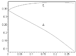
Figure 1: The mean fields $\Delta$ and $\xi$ versus the hole concentration $x$ in the uniform dRVB state. $t/J=3$.

Motivated by the approximate $4\times 4$ charge ordered states observed in STM experiments, we consider several types of parent patterns shown below with periodicity of $4a$ along both directions in the square lattice. Each symbol represents a lattice site, and the sites marked with the same symbol have the same electron density.

We denote $n_{\diamond}=n+\delta_{1}$, $n_{\circ}=n+\delta_{2}$, and $n_{\star}=n+\delta_{3}$. Since the overall average electron density of the system is $n$, only two out of the three $\delta^{\prime}s$ are independent. By using Eq. (4), we have $\bar{g}^{I}_{t,s}=\frac{1}{2}g_{t,s}^{\diamond\star}+\frac{1}{2}g_{t,s}^{\circ\star}$, $\bar{g}^{I\!I}_{t,s}=\frac{1}{4}g^{\diamond\star}_{t,s}+\frac{3}{4}g^{\circ\star}_{t,s}$, $\bar{g}^{I\!I\!I}_{t,s}=\frac{1}{4}g^{\star\star}_{t,s}+\frac{1}{4}g^{\circ\circ}_{t,s}+\frac{3}{8}g^{\star\circ}_{t,s}+\frac{1}{8}g^{\star\diamond}_{t,s}$, and $\bar{g}^{I\!V}_{t,s}=\frac{1}{4}g^{\star\star}_{t,s}+\frac{1}{8}{g^{\circ\circ}_{t,s}}+\frac{1}{8}g^{\star\diamond}_{t,s}+\frac{1}{8}{g^{\circ\diamond}_{t,s}}+\frac{3}{8}g^{\star\circ}_{t,s}$, here the superscript in $\bar{g}$ indicates the type of the parent pattern, and the superscript in $g$ refers to the two sites with the marked symbols. The Coulomb energy can be shown to be quadratic in $\delta^{\prime}s$, and they are given by, in unit of $e^{2}/\epsilon a$,

$$\Delta E^{I}_{c}=-4.039\delta_{1}^{2}-4.039\delta_{2}^{2}-4.847\delta_{1}\delta_{2}$$

$$\Delta E^{I\!I}_{c}=-1.497\delta_{1}^{2}-7.959\delta_{2}^{2}-3.468\delta_{1}\delta_{2}$$

$$\Delta E^{I\!I\!I}_{c}=-0.567\delta_{1}^{2}-3.772\delta_{2}^{2}-2.511\delta_{1}\delta_{2}$$

$$\Delta E^{I\!V}_{c}=-1.248\delta_{1}^{2}-4.138\delta_{2}^{2}-1.428\delta_{1}\delta_{2}.$$ (7)

Using these expressions, we have optimized the energy by varying parameters $\delta_{1}$ and $\delta_{2}$, and obtained charge ordered states with lower energies. These states are derivatives of the parent patterns under the consideration, but may have a higher symmetry than the parent state for those sites marked with different symbols may have the same electron density. Below we shall discuss our results in three different regions of the hole concentration. In all of our calculations, we use $J/t=1/3$, $t=0.3eV$, $a=3.8\AA$.

At the hole density around 1/16, the lower energy charge ordering pattern is $A1$ as shown in Fig.2. There are only two types of the distinct sites in terms of the electron density in this pattern. The numerical values of the energy gain and the charge distributions are given in Table 1 for $x=1/16$ and $x=0.05$. All other patterns at these dopings have energies either higher than or too close to the energy of the uniform dRVB state ($\Delta E>-0.01eV$), and are not listed here. At $x=1/16$, and $\epsilon=1$, the lowest energy state has a charge distribution slightly deviated from a commensurate state with the light site completely empty ($n=0$) and the dark site fully occupied ($n=1$). At a larger $\epsilon$, the energy gain decreases rapidly and the energy of the pattern $A1$ is just slightly lower than that of the homogenous case at $\epsilon=1.5$. There is no stable charge ordering pattern at $\epsilon$ much larger than $1.5$. $x=1/16$ is an ideal hole density for the pattern $A1$, which was also discussed in fu and suggested in the magnetic and optical measurements kim ; zhou . At $x=0.05$, the pattern $A1$ is stable only for smaller $\epsilon$, but is no longer stable for $\epsilon=1.5$. Note that the pattern $A1$ at $x=0.05$ is an insulator for there is no any connected path for holes to move through the lattice.

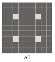
Figure 2: Low energy charge ordering pattern $A1$ of $4a\times 4a$ symmetry at hole density $x$ around 1/16. Shown are $9\times 9$ patches. Each square represents a lattice site and the light (dark) square represnts low (high) electron density.

Table 1: The energy and charge distribution of pattern $A1$ at hole density $x=0.0625$ and $x=0.05$. An ideal hole crystal state with $n_{{\color[rgb]{0.38,0.38,0.38}\scriptscriptstyle{\blacksquare}}}=1$ at $x=0.0625$ is also listed for comparison.

$x$	$0.0625$			$0.05$
$\epsilon$	$1$		$1.5$	$1$
$\Delta E$($eV$)	-0.038	-0.037	-0.010	-0.016
$n_{{\color[rgb]{0.85,0.85,0.85}\scriptscriptstyle{\blacksquare}}}$	0.005	0.000	0.017	0.200
$n_{{\color[rgb]{0.38,0.38,0.38}\scriptscriptstyle{\blacksquare}}}$	0.999	1.000	0.999	1.000
Pattern	A1	A1	A1	A1

Table 2: The energy and charge distribution of lower energy charge ordering patterns at hole density $x=0.125$ and $x=0.1$. The energies of some patterns with charge distribution of $n_{{\color[rgb]{0.38,0.38,0.38}\scriptscriptstyle{\blacksquare}}}=1$ are also listed for comparison.

$x$	$0.125$										$0.1$
$\epsilon$	$1$					$1.5$			$2$		$1$					$1.5$
$\Delta E$($eV$)	-0.116	-0.113	-0.056	-0.041	-0.013	-0.048	-0.043	-0.025	-0.015	-0.010	-0.059	-0.056	-0.051	-0.039	-0.021	-0.021	-0.017
$n_{\scriptscriptstyle\square}$			0.000	0.000				0.000		0.000			0.000	0.000	0.000	0.000
$n_{{\color[rgb]{0.85,0.85,0.85}\scriptscriptstyle\blacksquare}}$	0.006	0.000	0.875	0.857	0.542	0.018	0.000	0.898	0.042	0.909	0.208	0.200	0.933	0.914	0.925	0.943	0.230
$n_{{\color[rgb]{0.38,0.38,0.38}\scriptscriptstyle{\blacksquare}}}$	0.999	1.000	0.984	1.000	0.986	0.999	1.000	0.964	0.994	0.954	0.999	1.000	0.984	1.000	1.000	0.975	0.996
pattern	B1	B1	B2	B2	B3	B1	B1	B2	B1	B2	B1	B1	B2	B2	B4	B2	B1

Table 3: Energies and charge distributions of lower energy charge ordering patterns at $x=0.15$

$\epsilon$	$1$								$1.5$				$2$				$2.5$
$\Delta E$($eV$)	-0.129	-0.113	-0.113	-0.110	-0.093	-0.062	-0.044	-0.035	-0.063	-0.048	-0.046	-0.044	-0.029	-0.148	-0.011	-0.010	-0.010
$n_{\scriptscriptstyle\square}$		0.000	0.000	0.000	0.000	0.000	0.000			0.000	0.000	0.000		0.000	0.000	0.000
$n_{\scriptscriptstyle{\color[rgb]{0.85,0.85,0.85}\blacksquare}}$	0.000	0.933	0.950	0.950	0.933	0.828	0.800	0.428	0.000	0.950	0.933	0.950	0.000	0.950	0.933	0.950	0.000
$n_{{\color[rgb]{0.38,0.38,0.38}\scriptscriptstyle{\blacksquare}}}$	0.972	1.000	1.000	1.000	1.000	0.975	1.000	0.991	0.973	1.000	1.000	1.000	0.973	1.000	1.000	1.000	0.973
Pattern	B1	C1	C3	C2	C4	B2	B2	B3	B1	C3	C1	C2	B1	C3	C1	C2	B1

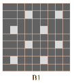
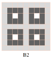
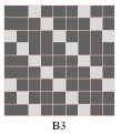
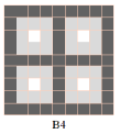
Figure 3: Lower energy charge ordering patterns for hole density around $x=1/8$. $B1$ is of a symmetry of $\sqrt{8}a\times\sqrt{8}a$, and $B3$ is a stripe.

At the hole density around $1/8$, there are several charge ordering patterns as shown in Fig.3. Among them the favorable pattern is $B1$. Patterns $B2$ and $B4$ have three types of distinct sites in terms of the electron density, while $B1$ and $B3$ have two types of distinct sites. The energy gain and the charge distribution are given in Table 2 for $x=1/8$ and $x=0.1$. Here we only list those patterns with relatively lower energies. As we can see from table 2, at $x=1/8$ the energies of patterns $B1$ and $B2$ are slightly lower than that of the homogeneous case at $\epsilon=2$. At $x=0.1$, the energy gain due to the charge ordering at $\epsilon=2$ is already very tiny.

It is interesting to note that around the low hole density $x=1/8$, both the checkerboard pattern $B2$ and the stripe patterntranquada $B3$ are SC states for holes in these patterns can move through the lattice.

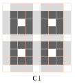
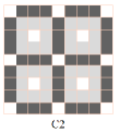
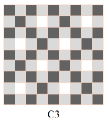
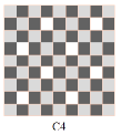
Figure 4: Several lower energy charge ordering patterns at $x=0.15$, not included in Figs 3. Patterns C1 and C2 are related by the interchange of the dark and gray sites, so for patterns C3 and C4.

At high hole concentrations, several new charge ordering patterns with lower energies appear, which are shown in Fig.4. In Table 3, we list the energies and charge densities of the lower energy patterns at $x=0.15$. For $\epsilon=1$, the five patterns ($B1$, $C1$, $C2$, $C3$, and $C4$) have very close energies. In the pattern C’s, the electron densities at the dark and grey sites are quite close. The empty sites in patterns $B1$ and C’s form a $\sqrt{8a}\times\sqrt{8a}$ Wigner hole crystal. Among the series C, pattern C1 is a conducting phase. We do not find any lower energy charge ordering pattern at $\epsilon>2.5$. At $x=0.2$, the most favroable patterns are $C1$, $C4$ and the stripe pattern $B3$.

In the energy estimation for the charge ordered RVB state, we have focused on the effect of the charge density dependent renormalization factors, but neglected the site-dependence of the mean fields $\xi$ and $\Delta$. This approximation turns out to be quite good in a limiting case where all the holes are completely localized at a single site. Consider pattern $A1$ at $x=1/16$ and pattern $B1$ at $x=1/8$ with the electron density $n$ either zero or 1. In this limit, the kinetic energy vanishes. The spin exchange energy of the state can be estimated by a direct counting of the missing bonds due to the vacancies in an otherwise half filled background, which is given by $E_{s}=2(1-2x)\alpha$ per site, with $\alpha=-0.344J$ the spin exchange energy per bond at the half filling. For $J=0.1eV$ we have $E_{s}=-0.060eV$ at $x=1/16$ and $E_{s}=-0.052eV$ at $x=1/8$, which are very close to the results obtained in the present MFT: $E_{s}=0.063eV$ at $x=1/16$ and $E_{s}=-0.054eV$ at $x=1/8$.

In summary we have studied the charge ordered RVB states in the doped cuprates within a generalized $t-J$ model by using a renormalized mean field theory. While the kinetic energy favors a uniform charge distribution, the long range Coulomb repulsion tends to spatially modulate the charge density in favor of charge ordered RVB states. Since both the Coulomb potential and the leading order in kinetic energy are quadratic in the density variation, we expect and indeed have found that the charge density variation from the uniform state is always large in the charge ordered state. The stability of the charge ordered RVB state strongly depends on the dielectric constant $\epsilon$. In cuprates, $\epsilon\approx 2.5-5$. Our calculation suggests that the observed charge ordered state in STM experiments in cuprates may well be interpreted due to the long range Coulomb interaction. Among the favorable charge ordered superconducting states, pattern $B1$ has a symmetry of $\sqrt{8}\times\sqrt{8}$, patterns $B2$ and $C1$ both have checkerboard structure, and pattern $B3$ is a stripe. Because of the intersite Coulomb repulsion, we do not find the bound hole paris in the charged ordered states.

The work is partially supported by NSFC No.10225419 and 90103022, and by RGC in Hong Kong, and by the US NSF ITR grant No. 0113574. One of us (FCZ) thanks P. W. Anderson for providing Ref. anderson prior to the publication.

References

- (1) J.E. Hoffman, et al., Science 295, 466 (2002).
- (2) C. Howald et al., Phys. Rev. B 67, 014533 (2003).
- (3) J.E. Hoffman, et al., Science 297, 1148 (2002).
- (4) K. McElroy et al., Nature 422, 520 (2003).
- (5) M. Vershinin et al, Science 303, 1995 (2004)
- (6) K. McElroy et al., to be published (2004).
- (7) T. Hanaguri et al., submitted to Nature.
- (8) M. Franz, D. E. Sheehy, and Z. Tesanovic, Phys. Rev. Lett. 88, 257005 (2002).
- (9) Q. Wang and D. H. Lee, Phys. Rev. B67, 020511 (2003).
- (10) H.D. Chen, O. Vafek, A. Yazdani, and S.C. Zhang, cond-mat/0402323.
- (11) H.C. Fu, J.C. Davis and D-H Lee, cond-mat/0403001.
- (12) P.W. Anderson, cond-mat/0406038.
- (13) R. Laughlin, LANL con-mat/0209269.
- (14) F. C. Zhang, Phys. Rev. Lett. 90, 207002 (2003).
- (15) F.C. Zhang, C. Gros, T.M. Rice and H. Shiba, J. Supercond. Sci. Tech.1, 36 (1988).
- (16) P. W. Anderson, P. A. Lee, M. Randerai, N. Trievedi, and F. C. Zhang, J. Phys.: Condensed Matter 24 R755, (2004).
- (17) M. C. Gutzwiller, Phys. Rev. 137, A1726 (1965).
- (18) D. Vollhardt, Rev. Mod. Phys. 56, 99 (1984).
- (19) Y. H. Kim and P. H. Hor, Mod. Phy. Lett. B15, 497 (2001); P. H. Hor and Y. H. Kim, J. Phys.: Condens. Matter 14, 10377 (2002).
- (20) F. Zhou et al., Supercon. Sci. Technol. 16, L7 (2003)
- (21) J.M. Tranquada et al, Nature 375, 561 (1995); J. Zaanen, O. Gunnarson, Phys. Rev. B. 40, 7391 (1989); V.J. Emery, S.A. Kivelson, Physica C 209, 597 (1993).