Now at]Department of Physics, University of Massachusetts, Amherst, MA 01003.

Interplay of instabilities in mounded surface growth

Abstract

We numerically study a one-dimensional conserved growth equation with competing linear (Ehrlich-Schwoebel) and nonlinear instabilities. As a control parameter is varied, this model exhibits a non-equilibrium phase transition between two mounded states, one of which exhibits slope selection and the other does not. The coarsening behavior of mounds in these two phases is studied in detail. In the absence of noise the steady-state configuration depends crucially on which of the two instabilities dominates the early time behavior.

The phenomenon of formation and coarsening of mounds in epitaxially grown thin films Krug:97 is a subject of much recent experimental Johnson:94 ; Apostolopoulos:00 and theoretical Siegert:94 ; Politi:96 ; Rost:97 interest. Traditionally, the formation of mounds has been attributed to the presence of an Ehrlich-Schwoebel (ES) step-edge barrier Ehrlich:96 ; Schwoebel:69 that hinders the downward motion of atoms across the edge of a step. This leads to an effective “uphill” surface current Villain:91 that has a destabilizing effect, leading to the formation of mounded structures. The ES mechanism is usually represented in continuum growth equations as a linear instability Villain:91 that is controlled by higher-order nonlinear terms. In ES-type models, the characteristics of the coarsening process, in which the typical lateral size of the mounds grows in time, depends on the details of the model. In these models, slope selection occurs (i.e. the slope of the mounds remains constant during coarsening) only if the “ES part” of the slope dependent surface current has one or more stable zeros as a function of the slope.

In our earlier work Chakrabarti:03 ; Chakrabarti:04 on a class of spatially discrete, conserved, one-dimensional (1d) models of epitaxial growth, we found a mechanism of mound formation and coarsening with slope selection that is different from the conventional ES mechanism. We studied the spatially discretized Lai-Das Sarma equation Lai:91 of MBE growth and an atomistic model Kim:94 that provides a discrete realization of the dynamics described by this equation, and found the occurrence of a nonlinear instability Dasgupta:97 in which isolated pillars or grooves grow in time if their height or depth exceeds a “critical” value. When this instability is controlled by the introduction of an infinite number of higher order gradient nonlinearities, these models show, for a range of parameter values, the formation of mounds with a well-defined slope that remains constant during the coarsening process. These results demonstrate that mound formation and power-law coarsening with slope selection can occur in the absence of an ES instability.

In most experimentally studied systems, however, it is believed that the ES step-edge barrier is present, although it may possibly be very weak. It is, therefore, important to understand how the behavior of our models would be modified when the ES mechanism is incorporated in their kinetics. To address this issue, we have studied, using numerical integration, a spatially discretized 1d growth equation in which a linear ES-type instability is present in conjunction with the nonlinear instability mentioned above. The main results of this study are as follows. Depending on the values of the parameters appearing in the model, we find two different mounded states. If the parameters are such that the nonlinear instability is the dominant one, then the behavior of the system is similar to that found in our earlier studies Chakrabarti:03 ; Chakrabarti:04 : it exhibits the formation of triangular mounds and power-law coarsening with slope selection. If, on the other hand, the linear instability is dominant, then the system exhibits a different kind of mounded state in which the mounds have a cusp-like shape and they steepen during the coarsening process. We call these two mounded states “faceted” and “cusped”, respectively. As the parameters are changed, the system undergoes a dynamical phase transition from one of these mounded states to the other.

We study a spatially discretized 1d version of the fourth order conserved growth equation, proposed in the context of MBE growth Lai:91 ; Villain:91 , in which the nonlinear instability Dasgupta:97 is controlled using a control function Chakrabarti:03 ; Chakrabarti:04 of the form proposed by Politi and Villain Politi:96 and a linear instability of the form proposed by Johnson et al. Johnson:94 to represent the ES effect is also included. Thus, the equation of motion of the interface height in appropriately non-dimensionalized form is written as:

$$\partial h_{i}/\partial t=-\tilde{\nabla}^{4}h_{i}+\lambda\tilde{\nabla}^{2}(|\tilde{\nabla}h_{i}|^{2}/(1+c_{1}|\tilde{\nabla}h_{i}|^{2}))-$$

$$\tilde{\nabla}(\tilde{\nabla}h_{i}/(1+c_{2}|\tilde{\nabla}h_{i}|^{2}))+\eta_{i}(t),$$ (1)

where $h_{i}$ is the non-dimensionalized height variable at lattice site $i$, and $\tilde{\nabla}$ and $\tilde{\nabla^{2}}$ are the lattice versions of the derivative and Laplacian operators, respectively, calculated using the nearest neighbors as outlined in our earlier papersChakrabarti:03 ; Chakrabarti:04 . In Eq.(1), $c_{1}$, $c_{2}$ and $\lambda$ are constants (model parameters), and $\eta_{i}(t)$ represents uncorrelated random noise with zero mean and unit variance. Our results are based on numerical integration of this equation in 1d, using a simple Euler schemeDasgupta:97 in which the time evolution of the height variables is given by

$$h_{i}(t+\Delta t)=h_{i}(t)+\Delta t\{\tilde{\nabla}^{2}[-\tilde{\nabla}^{2}h_{i}(t)+$$

$$\lambda(|\tilde{\nabla}h_{i}(t)|^{2}/(1+c_{1}|\tilde{\nabla}h_{i}(t)|^{2}))]-$$

$$\tilde{\nabla}(\tilde{\nabla}h_{i}(t)/(1+c_{2}|\tilde{\nabla}h_{i}(t)|^{2}))\}+\sqrt{\Delta t}\,\eta_{i}(t).$$ (2)

In all our calculations, the value of the parameter $c_{2}$ was held fixed at unity, and $c_{1}$ and $\lambda$ were varied. Our results are obtained for different system sizes, $40\leq L\leq 1000$, with periodic boundary conditions. We do not find any significant $L$-dependence. We have used a time step $\Delta t$=$0.01$ for most of our studies and checked that very similar results are obtained with smaller values of $\Delta t$. The results obtained by using a more sophisticated algorithm Shampine:94 closely match with those of our Euler scheme for a small enough $\Delta t$. We have also checked that the basic features of our results remain unaltered if other boundary conditions (such as “fixed” and “zero-flux” boundary conditions considered in our earlier work Chakrabarti:03 ; Chakrabarti:04 ) are used.

We first describe the results obtained in the absence of the noise term. In this case, we find that if the parameter $c_{1}$ is sufficiently small, then the long time behavior of the interface depends on which of the instabilities dominates at early times. In order to characterize this, we considered initial configurations with a single pillar of height $h_{0}$ on an otherwise flat interface, and studied the long-time behavior as a function of $h_{0}$. We find that when $h_{0}$ is sufficiently small, so that the nonlinear instability is not initiated, the linear instability dominates the time evolution and the resulting morphology is mounded without slope selection. If on the other hand $h_{0}$ is large enough to seed the nonlinear instability, then mounds with a “magic” slope result. This is illustrated in Fig. 1 which shows typical configurations obtained in the two cases: slope selected mounds (“faceted”) in situations where the height of the central pillar is greater than a critical value and mounds without slope selection (“cusp” like ) otherwise. Fig. 1 also shows the dependence of the critical value of $h_{0}$ on $\lambda$, the strength of the nonlinearity. We find that this critical value is approximately given by $A/\lambda$, $A\simeq 21$, with a weak dependence on the parameter $c_{1}$.

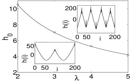
Figure 1: Dependence of the morphology on the initial conditions in the absence of noise. Main plot: the critical value of $h_{0}$ (see text) as a function of the nonlinearity parameter $\lambda$ for $c_{1}=0.01$. This critical value is approximately given by $h_{0}=21/\lambda$ (solid line). Upper inset: “faceted” morphology for $h>h_{0}$. Lower inset: “cusped” morphology for $h<h_{0}$.

This “bistable” behavior is found only if the control parameter $c_{1}$ is sufficiently small. Otherwise, the system evolves to the cusped morphology even if the initial configuration has a high central pillar. Thus, the faceted morphology is found in the zero-noise simulations only if $c_{1}<c_{1}^{sp}(\lambda)$ (the superscript $sp$ denotes “spinodal”, see below) and the initial configuration is sufficiently rough to seed the nonlinear instability. This behavior may be understood from a linear stability analysis. In both faceted and cusped growths, the finite-sized system evolves, at long times, to a profile with a single mound which is a fixed point of the noiseless dynamics. Examples of such profiles (obtained from simulations with noise which slightly roughens the profiles) are shown in Figs. 2 and 3. These fixed points can also be obtained by calculating the $h_{i}$ for which $g_{i}$=0 for all $i$, where $g_{i}$ is the term multiplying $\Delta t$ on the right-hand side of Eq.(2). The local stability of the faceted fixed point may be determined from a calculation of the eigenvalues of the matrix $M_{ij}=\partial g_{i}/\partial h_{j}$ evaluated at the fixed point. We find that the largest eigenvalue of this matrix crosses zero at a “spinodal” value, $c_{1}=c^{sp}_{1}(\lambda)$ (see inset of Fig. 6), signaling an instability of the faceted profile. Thus, for $0<c_{1}<c^{sp}_{1}(\lambda)$, the dynamics of Eq.(2) without noise admits two locally stable invariant profiles: a cusped profile without slope selection, and a faceted one with slope selection. Depending on the initial state, the no-noise dynamics takes the system to one of these two fixed points. For example, an initial state with one pillar on a flat background is driven by the no-noise dynamics to the cusped fixed point if the height of the pillar is smaller than a critical value (mentioned earlier), and to the faceted one otherwise. The dependence of $c^{sp}_{1}$ on the nonlinearity parameter $\lambda$ is shown in Fig. 6. Such a “spinodal line” does not exist for the cusped fixed point.

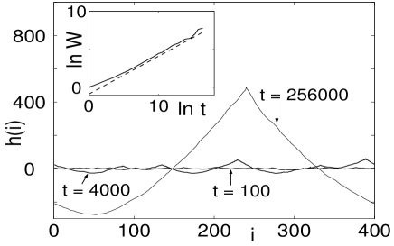
Figure 2: The interface profiles at three different times ($t$= 100, 4000 and 256000) in a run with noise starting from a flat state for an $L=400$ sample with $\lambda=4.0$ and $c_{1}=0.05$. A double log plot of the interface width $W$ as a function of time $t$, averaged over $15$ runs for $L=1000$ samples in the presence of noise, and a power-law fit are shown in the inset.

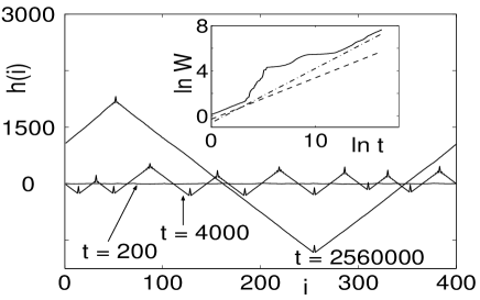
Figure 3: Interface profiles at three different times ($t$= 200, 4000 and 2560000) in a run starting from a flat state for an $L=400$ sample with $\lambda=4.0$ and $c_{1}=0.01$. A double log plot of the interface width $W$ as a function of time $t$, averaged over $15$ runs for $L=1000$ samples in the presence of noise, and power-law fits to the early and late-time data are shown in the inset.

We have studied in detail the process of coarsening of the mounds in the two different (faceted and cusped) growth modes. In these simulations, the initial configuration is obtained by setting $h_{i}=h_{0}r_{i}$ where $r_{i}$ is a random number uniformly distributed between $-1$ and $1$. If $c_{1}<c_{1}^{sp}$ and $h_{0}$ is sufficiently large to initiate the nonlinear instability, the system evolves to a faceted structure; a cusped structure is obtained otherwise. The results reported here were obtained from averages over 20 such runs with different initial configurations. In the region of parameter space, $0<c<c^{sp}_{1}(\lambda)$, where the faceted phase is locally stable, the mounds coarsen in time with the slope of the mounds remaining constant. In this case, the average mound size $R(t)$ is obviously proportional to the interface width $W(t)$. As shown in Fig 4, the interface width in this growth mode increases as a power-law with time in the long-time coarsening regime, while the slope of the mounds remains constant in time. The exponent $\beta$ that described this power-law coarsening behavior, $W(t)\propto R(t)\propto t^{\beta}$, is found to be close to 0.5. The coarsening of mounds in the cusped regime (i.e. for $c_{1}>c^{sp}_{1}(\lambda)$ and any initial configuration, and $c_{1}<c^{sp}_{1}(\lambda)$ and sufficiently smooth initial configurations) is qualitatively different. In this growth mode, both the interface width and the average slope $s(t)$ of the cusp-like mounds (as well as the maximum slope $s_{m}(t)$) increases with time as a power law in the coarsening regime: $W(t)\propto t^{\beta}$, and $s(t)\propto t^{\theta}$. This implies that the average mound size also increases with time as a power law: $R(t)\propto t^{n}$ with $n=\beta-\theta$. This behavior is illustrated in Fig. 5. The values of the exponents are found to be $\beta=0.54\pm 0.02$ and $\theta=0.2\pm 0.02$, implying that the coarsening exponent is $n=0.34\pm 0.04$.

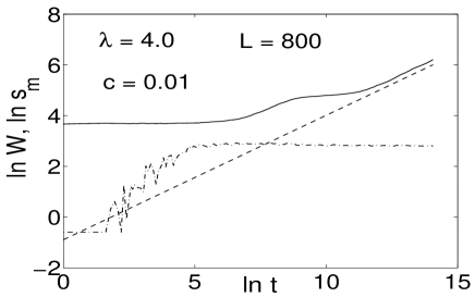
Figure 4: Double log plots of the width $W$ (full line) and the average of the maximum slope $s_{m}$ (dash-dotted line) as a function of time $t$, for faceted growth with slope selection in the absence of noise. This data are for $\lambda=4.0$, $c_{1}=0.01$, and $L=800$, averaged over $20$ initial conditions. In this case the growth exponent $\beta=0.5\pm 0.01$ (the dashed line is the best power-law fit) and the steepening exponent $\theta=0$.

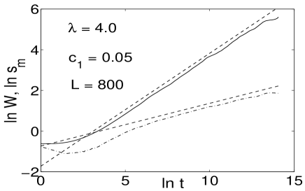
Figure 5: Variation of width $W$ (full line) and the average of the maximum slope, $s_{m}$ (dash-dotted line) as a function of time $t$ on a log-log scale for cusped growth in the absence of noise ($\lambda=4.0$, $c_{1}=0.05$, and $L=800$ averaged over $20$ initial conditions). The growth exponent is $\beta=0.54\pm 0.02$, and the steepening exponent $\theta=0.2\pm 0.02$. Best power-law fits are shown by the dashed lines.

In the presence of noise, the steady state behavior is independent of the initial condition. When the control parameter $c_{1}$ is sufficiently large, the nonlinear instability is completely suppressed and the route to mounding is similar to the linear instability dominated behavior mentioned above, the configurations being slightly roughened versions of their noiseless counterpart. This is illustrated in Fig. 2 where the interface profiles in a typical run starting from a flat state for $L=400$, $\lambda=4.0$ and $c_{1}=0.05$ are shown at times $t=100$ (early time regime), $t=4000$ (coarsening regime) and $t=256000$ (steady state). The inset shows the interface width $W$ as a function of $t$, averaged over $15$ runs for $L=1000$ samples. The averaged data show $W\propto t^{\beta}$, $\beta=0.5\pm 0.01$ in the coarsening regime. The average slope of the mounded interface grows as $s(t)\propto t^{\theta}$, with $\theta=0.18\pm 0.02$ and hence the coarsening exponent is $n=0.32\pm 0.03$.

As the value of $c_{1}$ is decreased below a critical value holding $\lambda$ fixed, the nonlinear instability dominates over the linear one. At early times in runs starting from a flat state, the interface is self affine and the interface width shows power law scaling with an exponent close to 0.37. As time progresses isolated pillars with height $h_{0}>h_{min}$, where $h_{min}$ is the minimum height of such a pillar above which the nonlinear instability is operative, make their appearance through random fluctuations. The time evolution of the interface beyond the point of occurrence of the instability is similar to that in the noiseless situation. In Fig. 3 we present snapshots of an $L=400$ sample for $\lambda=4.0$ and $c_{1}=0.01$ at different stages of growth: $t=200$ (before the onset of the instability), $t=4000$ (coarsening regime), and $t=2560000$ (steady state). The inset shows a plot of the interface width as a function of time, obtained by averaging over $15$ runs for $L=1000$ samples. The averaged data show a power-law growth regime with exponent $0.37\pm 0.01$ before the onset of the instability and a second power-law coarsening regime with $W\propto t^{\beta}$, $\beta=0.49\pm 0.02$.

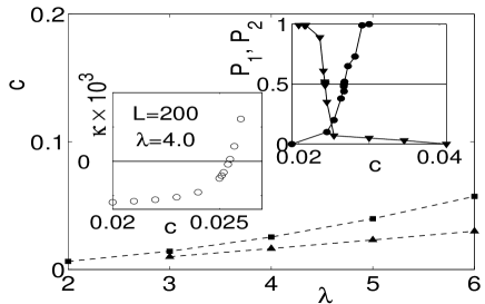
Figure 6: Phase diagram for a $L$= 200 system, where the critical values of the control parameter $c_{1}$ are shown as functions of $\lambda$. The critical value $c_{1}^{sp}$ ($c_{1}^{cr}$) above which the faceted phase is unstable (metastable) is shown by squares (triangles). The dashed lines are guides to the eye. Left Inset: Zero crossing of the largest eigenvalue $\kappa$ of the stability matrix of the faceted fixed point as a function of $c_{1}$ ($\lambda=4.0$, $L$ = 200). Right Inset: The probabilities $P_{1}$ (circles) and $P_{2}$ (inverted triangles) (see text) as functions of $c_{1}$ with $\lambda=5.0$ and $L$= 200.

A dynamical phase transition at $c_{1}=c^{cr}_{1}(\lambda)<c^{sp}_{1}(\lambda)$ separates these two kinds of growth modes. To calculate $c^{cr}_{1}(\lambda)$, we start a system at the faceted fixed point and follow its evolution according to Eq.(2) for a long time (typically $t=10^{4}$) to check whether it reaches a cusped steady state. By repeating this procedure many times (typically $100$ runs), the probability, $P_{1}(\lambda,c_{1})$, of a transition to a cusped state is obtained. For fixed $\lambda$, $P_{1}$ increases rapidly from 0 to 1 as $c_{1}$ is increased above a critical value. Typical results for $P_{1}$ as a function of $c_{1}$ for $\lambda=5.0$ are shown in the right inset of Fig. 6. The value of $c_{1}$ at which $P_{1}=0.5$ provides an estimate of $c^{cr}_{1}$. Another estimate is obtained from a similar calculation of $P_{2}(\lambda,c_{1})$, the probability that a flat initial state evolves to a faceted steady state. As expected, $P_{2}$ increases sharply from 0 to 1 as $c_{1}$ is decreased (see right inset of Fig. 6), and the value of $c_{1}$ at which this probability is 0.5 is slightly lower than the value at which $P_{1}=0.5$. This difference reflects finite-time hysteresis effects. The value of $c^{cr}_{1}$ is taken to be the average of these two estimates, and the difference between the two estimates provides a measure of the uncertainty in the determination of $c^{cr}_{1}$. The phase boundary obtained this way is shown in Fig. 6, along with the results for $c^{sp}_{1}$.

The scaling behavior in the coarsening regime in the presence of noise is the same as that found in the noiseless case. The qualitative behavior in the faceted phase is similar to that found in our earlier work Chakrabarti:03 ; Chakrabarti:04 on this model without the ES term. The ES term, however, has an important effect: it changes the coarsening exponent from 0.33 to 0.5. A model very similar to the one considered here was studied by Torcini and Politi Torcini:02 for parameter values deep in the cusped regime (small $\lambda$, large $c_{1}$). The mounded morphology we find in this regime is similar to that found in their study. Our results for the exponents $\theta$ and $n$ are slightly different from the values ($\theta=n=1/4$) reported by them. This is probably due to crossover effects – we have found values of $n$ closer to 1/4 if smaller values of $\lambda$ and/or larger values of $c_{1}$ are used.

In summary we have shown that a nonlinear instability in our spatially discrete growth model in which the linear ES instability is also present may, for appropriate parameter values, lead to mound formation with slope selection and power-law coarsening. This is qualitatively different from the behavior in the parameter regime where the ES instability dominates: the system exhibits mound formation in this regime also, but there is no slope selection. The coarsening exponent has different values in these two regimes which are separated by a line of first-order dynamical phase transitions. The ES part of the surface current in our model does not vanish for any non-zero value of the slope. Therefore, the slope selection we find in the regime where the nonlinear instability is dominant is qualitatively different from that in ES-type models and is a true example of nonlinear pattern formation. The noiseless version of our model exhibits an interesting dependence on initial conditions: the long-time behavior depends on whether the inhomogeneities in the initial configuration are sufficient to seed the nonlinear instability. Both kinds of mounding behavior found in this study have been observed in experiments, and our model may be relevant in the development of an understanding of these experimental observations. However, more work is required to establish a connection between our results and those of experiments.

References

- (1) J. Krug, Adv. Phys. 46, 139 (1997).
- (2) M. D. Johnson, C. Orme, A. W. Hunt, D. Graff, J. Sudijono, L. M. Sander and B. G. Orr, Phys. Rev. Lett 72, 116 (1994).
- (3) G. Apostolopoulos, J. Herfort, L. Daweritz and K. H. Ploog, Phys. Rev. Lett. 84, 3358 (2000), and references therein.
- (4) M. Siegert and M. Plischke, Phys. Rev. Lett. 73, 1517 (1994).
- (5) P. Politi and J. Villain, Phys. Rev. B 54, 5114 (1996).
- (6) M. Rost and J. Krug, Phys. Rev. E 55, 3952 (1997), and references therein.
- (7) G. Ehrlich and F. G. Hudda, J. Chem. Phys. 44, 1039 (1996).
- (8) R. L. Schwoebel, J. Appl. Phys. 40, 614 (1969).
- (9) J. Villain, J. Phys. I (France) 1, 19 (1991).
- (10) B. Chakrabarti and C. Dasgupta, Europhys. Lett. 61, 547 (2003).
- (11) B. Chakrabarti, and C. Dasgupta, Phys. Rev. E 69, 011601 (2004).
- (12) Z. W. Lai, and S. Das Sarma, Phys. Rev. Lett. 66, 2348 (1991).
- (13) J. M. Kim and S. Das Sarma, Phys. Rev. Lett. 72, 2903 (1994).
- (14) C. Dasgupta, J. M. Kim, M. Dutta, and S. Das Sarma, Phys. Rev. E 55, 2235 (1997).
- (15) L. F. Shampine, Numerical Solution of Ordinary Differential Equations (Chapman & Hall, New York, 1994).
- (16) A. Torcini, and P. Politi, Eur. Phys. J. B 25, 519, (2002).