Tunneling in a uniform one-dimensional superfluid: emergence of a complex instanton

Abstract

In a uniform ring-shaped one-dimensional superfluid, quantum fluctuations that unwind the order parameter need to transfer momentum to quasiparticles (phonons). We present a detailed calculation of the leading exponential factor governing the rate of such phonon-assisted tunneling in a weakly-coupled Bose gas at a low temperature $T$. We also estimate the preexponent. We find that for small superfluid velocities the $T$-dependence of the rate is given mainly by $\exp(-c_{s}P/2T)$, where $P$ is the momentum transfer, and $c_{s}$ is the phonon speed. At low $T$, this represents a strong suppression of the rate, compared to the non-uniform case. As a part of our calculation, we identify a complex instanton, whose analytical continuation to suitable real-time segments is real and describes formation and decay of coherent quasiparticle states with nonzero total momenta.

I Introduction

Many one-dimensional (1D) systems share a universal low-energy description based on a complex order parameter Haldane . Probably the most familiar example is a superfluid confined to a narrow channel, but—due to the well-known “duality” between bosons and fermions in one dimension—a similar description exists also for fermionic fluids.

In accordance with the Bogoliubov-Hohenberg theorem, no long-range order is possible in these 1D systems, but the precise nature of fluctuations that prevent ordering deserves a further discussion. At zero temperature ($T=0$), perturbative fluctuations of the phase of the order parameter (phonons in a superfluid) cause a power-law decay of spatial correlations. At $T\neq 0$, the decay becomes exponential. However, a detailed study Haldane of the $T=0$ case reveals additional contributions to the correlation functions, of the form of a power law multiplied by an oscillating factor.

While for weakly-coupled Fermi systems these oscillating terms can be seen as a 1D version of Friedel oscillations, for weakly-interacting bosons their interpretation is not immediately obvious. It is possible, however, to interpret them as a consequence of nonperturbative fluctuations: instantons or quantum phase slips (QPS). The oscillatory dependence on the spatial coordinate can be traced to the fact (readily verified, see below) that each QPS changes the linear momentum of the superfluid component.

The momentum production by QPS results from unwinding the order parameter and the corresponding change in the supercurrent. More formally, it can be viewed as a consequence of a special type of topological term, present in the action of a 1D weakly-coupled Bose gas. We discuss this term in detail in the next section.

A complementary picture is obtained by looking at the Lieb-Liniger spectrum Lieb&Liniger (for a gas with a delta-function repulsion). Their results apply for periodic boundary conditions, i.e., ring geometry, which is the only case we consider here. In the limit $L\to\infty$, where $L$ is the length of the ring, the spectral branch associated with solitons solitons touches zero at momentum $P=2\pi n$, where $n$ is the gas density. This state corresponds precisely to the order parameter winding once as we go around the ring. Phonon-assisted transitions to this state will destroy superfluidity. Our aim will be to calculate the rate of such transitions at low temperatures.

Except for a brief summary in Sect. III of results for QPS induced by a localized perturbation, we consider here only uniform 1D superfluids. In the ring geometry, momentum in the longitudinal ($x$) direction is conserved. (More precisely, we should be talking about angular momentum, but this distinction will not be important for our purposes.) Our goal was to see how momentum conservation influences the QPS rate. Some results of this work have been presented in ref. slip . Here we describe a different, more systematic method, which confirms the results of slip , but also allows us to obtain new results.

At $T=0$, the 1D gas can be mapped on a two-dimensional (2D) model by introducing the imaginary (Euclidean) time $\tau$. QPS are vortices—or instantons—of this 2D model. Although this model is similar to the usual XY model, the topological term drives it into a different universality class. The XY model, as the coupling is increased, undergoes a Berezinsky-Kosterlitz-Thouless (BKT) transition. In contrast, in the Bose gas, the correlation functions Haldane evolve continuously. We show in Sect. III that, for a weakly-coupled uniform Bose gas at zero temperature, instantons and antiinstantons are bound in pairs by a linear, rather than logarithmic, potential. An extrapolation of this result to strong coupling implies that the breaking of instanton pairs, characteristic of a BKT transition, is not possible, a conclusion consistent with the expected Galilean invariance of the $T=0$ state.

Instanton-antiinstanton pairs can unbind if there is an additional source of energy, besides the energy resulting from unwinding the supercurrent. This possibility may be of interest for analog models of gravity Unruh ; Garay&al . It has been suggested that one can use cold Bose gases to model cosmologically interesting spacetimes Fedichev&al ; Barcelo&al . If one models an expanding spacetime by varying (decreasing) the coupling $g$ between the atoms, as proposed in ref. Barcelo&al , then some of the energy supplied by this variation may become available for enhancement of QPS. We note also that a decrease in $g$ causes the principal length scale of the gas—the “healing” length $\xi$—to grow. Since the cross-sectional radius $R$ of the channel is fixed, the 1D regime $\xi>R$ can be reached.

Another possibility, which is the main subject of this paper, is when the additional source of energy is a low but nonzero temperature. We discuss this case in detail in Sect. IV. Thermally activated phase slips (TAPS) in the ring geometry have been considered, in the framework of the nucleation theory of Refs. Little ; LA ; McCH , in ref. TAPS . In the present paper, we concentrate on lower temperatures where, as we will see, the main mechanism for phase slips is thermally assisted quantum tunneling, rather than the over-barrier activation. One should note, however, that in the case of a uniform Bose gas, even at higher temperatures, the original LAMH theory LA ; McCH probably needs to be modified, in order to account for momentum conservation. We discuss this point further in the conclusion.

If the gas is uniform (or nearly uniform—the confining potential is smooth on the scale $\xi$, and its variations are small), QPS have a rather distinctive experimental signature. Indeed, as we will see, unwinding momentum $P$ from the supercurrent in such a uniform system is accompanied by transferring a compensating momentum to the phonon “bath”. This is equivalent to creating a flow of excited atoms, which can in principle be detected experimentally. For example, we can start with a state with no supercurrent and let a QPS create a unit of supercurrent and a compensating normal flow in the opposite direction (counterflow). The counterflow can be detected by the standard momentum imaging, i.e., opening the trap in one place. Note that no counterflow is expected for QPS induced by a highly localized perturbation, which breaks both momentum conservation and the Galilean invariance (calculation of the rate for this case has been done in ref. Kagan&al ). In that case, the final state of phonons has zero total momentum.

However, perhaps the most immediate experimental consequence of the momentum balance during QPS in a uniform system is that it leads to a strong suppression of the rate, compared to the case of a localized perturbation slip . The reason is that the momentum released by unwinding the supercurrent can only be absorbed by relatively high-energy phonons states, which are scarcely populated at a low temperature.

From the theoretical perspective, one would like to understand in general how to compute the rates of instanton processes that transfer momentum between the background and excitations. The question is not limited to QPS in narrow superfluid channels but arises also in other contexts. For example, one can view the momentum transfer by QPS as a 1D analog of the Magnus force in higher dimensions. This force acts on vortices moving in a superfluid and is known to suppress vortex tunneling Volovik . It is natural to ask if the suppression can be circumvented by an inelastic process similar to the one we consider here. Furthermore, additional interesting physics slip emerges in cases when the order parameter is coupled to fermions, as in the case of BCS superconductors. The coupling to fermions opens a new channel of momentum production, due to the fermion zero modes at the instanton core. This channel is a 1D analog of “momentogenesis” momen by vortices in 2D arrays of Josephson junctions. Although in the case of 1D superconductors the relevance of this channel is somewhat obscured by scattering of quasiparticles on the boundaries and disorder, it may still be of interest for interpretation of experiments exp1 ; exp2 on superconducting nanowires.

A much studied example of inelastic tunneling in field theory is instanton-induced scattering in gauge theories and their low-dimensional analogs instantons . Indeed, the complex instanton that we will find in this paper is a generalization of the (real) periodic instantons periodic to the case when there is nontrivial momentum transfer from the background to quasiparticles.

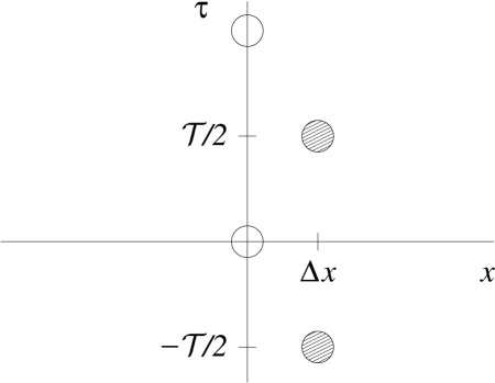
Figure 1: A periodic configuration, in which instantons (open circles) and antiinstantons (shaded circles) are shifted relative to each other in space by $\Delta x$. At a finite temperature $T$, the period of the configuration is ${\cal T}=\beta=1/T$.

In ref. slip , we have identified periodic Euclidean configurations (of period $\beta=1/T$, where $T$ is the temperature), which consist of chains of instantons and antiinstantons shifted relative to each other by amount $\beta/2$ in the imaginary time and by some $\Delta x$ in space, see Fig. 1. The tunneling rate has been obtained by integrating over $\Delta x$. Unlike the case without momentum transfer periodic , this integration is nontrivial. Nevertheless, the leading exponential factor obtained in this way has a simple physical interpretation. It can be interpreted as the rate of tunneling between quasiparticle (phonon) states with momenta $-P/2$ and $P/2$, so that the change in the momentum of phonons precisely compensates the momentum produced by unwinding the supercurrent.

In the present paper, we derive this leading result for the tunneling exponent, and the first correction to it, in what we regard as a more systematic way. First, using a method developed in ref. periodic , we obtain the tunneling exponent for a microcanonical state (fixed energy $E$). Then, we integrate the microcanonical rate over $E$ with the Boltzmann factor $\exp(-E/T)$ to obtain the canonical (fixed $T$) rate. This method allows us to find directly the energies corresponding to the dominant phase-slip paths. In particular, we can show that at sufficiently low $T$ thermally-assisted tunneling (as opposed to over-barrier activation) is indeed the dominant phase-slip mechanism.

We also discuss in detail the instanton solution that saturates the rate at nonzero momentum transfer $P$. This instanton corresponds to a complex saddle point for $\Delta x$ and is itself complex. Unlike the periodic instanton of ref. periodic , it has no turning points. Nevertheless, it is possible to identify the initial and final states connected by this complex instanton and to reconstruct their real-time evolution. On the real-time segments, the solution is real and can be interpreted as formation and decay of coherent phonon states corresponding to the tunneling endpoints. A direct computation confirms that the total momenta of these states are $-P/2$ and $P/2$.

II The topological term

A weakly-coupled 1D Bose gas can be described by the Gross-Pitaevsky (GP) Lagrangian, which in the Euclidean signature reads

$$L_{E}=\psi^{\dagger}\partial_{\tau}\psi+\frac{1}{2m}|\partial_{x}\psi|^{2}+{g\over 2}|\psi|^{4}-\mu|\psi|^{2}\;.$$ (1)

Here $\tau=it$ is the Euclidean time, $m$ is the mass of the particles, $g>0$ is the coupling constant, and $\mu$ is the chemical potential. We assume that the system is subject to periodic boundary conditions in the $x$ direction: $\psi(x+L)=\psi(x)$.

Instantons are vortices of this theory in the $(x,\tau)$ plane, corresponding to nontrivial winding of the phase of the order parameter $\psi$.

The number density of the gas is $\hat{n}=\psi^{\dagger}\psi$ and can be written as a sum of the average density $n$ and a fluctuation $\delta n$: $\hat{n}(x,t)=n+\delta n(x,t)$. We consider the uniform case, when $n$ (the average) is independent of $x$, but will comment briefly on the effect of nonuniform $n$, such as resulting from a confining potential.

At large wavelengths, fluctuations of the density are small, so $\psi$ has well-defined modulus and phase. We write $\psi=(n+\delta n)^{1/2}\exp(i\theta)$ and, expanding in small $\delta n$, obtain

$$L_{E}\approx i(n+\delta n)\partial_{\tau}\theta+{n\over 2m}(\partial_{x}\theta)^{2}+{g\over 2}(\delta n)^{2}\;.$$ (2)

Note that we impose no restrictions on the size of fluctuations of $\theta$, in accordance with the absence of long-range order. Note also that in (2) we have omitted a term containing gradients of $\delta n$. This is correct in the leading longwave approximation, but at shorter wavelengths that term will convert the purely acoustic dispersion law into the full dispersion of Bogoliubov’s quasiparticles Bogoliubov .

The approximation (2) applies away from the instanton core, but not at the core itself. This is because the size of the core is determined by the healing length

$$\xi=(4gmn)^{-1/2}\;,$$ (3)

while the long-wavelength approximation corresponds to wavenumbers $k\ll\xi^{-1}$ and so does not resolve the core.

In this approximation, the density fluctuations are Gaussian, and can be integrated out in the path integral. This amounts to using the equation of motion for $\delta n$ and substituting the result, $\delta n=-(i/g)\partial_{\tau}\theta$, back into eq. (2). In this way, we obtain a phase-only theory with the Euclidean Lagrangian

$$L_{E}\approx in\partial_{\tau}\theta+{1\over 2g}(\partial_{\tau}\theta)^{2}+{n\over 2m}(\partial_{x}\theta)^{2}\;.$$ (4)

Instantons are singular solutions of this theory. The presence of such singular solutions means that, even though the Lagrangian (4) is quadratic in $\theta$, the theory remains non-Gaussian.

From eq. (4), we can read off the speed of Bogoliubov’s phonons. We use units in which this speed is equal to 1:

$$c_{s}=(gn/m)^{1/2}=1\;.$$ (5)

In these units, eq. (3) takes the form

$$\xi=(2gn)^{-1}\;.$$ (6)

If it were not for the first term, the Lagrangian (4) would be that of the usual XY model. In that theory, individual QPS can occur at $T=0$ in any current-carrying state, due to the energy released by unwinding the supercurrent. This applies regardless of the strength of the coupling $g$. Moreover, at a sufficiently strong coupling (which is outside the domain of our semiclassical method) instanton-antiinstanton (IA) pairs unbind even in vacuum, resulting in a BKT phase transition.

However, the first term in (4) drastically modifies the properties of the theory. We refer to this term as topological. It is of the same nature as the topological contribution Magnus to the Magnus force acting on vortices in higher dimensionalities (2D and 3D). As we will now see, in 1D, for Euclidean paths that contain instantons, the topological term gives a nonzero contribution to the Euclidean action. Being purely imaginary, that contribution can be interpreted as the interference phase between QPS at different locations.

The simplest case when the the topological term can be seen to play a role is a single IA pair, with instanton located at $x^{\mu}_{0}=(x_{0},\tau_{0})$ and antiinstanton at ${x^{\mu}_{0}}^{\prime}=(x^{\prime}_{0},\tau^{\prime}_{0})$. Away from the cores, the density is approximately $n$, and the phase, in the absence of supercurrent, is

$$\theta_{\rm pair}(x,\tau)=\arg[x-x_{0}+i(\tau-\tau_{0})]-(x^{\mu}_{0}\leftrightarrow{x^{\mu}_{0}}^{\prime})\;.$$ (7)

For periodic boundary conditions, this is an approximation, which applies when all of the distances involved: $|x^{\mu}-x^{\mu}_{0}|$, $|x^{\mu}-{x^{\mu}_{0}}^{\prime}|$, and $|x^{\mu}_{0}-{x^{\mu}_{0}}^{\prime}|$, are much smaller than the length $L$ of the system.

The time derivative of the configuration (7) is

$$\partial_{\tau}\theta_{\rm pair}=\frac{x-x_{0}}{(x-x_{0})^{2}+(\tau-\tau_{0})^{2}}-(x^{\mu}_{0}\leftrightarrow{x^{\mu}_{0}}^{\prime})\;.$$ (8)

Integrating over $\tau$ and $x$, we obtain the topological action:

$$\Delta S_{\rm pair}=-2\pi in(x_{0}-x^{\prime}_{0})\;.$$ (9)

Since the variable conjugate to the position is momentum, we can interpret the action (9) as resulting from production of momentum

$$P=2\pi n\;,$$ (10)

by the antiinstanton and its absorption by the instanton.

The above interpretation is of course nothing new and is readily confirmed by a direct calculation. Noether’s momentum following from the real-time version of eq. (1) is

$$P=-i\int dx\psi^{\dagger}\partial_{x}\psi\;.$$ (11)

The difference between the initial and final momenta can be written as an integral over a large closed contour in the $(x,\tau)$ plane:

$$P_{\rm fin}-P_{\rm ini}=-i\oint_{C}d{\bf l}\cdot\psi^{\dagger}\nabla\psi\;,$$ (12)

where $C$ runs clockwise. If the contour encloses a single instanton, without any phonon excitations, then away from the core the density is $n$, and (12) equals precisely $-2\pi n$.

III QPS rate at $T=0$

In general, the metastable states connected by the instanton are current-carrying, which implies that the phase $\theta$ winds an integer number $N$ times over the length $L$ of the system. A suitable generalization of (7) is then

$$\theta_{c}(x,\tau)=\theta_{\rm pair}(x,\tau)+\frac{2\pi}{L}Nx\;.$$ (13)

The second, winding, term corresponds to superfluid velocity

$$V=\frac{2\pi N}{mL}\;.$$ (14)

In what follows, we will always assume that $V$ is much smaller than the speed of sound $c_{s}=1$ (although the more general case can be considered by similar methods). For $V\ll 1$, the field of the IA pair is only weakly affected by the superflow, and we can continue to use expression (7). However, the presence superflow leads to an additional contribution to the action. To logarithmic accuracy, we obtain

$$S_{\rm pair}=-iP\Delta x+E\Delta\tau+\frac{2\pi}{g}\ln\frac{d}{\xi}+O\left(\frac{1}{g}\right)\;,$$ (15)

where $\Delta x=x_{0}-x^{\prime}_{0}$, $\Delta\tau=\tau_{0}-\tau^{\prime}_{0}$, $d=(\Delta x^{2}+\Delta\tau^{2})^{1/2}$ is the instanton-antiinstanton separation, $\xi$ is the healing length (3), and

$$E=E_{N}\equiv\frac{(2\pi)^{2}Nn}{mL}=PV\;.$$ (16)

Note that $E_{N}$ is precisely the energy released by a single instanton, as it unwinds the order parameter and reduces the supercurrent.

The use of logarithmic accuracy means that we assume the separation $d$ to be much larger than the instanton core size: $d\gg\xi$. This condition has to be verified a posteriori for typical configurations.

To compute the rate of QPS at zero temperature, we need to integrate over all values of $\Delta x$ and $\Delta\tau$:

$${\cal R}\sim{\rm Im}\int d\Delta\tau d\Delta x\exp(-S_{\rm pair})\;.$$ (17)

The rate computed in this way will be the inclusive rate, i.e., it will take into account the possibility of quasiparticle production in the final state. In other words, eq. (17) can be viewed as an optical theorem for inelastic tunneling. This relation between the imaginary part of the partition sum of IA pair and the rate of inelastic tunneling Zakharov&al is familiar from the theory of instanton-induced cross-sections in particle physics instantons . Another way to look at it is to think about the IA pair as a bounce Coleman , describing the decay of a metastable current-carrying state. Then, eq. (17) is the usual expression for the decay rate CC , adapted to take into account the presence of the “soft” collective coordinates $\Delta\tau$ and $\Delta x$ corresponding to the IA separation.

As it is written, eq. (17) does not include the preexponent and can be used to calculate only the leading exponential factor in the rate. (We will describe how to estimate the preexponent later.) Assigning the main role to the exponential factor implies the use of a semiclassical approximation and requires that the coupling $g$ should be small. However, we will see that the main result—the absence of QPS in a uniform system at $T=0$—can be plausibly extrapolated to larger couplings.

The integral over $\Delta x$ is standard tables :

$$\int_{0}^{\infty}\frac{\cos(Px)dx}{(x^{2}+\Delta\tau^{2})^{\nu+{1\over 2}}}=\left(\frac{P}{2|\Delta\tau|}\right)^{\nu}\frac{\sqrt{\pi}}{\Gamma(\nu+{1\over 2})}K_{\nu}(P|\Delta\tau|)\;,$$ (18)

where for our case $2\nu+1=2\pi/g$. Eq. (18) has to be integrated further over $\Delta\tau$ with $\exp(-E\Delta\tau)$. We see that this integral is convergent for $E<P$ and divergent for $E>P$. This means that at $E<P$ the IA pair has a finite separation, that is, QPS are always bound in pairs and cannot occur individually. Note that the potential binding QPS at $E<P$ is linear in $|\Delta\tau|$.

Interpretation of the threshold at $E=P$ is simple. Since instantons produce momentum, in a uniform system an isolated instanton has to be accompanied by production of quasiparticles (Bogoliubov’s phonons) that carry that momentum away, so that momentum conservation is satisfied. But producing phonons with total momentum $P$ requires, in a weakly-coupled gas, energy of at least $E=P$. Note that the condition of weak coupling is essential here. The coherent state of phonons that forms as a result of tunneling decays into individual quasiparticles, and in the weakly-coupled case we know their dispersion law—it is given by Bogoliubov’s formula Bogoliubov . So, we can explicitly verify that the energy of such a final state always exceeds its momentum (times $c_{s}$). This in general will not be true in a strongly interacting system (e.g., liquid helium).

Now, if $E$ is given by eq. (16), i.e., the only source of energy is unwinding of the supercurrent, the condition $E>P$ can never be satisfied in the superfluid state. This is obvious in the limit $V\ll 1$, in which we have derived the pair action (15), but the expression (16) in fact holds also at larger $V$. We see that $E>P$ implies $V>1$, while according to Landau’s criterion the superfluid state must have $V<1$. Thus, in the absence of additional sources of energy, the superfluid state is always in the regime $E<P$, and at $T=0$ individual QPS cannot occur.

Although we have obtained this result within the weak-coupling limit, the simple energetics underlying it allows us to speculate that it extends to arbitrary values of $g$. In other words, unlike the XY model, the uniform 1D Bose gas has no BKT phase transition. This conclusion matches the observation that the correlation function of the Bose gas, found in ref. Haldane , evolve continuously with $g$. It is also consistent with the expected Galilean invariance of the $T=0$ state.

The requirement for vortex unbinding, $E>P$, can be avoided in a nonuniform system, where momentum conservation need not be exact, for example, as a result of a short-scale perturbation. For a weak perturbation with length scale of order of or shorter than $\xi$, the exponential factor in the rate, to the same logarithmic accuracy, can be found by inserting a delta-function of $\Delta x$ under the integral in (17), so that

$${\cal R}_{\rm loc}\sim{\rm Im}\int d\Delta\tau\exp\left(-E\Delta\tau-\frac{2\pi}{g}\ln\frac{\Delta\tau}{\xi}\right)\;.$$ (19)

Eq. (19) coincides with the instanton rate that has been computed, for a microcanonical initial state of energy $E$, in ref. periodic . That computation has been done in the context of the Abelian Higgs model, in the limit when it effectively reduces to the XY model. The salient point of the calculation is that the integral (19) is divergent (which, as we have seen, corresponds to unbinding of the IA pair) and has to be defined by analytical continuation. The analytical continuation produces a finite imaginary part. (For a similar discussion in the context of dissipative quantum mechanics of a single degree of freedom, see Ref. WG .)

Figure 2: Integration contour passing through the saddle point (21).

Thus, we formally continue (19) to real-time separation $\Delta t=-i\Delta\tau$:

$${\cal R}_{\rm loc}\sim\int d\Delta t\exp\left(-iE\Delta t-\frac{\pi}{g}\ln\frac{-\Delta t^{2}}{\xi^{2}}\right)\;,$$ (20)

and then observe that the integrand has a saddle point at

$$\Delta t=\Delta t_{*}\equiv i\frac{2\pi}{gE}\;.$$ (21)

Deforming the integration contour so that it passes through the saddle point, as shown in Fig. 2, and replacing the exponent with the saddle-point value, produces the following exponential factor periodic :

$${\cal R}_{\rm loc}\sim\exp\left\{\frac{2\pi}{g}\ln(gE\xi)\right\}\;.$$ (22)

The exponent here has logarithmic accuracy, meaning that (22) applies only as long as $gE\xi\ll 1$.

Although this section is devoted primarily to the $T=0$ case, we also list here for future reference the counterpart of eq. (22) for $T\neq 0$. This can be obtained from the action of the periodic instanton of Ref. periodic by replacing the period with $\beta=1/T$, or by integrating (22) over $E$ with the Boltzmann factor $\exp(-\beta E)$. The result reads

$${\cal R}_{\rm loc}\sim\exp\left\{\frac{2\pi}{g}\ln(T\xi)\right\}$$ (23)

and applies at $T\xi\ll 1$. In the context of cold Bose gases, perturbed by an external potential at a length scale shorter than $\xi$, this result was obtained by a different method in ref. Kagan&al , where in addition the preexponent was estimated.

Because sharply localized perturbations that lead to these relatively large rates are unlikely to occur naturally in trapped atomic gases, it makes sense to inquire about gentler sources of momentum non-conservation, such as a smooth variation of the trap potential. Since this question is somewhat outside the main subject of this paper, we will only address it qualitatively. Namely, we return to the action (15), but now we do not assume that $E$ and $P$ in it are given by the specific expressions (16) and (10). This describes qualitatively a situation when some of the momentum is absorbed by the potential. Note that for a smooth potential typical values of $P$ will be close, even though not exactly equal, to the value (10). Nevertheless, the regime $E>P$ can now be realized.

The same setup can be used to model the presence of an additional source of energy: we simply increase $E$ relative to (16). One possible such source is time-dependence of the parameters, which, as discussed in the introduction, is of interest for analog models of gravity. For example, decreasing the coupling $g$ reduces the interaction energy, and one could imagine that some of the released energy becomes available for enhancement of QPS. Of course, there is no reason to think that the expression (15) with $E>P$ will be literally applicable in this case, but one may hope that it will at least mimic some of the main features of the situation.

As before, the integral over $\Delta\tau$ is defined by analytical continuation to real $\Delta t=-i\Delta\tau$, so that eq. (17) becomes

$${\cal R}\sim\int d\Delta td\Delta xe^{iP\Delta x-iE\Delta t}\exp\left(-\frac{\pi}{g}\ln\frac{\Delta x^{2}-\Delta t^{2}}{\xi^{2}}\right)\;.$$ (24)

For $E>P$, the integrand has a saddle point at

$$(\Delta t,\Delta x)=(\Delta t_{*},\Delta x_{*})\equiv i\frac{2\pi}{g}\frac{(E,P)}{E^{2}-P^{2}}\;.$$ (25)

Deforming the integration contours so that they pass through the saddle point, cf. Fig. 2, we obtain the exponential factor in the rate as

$${\cal R}\sim\exp\left\{\frac{\pi}{g}\ln[(E^{2}-P^{2})g^{2}\xi^{2}]\right\}\;,$$ (26)

where the exponent again has logarithmic accuracy.

We reiterate that, just as all the other rates computed in this section, eq. (26) is an inelastic rate—it corresponds to production of phonons with total momentum $P$ in the final state. It can be viewed as a generalization of eq. (22) to the case when there is a nonzero transfer of momentum to quasiparticles. Eq. (26) has the expected threshold at $E=P$, reflecting the requirement that production of phonons with momentum $P$ takes at least $E=P$ of energy (in units where the speed of phonons in equal to 1). At $E<P$, the integral in (17) is convergent, has no imaginary part, and the rate is zero. Note that the threshold is exponential: if the additional sources of energy and momentum are weak, the difference $E-P$ is small, and the rate is strongly suppressed.

IV QPS rate at $T\neq 0$

IV.1 A summary

We now turn to the main subject of this paper: calculation of the QPS rate in a uniform system at a low, but finite, temperature $T$. The boundary problem, satisfied by the $S$-matrix in the one-instanton sector at $T\neq 0$, is quite involved, and so we begin with a brief summary of the main points of the calculation.

We consider only the case of low temperatures,

$$T\ll gn=\frac{1}{2\xi}\;.$$ (27)

It would be interesting to extend the calculation to higher $T$. In the case of a sharply localized perturbation, we expect a crossover to thermal activation at $T\sim gn$, i.e., when the period $\beta=1/T$ of the periodic instanton becomes comparable to the core size $\xi$, cf. ref. periodic . In the Abelian Higgs model, such a crossover was indeed found numerically Matveev . In a uniform Bose gas, where momentum transfer is necessary, it is not clear how such a crossover will occur and, in fact, even if it exists at all. In this case, the region $T\sim gn$ can presumably be also addressed numerically, but in the present paper we will limit ourselves to a few comments on it in the conclusion.

An intuitive approach to the problem at temperatures (27) would be to place the system on a cylinder of circumference $\beta=1/T$, i.e., consider configurations that are periodic in the Euclidean time $\tau$ with period equal to $\beta$. We have taken this approach in ref. slip . However, to make this approach rigorous, one has to prove that the configurations found in ref. slip are indeed the dominant pathways for phase slips. A more systematic approach, which we take in this paper, is to first consider tunneling from a microcanonical state of a given energy $E$ and then integrate over $E$ with the Boltzmann weight $\exp(-\beta E)$. This second method allows us to find directly the energies corresponding to the dominant paths, and in particular to show that in the regime (27) thermally-assisted tunneling is the dominant phase-slip mechanism, more important than over-barrier activation (if any).

In addition, and curiously so, it turns out that to properly explore the initial and final states connected by tunneling, and also to compute the first correction to the semiclassical exponent, requires using a more precise dispersion law for quasiparticles than the simple acoustic one. The method we use below allows us to take this modification into account without having to explicitly find the instanton solution corresponding to the more precise dispersion law. This method, developed in ref. periodic , is a sort of perturbation theory in energy—hence the limitation to the low-$T$ range (27), where the characteristic energies are not too large. In the present paper, we adapt this method to the case when instantons transfer momentum to quasiparticles.

Now, the main difference from tunneling at $T=0$ is that at $T\neq 0$ there are preexisting quasiparticles in the initial state, and the tunneling path can make use of those. Indeed, we will show explicitly that tunneling now occurs between coherent quasiparticle states with total momenta $-P/2$ and $P/2$, so that the full momentum $P$ is transferred but only energy $E\approx P/2$ is required. This is in contrast to the $T=0$ case, where quasiparticles with total momentum $P$ had to be produced, requiring energy of at least $E=P$. Accordingly, the leading exponential in the rate at $T\neq 0$ is

$${\cal R}_{T}\sim\exp(-P/2T+{\rm corrections})\;,$$ (28)

where the corrections are controlled by the small parameter $T/gn$. Using the improved dispersion law for quasiparticles will allow us to obtain the first of these corrections.

IV.2 The boundary problem and the modified instanton

The starting point point of our calculation is the expression periodic for the microcanonical density matrix of phonons

$${\cal P}_{E}\sim\delta(\hat{H}-E)$$ (29)

in the coherent-state representation:

$${\cal P}_{E}(b^{*},a)={\cal N}\int d\eta\exp\left(-iE\eta+\int dkb^{*}_{k}a_{k}e^{i\omega_{k}\eta}\right)\;.$$ (30)

The constant normalization factor ${\cal N}$ is chosen so that ${\cal P}_{E}$ has the property of a projector:

$${\cal P}^{2}_{E}(b^{*},a)={\cal P}_{E}(b^{*},a)\;,$$ (31)

This makes it a projector on the subspace of a given energy $E$.

The density matrix (30) will be our initial condition on a complex time contour shown in Fig. 3, cf. ref. periodic . The precise form of the contour will only become important later. For now, all that matters is that there is some initial Euclidean time $\tau_{i}$ and some final $\tau_{f}$, both of which can be complex but can be associated with the distant past and distant future, respectively. As typical in problems where the evolution starts in the distant past, the interaction is adiabatically switched off in the initial state, so that the Hamiltonian $\hat{H}$ in (29) is simply the Hamiltonian of free phonons. Accordingly, $\exp(i\omega_{k}\eta)$ factor in (30) is a result of the free evolution of a coherent state $|a\rangle$:

$$e^{i\hat{H}\eta}|a_{k}\rangle=|a_{k}e^{i\omega_{k}\eta}\rangle\;,$$ (32)

where $\omega_{k}$ is the frequency of the phonon mode with momentum $k$. The coherent states are normalized by the condition $\langle b|a\rangle=\exp(b^{*}a)$. Combining this condition with eq. (32), one can in fact quickly derive eq. (30).

Figure 3: Complex time contour for calculation of the $S$-matrix in the one-instanton sector. The circle denotes the instanton position.

Note that we fix by hand the initial energy, but not the initial momentum. The most probable momentum of the initial state will be determined dynamically: it is the total momentum of the state $\prod_{k}|a_{k}\rangle$ corresponding to the most advantageous tunneling path.

The probability of an individual QPS is

$${\rm Prob}={\rm Tr}[S{\cal P}_{E}S^{\dagger}]={\rm Tr}[S_{E}S_{E}^{\dagger}]\;,$$ (33)

where $S$ is the $S$-matrix, and $S_{E}=S{\cal P}_{E}$; we have used the projector property (31). Tracing in eq. (33) is over all states that differ by unit of winding number from the supercurrent state on which the density matrix (30) is built. In other words, (33) is an inclusive probability.

In the coherent-state representation, $S_{E}$ acquires a convenient form periodic :

$$S_{E}(b^{*},a)=\int d\theta_{i}d\theta_{f}{\cal D}\theta d\eta\exp\left\{-iE\eta+B_{i}(a_{k}e^{i\omega_{k}\eta},\theta_{i})+B_{f}(b_{k}^{*},\theta_{f})-\int_{\tau_{i}}^{\tau_{f}}L_{E}d\tau\right\}\;.$$ (34)

Note that besides the usual path integral over the intermediate values of the field $\theta$ and the integral over $\eta$, inherited from the projector (30), we have here also integrals over the initial and final values of the field. These are needed to convert $S_{E}$ to the coherent-state representation: $\exp{B_{i}}$ and $\exp{B_{f}}$ are the wave functions for the coherent states $|a_{k}e^{i\omega_{k}\eta}\rangle$ and $\langle b|$:

$$B_{i}(a_{k}e^{i\omega_{k}\eta},\theta_{i}) = \int dk\left\{-{1\over 2}a_{k}a_{-k}e^{2\omega_{k}(-\tau_{i}+i\eta)}-{1\over 2}\omega_{k}\widetilde{\theta}_{i}(k)\widetilde{\theta}_{i}(-k)+\sqrt{2\omega_{k}}a_{k}\widetilde{\theta}_{i}(k)e^{\omega_{k}(-\tau_{i}+i\eta)}\right\}\;,$$ (35)

$$B_{f}(b_{k}^{*},\theta_{f}) = \int dk\left\{-{1\over 2}b^{*}_{k}b^{*}_{-k}e^{2\omega_{k}\tau_{f}}-{1\over 2}\omega_{k}\widetilde{\theta}_{f}(k)\widetilde{\theta}_{f}(-k)+\sqrt{2\omega_{k}}b^{*}_{k}\widetilde{\theta}_{f}(-k)e^{\omega_{k}\tau_{f}}\right\}\;,$$ (36)

where tildes denote spatial (in our case, one-dimensional) Fourier transforms, for example,

$$\widetilde{\theta}_{i}(k)=\widetilde{\theta}(k,\tau_{i})=\int\frac{dx}{\sqrt{2\pi}}\theta(x,\tau_{i})e^{ikx}\;.$$ (37)

The restriction that the winding number changes by one means that in (34) we consider paths of the form

$$\theta(x,\tau)=\theta_{I}(x-x_{0},\tau-\tau_{0})+\sqrt{g}\nu(x,\tau)+\frac{2\pi}{L}Nx\;,$$ (38)

where $\theta_{I}$ is the one-instanton solution, and $\nu$ is a fluctuation that has zero total winding (but may still include IA pairs). As before, we consider only relatively small $N$, when the superfluid velocity (14) satisfies the condition $V\ll 1$.

The approximate instanton solution, obtained from the longwave Lagrangian (4), is

$$\theta_{I}(x-x_{0},\tau-\tau_{0})=\arg[x-x_{0}+i(\tau-\tau_{0})]\;.$$ (39)

We will see that at temperatures in the range (27), the typical wavelengths of quasiparticles participating in the process are indeed large, much larger than the healing length $\xi$, so the longwave limit (4) is applicable. Nevertheless, there are corrections to results obtained in this limit. In particular, for an accurate study of the saddle point that determines the QPS rate, the instanton (39) will have to be corrected (“modified”), to take into account a deviation of the quasiparticle dispersion law from the purely acoustic one.

Using (4) for $L_{E}$ in (34), we find that the integration over $\nu(x,\tau)$ is Gaussian and gives rise to the free equation of motion:

$$\nabla^{2}\nu=0\;.$$ (40)

The integrals over the boundary values of $\nu$ result in the boundary conditions (b.c.)

$$\omega_{k}\widetilde{\nu}_{i}(-k)-\dot{\widetilde{\nu}}_{i}(-k) = \sqrt{2\omega_{k}}e^{\omega_{k}(-\tau_{i}+i\eta)}a_{k}\;,$$ (41)

$$\omega_{k}\widetilde{\nu}_{f}(k)+\dot{\widetilde{\nu}}_{f}(k) = \sqrt{2\omega_{k}}e^{\omega_{k}\tau_{f}}b^{*}_{k}\;.$$ (42)

Dots denote derivatives with respect to the Euclidean time $\tau$. Thus, the coherent-state parameters $a$ and $b^{*}$ determine, through the b.c. (41) and (42), the non-Feynman parts of the fluctuation $\nu$—the negative frequency part at $\tau_{i}$ and the positive frequency part at $\tau_{f}$.

The Fourier transform of the instanton field (39) itself is computed at real $\tau_{0}$, such that ${\rm Re}\tau_{i}<\tau_{0}<{\rm Re}\tau_{f}$, and real $x_{0}$ and then analytically continued to arbitrary complex values. We find

$${1\over\sqrt{g}}\widetilde{\theta}_{I}(k,\tau_{i}) = \frac{1}{\sqrt{2\omega_{k}}}e^{\omega_{k}(\tau_{i}-\tau_{0})+ikx_{0}}R(k)\;,$$ (43)

$${1\over\sqrt{g}}\widetilde{\theta}_{I}(-k,\tau_{f}) = \frac{1}{\sqrt{2\omega_{k}}}e^{-\omega_{k}(\tau_{f}-\tau_{0})-ikx_{0}}R(k)\;,$$ (44)

where

$$R(k)=\frac{i}{k}\left(\frac{\pi\omega_{k}}{g}\right)^{1/2}\;.$$ (45)

Because the instanton field satisfies Feynman b.c. in both directions, it does not directly participate in the b.c. (41), (42). However, as seen from (35), (36), it acts as a source for the coherent-state parameters $a$ and $b^{*}$.

In the expression (45),

$$\omega_{k}=|k|\;,$$ (46)

in accordance with the fact that the solution (39) was obtained from the longwave limit (4), in which the phonon dispersion is a simple acoustic one. As it turns out, important phonon momenta in our case are of the order

$$k\sim(\xi^{2}{\cal T})^{-1/3}\ln^{1/3}\frac{{\cal T}}{\xi}\;,$$ (47)

where ${\cal T}\gg\xi$ is the period of the configuration (see below). Since this momentum is much smaller than $\xi^{-1}$, the acoustic approximation (46) is adequate for use in the coefficients $R(k)$. However, as will be shown below, in the exponentials $\exp(\pm\omega_{k}\tau)$ we need to use a more precise approximation to Bogoliubov’s full dispersion law Bogoliubov :

$$\omega_{k}=(k^{2}+k^{4}\xi^{2})^{1/2}\approx|k|+{1\over 2}|k|^{3}\xi^{2}\;.$$ (48)

This means that the instanton that we will be using is in fact modified relative to the simple expression (39). This modified instanton could in principle be obtained from the Fourier transforms (43), (44), in which we substitute the more accurate dispersion law (48) in the exponents. One of the advantages of the present approach, however, is that it will allow us to obtain many interesting physical quantities without ever needing the explicit form of the modified instanton.

IV.3 Microcanonical rate

The solution to the boundary problem (40)–(42) is

$$\nu(x,\tau) = \int\frac{dk}{2\sqrt{\pi\omega_{k}}}\left(a_{k}e^{\omega_{k}(-\tau+i\eta)+ikx}+b^{*}_{k}e^{\omega_{k}\tau-ikx}\right)$$ (49)

$$+ \nu^{\prime}(x,\tau)\;,$$

where $\nu^{\prime}$ is a solution to (40) with Feynman b.c. A nontrivial $\nu^{\prime}$ is only possible because the region of applicability of (40) has a “hole” at the instanton core. To find $\nu^{\prime}$, we need, in principle, to consider the equation for the entire fluctuation of the order parameter, including both the modulus and the phase. In other words, instead of (38) we would write

$$\psi=(\psi_{I}+\delta\psi)\exp(2\pi iNx/L)\;,$$ (50)

where $\psi_{I}$ is the instanton solution, and $\delta\psi$ is a fluctuation. Instead of the longwave limit (4), we would have to consider the full Lagrangian (1). The integration over $\delta\psi$ will no longer be automatically Gaussian, but it will become such in the leading semiclassical approximation. The corresponding equation for the fluctuation is

$${\cal D}^{2}\delta\psi=0\;,$$ (51)

where ${\cal D}^{2}$ is the second-order differential operator in the instanton background. Fortunately, in what follows we will not need the explicit form of (51), but only the general properties of its solutions.

There are two types of solutions to eq. (51). Solutions satisfying the Feynman b.c. are the zero modes of the operator ${\cal D}^{2}$, associated with the collective coordinates $x_{0}$, $\tau_{0}$ of the instanton (39). The coefficients with which these zero modes occur in $\delta\psi$ are arbitrary and need to be integrated over. These integrations can be converted in the usual way into integration over the collective coordinates.

The other type of solutions are delocalized modes. These contain non-Feynman parts, so the coefficients with which they appear in $\delta\psi$ are fixed by the b.c. The main idea of the perturbative method developed in ref. periodic is that when the typical momenta $k$ of excitations involved in tunneling are small, the delocalized modes can be approximated by the plane-wave solution given by eq. (49) with $\nu^{\prime}=0$. We stress that this “perturbative” method is not an expansion in small coupling $g$. Instead, corrections to the plane wave, which are due to scattering of the plane wave on the instanton core, are controlled by the parameter $k\xi$. According to the estimate (47), this parameter is small. Thus, to the leading order, we can simply neglect $\nu^{\prime}$ and use in (34) the field (38) with $\nu$ given by the plane wave only.

Next, we observe that the tracing in the expression (33) for the probability can be done in the coherent-state representation by integrating over $a$ and $b$ with $\exp(-a^{*}a-b^{*}b)$ as the measure, and this integration is Gaussian. After some algebra, we obtain

$${\rm Prob}\sim\int dx_{0}dt_{0}dx^{\prime}_{0}dt^{\prime}_{0}d\eta d\eta^{\prime}e^{-2S_{0}+iP\Delta x-iE_{N}\Delta t-iE\zeta+W},$$ (52)

where

$$W=\int dk|R|^{2}\Sigma(k)e^{i\omega_{k}\zeta}[e^{-iK\Delta X}+e^{iK\Delta X-i\omega_{k}\zeta}-2]\;.$$ (53)

We have introduced the following notation: $\zeta=\eta-\eta^{\prime}$, $\Delta x=x_{0}-x^{\prime}_{0}$, $\Delta t=t_{0}-t^{\prime}_{0}$, $K\Delta X=\omega_{k}\Delta t-k\Delta x$, and

$$\Sigma(k)=(1-e^{i\omega_{k}\zeta})^{-1}\;.$$ (54)

$R$ is given by eq. (45). As in eq. (24), we have regularized the divergent integrals over $\tau_{0}$ and $\tau^{\prime}_{0}$ by continuation to real time.

The doubling of the number of integrations in (52) has to do with the presence of two path integrals in (33): one in $S_{E}$, and the other in $S_{E}^{\dagger}$. If $S_{E}$ is associated with an instanton, then $S_{E}^{\dagger}$ can be associated with an antiinstanton. The first three terms in the exponent of (52) are the sum of the actions of a single instanton and a single antiinstanton. In particular, to logarithmic accuracy,

$$S_{0}=\frac{\pi}{g}\ln\frac{L}{\xi}\;,$$ (55)

where the size of the system $L$ is used as an infrared cutoff. Comparing (55) to the action (15) of an instanton-antiinstanton (IA) pair, we see that $L$ now appears in place of the IA separation $d$. This is because we are now computing not the action of a pair, but the sum of the individual actions, each of which is infrared-divergent. As we will see, the dependence on $L$ will be removed by the $W$ term (53), whose presence reflects the non-vacuum nature of the initial and final states of phonons. This is similar to how the IA interaction at $T=0$ reflects a non-vacuum final state, a correspondence well-known from the studies of instanton-induced cross-sections in particle theory Zakharov&al ; periodic ; instantons .

Nontrivial integrals in (52) are those over the relative positions $\zeta$, $\Delta t$, and $\Delta x$. The remaining integrals, those over the “center-of-mass” positions, simply produce powers of space and time volumes, which are either absorbed in the normalization of the projector ${\cal P}_{E}$, or factored out when we compute the probability per unit length and unit time, i.e., the rate.

We begin by integrating over $\zeta$ and $\Delta t$. These integrals can be done by steepest descent, and the corresponding saddle-point conditions have simple physical meaning periodic . In our case, the saddle-point conditions are

$$E = 2\int dk\omega_{k}|R|^{2}e^{i\omega_{k}\zeta}(\cos K\Delta X-1)\Sigma^{2}\;,$$ (56)

$$E_{N} = \int dk\omega_{k}|R|^{2}(e^{iK\Delta X}-e^{i\omega_{k}\zeta-iK\Delta X})\Sigma\;.$$ (57)

These can be rewritten as

$$E = \int dk\omega_{k}a^{*}_{k}a_{k}\;,$$ (58)

$$E_{N} = \int dk\omega_{k}(b^{*}_{k}b_{k}-a^{*}_{k}a_{k})\;,$$ (59)

where $a$, $a^{*}$, $b$, and $b^{*}$ are the saddle-point values corresponding to the Gaussian integration that led to (52). These values characterize the most probable initial and final states and will be discussed in detail in the next subsection. For now, we will only need the corresponding quasiparticle densities:

$$a_{k}^{*}a_{k} = |R|^{2}\frac{\sin^{2}[\omega_{k}\Delta t/2-k\Delta x/2]}{\sin^{2}(\omega_{k}\zeta/2)}\;,$$ (60)

$$b_{k}^{*}b_{k} = |R|^{2}\frac{\sin^{2}[\omega_{k}(\zeta-\Delta t)/2+k\Delta x/2]}{\sin^{2}(\omega_{k}\zeta/2)}\;.$$ (61)

where the upper sign corresponds to $a$, and the lower one to $b$. Notice that (58) is a natural expression for the energy of the initial state, while (59) expresses energy conservation: the change in energy of the phonon subsystem equals the energy produced by unwinding the current.

It is of interest to consider both the case when $\Delta x$ is real (which is its original domain), and the case when $\Delta x$ is purely imaginary (which is where the saddle-point for it will be found). In either of these cases, the saddle points for $\zeta$ and $\Delta t$ are purely imaginary, in particular,

$$\zeta=i{\cal T}\;,$$ (62)

with ${\cal T}>0$. As we will see, ${\cal T}$ is the period of the configuration.

In this paper, we consider only the limit when the energy $E_{N}$ released by unwinding the current is much smaller than the typical thermal energy $E$ (although the more general case can be considered similarly). Then, the left-hand side of (57) can be set to zero, and we find that

$$\Delta t=\frac{\zeta}{2}=\frac{i}{2}{\cal T}\;.$$ (63)

These are the same saddle-point relations as those found in ref. periodic , but obtained here for a somewhat more general situation—when an instanton causes a nonzero momentum transfer.

The energy condition (56) can now be rewritten in the form

$$E={1\over 2}\int_{-\infty}^{\infty}\frac{dk\omega_{k}|R|^{2}}{\sinh^{2}(\omega_{k}{\cal T}/2)}[\cosh(\omega_{k}{\cal T}/2)\cos k\Delta x-1]\;.$$ (64)

This implicitly determines ${\cal T}$ in terms of energy $E$.

The exponent $W$ at the saddle point equals

$$W=\int_{-\infty}^{\infty}dk|R|^{2}\left\{\frac{\cos k\Delta x-1}{\sinh(\omega_{k}{\cal T}/2)}+\frac{2}{e^{\omega_{k}{\cal T}/2}+1}\right\}\;.$$ (65)

The integral of the second term is infrared-divergent. Using the longitudinal size $L$ as an infrared cutoff, we find that to logarithmic accuracy the integral is $(2\pi/g)\ln(L/{\cal T})$. In the exponent of eq. (52) for the probability, $W$ is combined with twice the instanton action (55). As a result, the dependence on $L$ disappears.

By a direct calculation, one can verify that the saddle-point expressions (64) and (65) are related:

$$\left.\frac{\partial W}{\partial{\cal T}}\right|_{\Delta x}=-E\;.$$ (66)

This relation is convenient if we want to restore $W$ (up to a constant) from an already calculated $E$.

For real $\Delta x$, the first integral in (65) rapidly converges in the ultraviolet. If we use the simple acoustic dispersion law (46), this integral can be computed explicitly, and we obtain, to logarithmic accuracy,

$$W_{\rm ac}=-\frac{2\pi}{g}\ln\cosh\frac{\pi\Delta x}{{\cal T}}+\frac{2\pi}{g}\ln\frac{L}{{\cal T}}\;.$$ (67)

This is the same expression as obtained in ref. slip by computing the action of a certain periodic field. For an individual real $\Delta x$, (67) is indeed an adequate approximation to $W$, but we still need to integrate over $\Delta x$. This will be done by steepest descent, and we will see that on the corresponding (complex) saddle point the integral does not converge as rapidly. As a result, the saddle point cannot be thoroughly explored in the acoustic approximation: we will need the more accurate dispersion law (48).

Using eq. (65), we obtain the following saddle-point equation for $\Delta x$:

$$iP=\int_{-\infty}^{\infty}dkk|R|^{2}\frac{\sin k\Delta x}{\sinh(\omega_{k}{\cal T}/2)}\;,$$ (68)

which shows that the saddle-point $\Delta x$ lies on the upper imaginary axis. Eq. (68) can be cast into a form similar to eqs. (58), (59):

$$\frac{P}{2}=-\int_{-\infty}^{\infty}dkka^{*}_{k}a_{k}=\int_{-\infty}^{\infty}dkkb^{*}_{k}b_{k}\;.$$ (69)

The integrals here are the total momenta of quasiparticles in the initial and final states. Thus, on the one hand, (69) expresses momentum conservation and, on the other, shows that tunneling occurs between states with momenta $\mp P/2$.

We are interested in the range of energies, for which the periods satisfy

$${\cal T}\gg\frac{1}{gn}=2\xi$$ (70)

(the second relation applies due to our choice of units with $c_{s}=1$). In this case, the saddle-point $\Delta x$ is of the form

$$\Delta x=\frac{i}{2}({\cal T}+\delta)$$ (71)

with $0<\delta\ll{\cal T}$. Using the corrected dispersion law (48) in the exponents and the acoustic $\omega_{k}=|k|$ in the coefficient $R$, we take eq. (68) to the form

$$\frac{P}{2}=\frac{\pi}{g}\int_{0}^{\infty}dk\exp(-{1\over 4}k^{3}\xi^{2}{\cal T}+{1\over 2}k\delta)\;.$$ (72)

We see that without the cubic term in the exponent the integrand would not have the correct large-$k$ behavior.

The integrand in (72) has a maximum at $k=k_{*}$,

$$k_{*}^{2}=\frac{2\delta}{3\xi^{2}{\cal T}}\;.$$ (73)

Assuming that the maximum is sufficiently sharp (this can be confirmed a posteriori), and approximating the integrand near it with a Gaussian, we obtain

$$k_{*}^{3}=\frac{2}{3\xi^{2}{\cal T}}\left\{\ln\frac{{\cal T}}{\xi}+O(\ln\ln\frac{{\cal T}}{\xi})\right\}\;.$$ (74)

Here we have used $P=2\pi n=\pi/g\xi$. The sharpness of the maximum and therefore the accuracy of this calculation is controlled by the large $\ln({\cal T}/\xi)$.

Now, comparing the expressions (58) for the energy and (69) for the momentum, we see that the main difference between the two is due to the deviation of $\omega_{k}$ from the strict acoustic form. Indeed, (assuming $E_{N}\to 0$) we can write

$$E-{P\over 2}=\int_{-\infty}^{\infty}dk(\omega_{k}-k)b^{*}_{k}b_{k}\;.$$ (75)

Using (61) with the saddle-point values of $\zeta$, $\Delta t$, and $\Delta x$, we see that for $k<0$ the integral is rapidly converging, and the contribution from this region is small: most of the total comes from $k>0$, where the integral converges much more slowly. Using the same Gaussian approximation as above, we obtain

$$E-{P\over 2}={1\over 4}\xi^{2}k_{*}^{2}P\left\{1+O(\ln^{-1/2}\frac{{\cal T}}{\xi})\right\}\;,$$ (76)

or, substituting $k_{*}$ from (74),

$$E-{P\over 2}\approx\frac{P}{4}\left(\frac{2\xi}{3{\cal T}}\right)^{2/3}\ln^{2/3}\frac{{\cal T}}{\xi}\;.$$ (77)

Thus, the energy of the optimal initial state is close to $P/2$, but there is a correction, given by the right-hand side of (76).

Note that in the above calculation it was sufficient to use $R(k)$ obtained in the limit $\omega_{k}=|k|$: any corrections to $R(k)$ due to the modified dispersion law multiply the already small $\omega_{k}-k$ in (75) and do not affect the leading correction computed in (76). The same applies to any changes in the relation between $a$, $b$ and $R$ that are due to scattering corrections.

We can now use (66) to restore the exponent $W$ governing the QPS rate. In doing so, we need to take into account the fact that in (66) the derivative is at fixed $\Delta x$, while (76) was obtained using the saddle-point $\Delta x$, which itself is a function of ${\cal T}$. This difficulty can be circumvented in the following way. We first rewrite (66) as

$$\frac{\partial}{\partial{\cal T}}\left.\left(W+iP\Delta x\right)\right|_{\Delta x}=-E$$ (78)

and then observe that the partial derivative here can be replaced by the total, since the part due to the dependence of $\Delta x$ on ${\cal T}$ vanishes at the saddle point. Thus, integrating (76) over ${\cal T}$ we obtain not just $W$ but the sum $W+iP\Delta x$.

For the full exponent

$$\widehat{W}=-2S_{0}+iP\Delta x-iE\zeta+W\;,$$ (79)

which according to eq. (52) governs the exponential factor in the rate (in the limit $E_{N}\to 0$), we find

$$\widehat{W}=(E-{P\over 2}){\cal T}-\frac{\pi}{2g}\left(\frac{3{\cal T}}{2\xi}\right)^{1/3}[1+O(\ln^{-1/2})]\ln^{2/3}\frac{{\cal T}}{\xi}\;,$$ (80)

where $\ln\equiv\ln({\cal T}/\xi)$. In the same approximation, we can use (77) to express the period ${\cal T}$ through energy:

$${\cal T}\approx\frac{\xi}{8}\left(\frac{P}{E-P/2}\right)^{3/2}\ln\frac{P}{E-P/2}\;.$$ (81)

Substituting this into eq. (80), we obtain our final expression for the exponent:

$$\widehat{W}\approx-\frac{\pi}{4g}\left(\frac{P}{E-P/2}\right)^{1/2}\ln\frac{P}{E-P/2}\;,$$ (82)

which applies at energies such that

$$E-P/2\ll P\;.$$ (83)

The microcanonical rate is

$${\cal R}\sim\exp(\widehat{W})\;.$$ (84)

It corresponds to the optimal choice of the tunneling endpoint among all states of a given energy $E$. It is exponentially larger that the estimate (26), which corresponds to some a priori, non-optimal, way of injecting the energy. In particular, the threshold for quasiparticle production has moved from $E=P$ in (26) to $E=P/2$ in (84).

IV.4 The initial and final states

We have referred several times to ${\cal T}$ as the period, but we have not yet exhibited the periodicity of the field configuration. The field can be obtained by substituting the saddle-point values of $a$ and $b^{*}$ into eq. (49). In addition to determining the field, these parameters also determine the most probable initial and final states. We now turn to a detailed discussion of $a$ and $b^{*}$.

The requisite saddle-point values are

$$a_{k} = \frac{1-e^{\omega_{k}\Delta\tau-ik\Delta x}}{1-e^{i\omega_{k}\zeta}}R^{*}e^{\omega_{k}\tau^{\prime}_{0}-ikx^{\prime}_{0}-i\omega_{k}\eta^{\prime}}\;,$$ (85)

$$b_{k}^{*} = \frac{e^{i\omega_{k}\zeta}-e^{\omega_{k}\Delta\tau-ik\Delta x}}{1-e^{i\omega_{k}\zeta}}Re^{-\omega_{k}\tau_{0}+ikx_{0}}\;.$$ (86)

The values for $a^{*}$ and $b$ are obtained by reverting all signs in all exponentials and replacing $R$ with $R^{*}$. Substituting these expressions into eq. (49) and setting $\nu^{\prime}=0$, we obtain the fluctuation $\nu$.

The saddle-point solution (63) fixes the difference between $\tau_{0}$ and $\tau^{\prime}_{0}$, but not the “center-of-mass” position $(\tau_{0}+\tau^{\prime}_{0})/2$. The latter will in general have both real and imaginary parts. The real part is fixed by the position of the time contour, on which the $S$-matrix is defined. If we use the contour shown in Fig. 3, then the real part of $\tau_{0}$ is zero, so we can write $\tau_{0}=it_{R}$, where $t_{R}$ is real—it is the moment (in real time) at which the QPS tales place. Since the collective mode associated with $t_{R}$ is not important for the present argument, we set $t_{R}=0$, so that

$$\tau_{0} = 0\;,$$ (87)

$$\tau^{\prime}_{0} = {\cal T}/2\;.$$ (88)

This places the instanton at the origin, as indicated in Fig. 3.

With the help of (85) and (86), the fluctuation $\nu$ is obtained as an integral over $k$, see eq. (49). To similarly represent the full field $\theta=\theta_{I}+\sqrt{g}\nu$, we need also the Fourier transform of the (modified) instanton field $\theta_{I}$. Note that this has different forms in the regions $\tau>0$ and $\tau<0$, cf. eqs. (43), (44). For definiteness, we consider $\tau>0$, where we can use eq. (44) with $\tau_{f}$ replaced by $\tau$. As a result, the field can be written as

$$\frac{1}{\sqrt{g}}\theta(x,\tau)=$$ (89)

$$\int\frac{dk}{2\sqrt{\pi\omega_{k}}}(e^{i\omega_{k}\zeta}-e^{\omega_{k}\Delta\tau-ik\Delta x})f(x,\tau)\Sigma(k)\;,$$

where

$$f(x,\tau)=Re^{\omega_{k}(\tau-\tau_{0})-ik(x-x_{0})}+R^{*}e^{-\omega_{k}(\tau-\tau^{\prime}_{0})+ik(x-x^{\prime}_{0})}\;,$$ (90)

and $\Sigma(k)$ is defined in (54). Note that $\Sigma$ can be rewritten as

$$\Sigma(k)=\sum_{n=0}^{\infty}e^{in\omega_{k}\zeta}\;.$$ (91)

This allows us to interpret (89) as a sum over instantons and antiinstantons at various locations, in parallel with the interpretation of periodic instantons in ref. periodic .

Indeed, if we substitute $\zeta=i{\cal T}$ and restrict our attention to the interval $(0,{\cal T}/2)$, we see that the field (89) can be interpreted as the sum of fields from two periodic chains: one of instantons, at locations $x=x_{0}$, $\tau=n{\cal T}$, and the other of anti-instantons, at locations $x=x^{\prime}_{0}$, $\tau=(n+1/2){\cal T}$, $n=0,\pm 1,\ldots$.

If we keep $x_{0}$ and $x_{0}^{\prime}$ real, we have a family of periodic configurations, such as the one shown in Fig. 1. These are the same configurations as found in ref. slip by imposing from the start the requirement of periodicity in the Euclidean time $\tau$. Here we have reconstructed them without any such a priori requirement, following instead the perturbative method of ref. periodic . We have seen, however, that the integral over $\Delta x$ in the probability (52) is not determined by a real saddle point. So, unlike the case considered in periodic , none of these real-$x_{0}$ configurations is an approximate classical solution. The approximate solution that determines the rate corresponds to the complex saddle-point (71) and is itself complex.

For real $x_{0}$, $x_{0}^{\prime}$, the integral in (89) converges in the ultraviolet, for any $\tau$ in the interval $(0,{\cal T}/2)$, even in the acoustic approximation $\omega_{k}=|k|$. Using the acoustic dispersion is equivalent to approximating each instanton in the chain by $\theta_{I}(x-x_{0},\tau-\tau_{n})$, where $\theta_{I}$ is the unperturbed solution (39). The sum over $n$ can then be done explicitly, resulting in slip

$$\theta_{\rm ac}(x,\tau)=\frac{1}{2i}[\ln(1-e^{-i\tau-x+x_{0}})-\ln(1-e^{i\tau-x+x_{0}})$$ (92)

$$-\ln(1+e^{-i\tau-x+x^{\prime}_{0}})+\ln(1+e^{i\tau-x+x^{\prime}_{0}})]\;,$$

where all distances and times are measured in units of ${\cal T}/2\pi$. This configuration is explicitly periodic with period $2\pi$, and its Euclidean action per period to logarithmic accuracy equals $-W_{\rm ac}-iP\Delta x+2S_{0}$, where $W_{\rm ac}$ is the approximate expression (67).

Now, consider the case when

$$x_{0} = x_{R}+\Delta x/2\;,$$ (93)

$$x_{0}^{\prime} = x_{R}-\Delta x/2\;,$$ (94)

where $x_{R}$ is real, and $\Delta x$ is the saddle-point value (71). Note that these $x_{0}$ and $x_{0}^{\prime}$ are complex conjugate to each other. In this case, the integral in (89) is not convergent in the acoustic approximation, and we need to use the more precise dispersion law (48).

The sections of Euclidean time at $\tau=\pm{\cal T}/4$, which are half-way between the instantons and antiinstantons, are expected to have a special significance. Since the complete periodic solution determines the rate (i.e., the amplitude squared), we should be able to cut it in half, at $\tau=\pm{\cal T}/4$, to obtain the tunneling path, and then attach this tunneling path to real-time evolution. A direct calculation shows that when $x_{0}$ and $x_{0}^{\prime}$ are complex conjugate, as in (93), (94), the Euclidean velocity $\partial_{\tau}\theta$ at $\tau={\cal T}/4$ is purely imaginary, while the field itself there is purely real. The same is true at $\tau=-{\cal T}/4$. Therefore, the solution becomes purely real at

$$\tau=\pm{\cal T}/4+it^{\prime}$$ (95)

with real $t^{\prime}$, i.e., on the horizontal, real-time, segments of the contour of Fig. 3.

An immediate consequence of this result is that the real-time segments do not contribute to the imaginary part of the action, so the tunneling exponent is determined by the Euclidean segment alone. Another consequence is that the real-time evolution can be interpreted as formation and decay of the coherent fields corresponding to the tunneling endpoints. For example, at $\tau={\cal T}/4+it^{\prime}$ the real-time solution, as a function of $t^{\prime}$ and $x$, can be read off the expression (89), in which we substitute eqs. (93), (94) and the saddle-point values of all the parameters. Note that due to the deviation of the dispersion law from the purely acoustic one, the wave packets of quasiparticles do disperse, so at $t^{\prime}\to\pm\infty$ the coherent states become collections of free quasiparticles. This means that the expressions (58) for the total energy and (69) for the total momentum should apply quite generally, i.e., even with the scattering corrections included, despite the fact that these corrections will modify the simple relations (85), (86) between $a$, $b^{*}$ and the instanton’s Fourier transform.

Finally, we note that, as clear from the expressions (60), (61) for the quasiparticle densities, the initial state (at $t^{\prime}\to-\infty$) contains mostly phonons with positive momenta, while the final state (at $t^{\prime}\to\infty$) mostly with negative.

IV.5 Canonical rate

The leading exponential factor in the QPS rate at a temperature $T=1/\beta$ is obtained by integrating the microcanonical rate over energy $E$ with the Boltzmann weight:

$${\cal R}_{T}\sim\int dEe^{-\beta E}{\cal R}\sim\int dEe^{W_{\beta}}\;,$$ (96)

where

$$W_{\beta}=\widehat{W}-\beta E\;.$$ (97)

Since all variational parameters in the expression (79) for $\widehat{W}$ are already at their saddle-point values, the total derivative of $\widehat{W}$ with respect to $E$ coincides with the partial, i.e.,

$$\frac{d\widehat{W}}{dE}={\cal T}\;.$$ (98)

Thus, the exponential in (96) quite generically has an extremum at the energy $E_{*}$ corresponding to ${\cal T}=\beta$. This is consistent with the standard argument, according to which at a finite temperature we should be looking for solutions that are periodic in $\tau$ with period $\beta$. However, in general, the extremum can be either a maximum or a minimum. In the present case, under the low-temperature condition $\beta\gg\xi$, the energy $E_{*}$ falls into the range (83), where we can apply eq. (82). We find that

$$E_{*}\approx\frac{P}{2}+\frac{P}{4}\left(\frac{2\xi}{3\beta}\right)^{2/3}\ln^{2/3}\frac{\beta}{\xi}\;.$$ (99)

is a maximum, and the only one in this range. Thus, levels with energies near $E_{*}$ give the main contribution to thermally-assisted tunneling among all levels in the range (83). This has to compete with transitions (tunneling or over-barrier) from levels outside the range (83), i.e., those for which $E-P/2=O(P)$. However, the transition rate for such levels is suppressed at least by the Boltzmann factor $\exp(-E/T)=\exp(-cP/T)$, where $c>1/2$. On the other hand, as we will soon see, tunneling from $E\approx E_{*}$ is suppressed, at $\beta\gg\xi$, mainly by $\exp(-P/2T)$, so at these temperatures it is more important.

All that remains, then, is to substitute ${\cal T}=\beta=1/T$ into eq. (80). We obtain

$${\cal R}_{T}\sim$$

$$\exp\left\{-\frac{\beta P}{2}-\frac{\pi}{2g}\left(\frac{3\beta}{2\xi}\right)^{1/3}[1+O(\ln^{-1/2})]\ln^{2/3}\frac{\beta}{\xi}\right\}\;,$$

which is our final result. Here $\ln=\ln(\beta/\xi)$; the preexponent is estimated in the next subsection.

Recall that $P=2\pi n$, where $n$ is the average density. So, under the condition (27), the first term in the exponent of (IV.5) is much larger than the second. This term was obtained in ref. slip from the approximate expression (67), which is based upon using the acoustic dispersion law throughout. Obtaining the second, correction, term requires, as we have seen, the use of the more precise dispersion law (48). The second term becomes of the same order as the first at $\beta\sim\xi$, where the present approximation breaks down.

IV.6 Estimate of the preexponent

A naive dimensional estimate for the preexponent in the QPS rate would be $L/\xi^{2}$, where $L$ is the total length of the system. In actuality, of course, there is a multiplicative correction to this estimate. Note, however, that the estimate of accuracy in (IV.5) implies that we have already omitted a variety of subleading terms, such as, for instance,

$$-2S_{0}+\frac{2\pi}{g}\ln\frac{L}{\beta}\approx-\frac{2\pi}{g}\ln\frac{\beta}{\xi}$$ (101)

(which is the leading contribution in the case of a sharply localized perturbation, but is only subleading in the uniform system). At small $g$, this term, omitted in the exponent of the rate, is more important than any correction to the naive preexponent that we may obtain. Nevertheless, we now present an estimate of the preexponent, given the traditional interest in values of the “attempt frequency” (which is what the preexponent represents).

The preexponent comes from the ratio of two determinants: one for small fluctuations near the periodic instanton, and the other for small fluctuations in vacuum—similarly to the case of a bounce CC , for a review, see ref. Vainstein&al . Near the periodic instanton, fluctuations can be expanded into normal modes, which satisfy the eigenvalue equation

$${\cal D}_{P}^{2}\psi_{n}=\lambda_{n}\psi_{n}\;,$$ (102)

where ${\cal D}_{P}^{2}$ is a small-fluctuation operator in the periodic-instanton background. The modes $\psi_{n}$ should be periodic with the same period $\beta$. We can use a classification of modes similar to that used after eq. (51): there are modes that are localized in regions of a spatial size of order $\xi$ around the individual instantons and antiinstantons, and modes that are not. Delocalized modes with $\lambda_{n}\ll 1/\xi^{2}$ (i.e., with typical momenta much smaller than $1/\xi$), as well as modes with $\lambda_{n}\gtrsim 1/\xi^{2}$, both delocalized and localized (if any), contribute only a numerical factor of order unity to the ratio of the determinants (cf. ref. Vainstein&al ), and we will not be interested in this factor in what follows.

Large factors can only come from localized modes with $\lambda_{n}\ll 1/\xi^{2}$, corresponding to the “soft” collective coordinates. The periodic instanton has two strictly zero modes ($\lambda_{n}=0$), corresponding to translations of the entire configuration in space and time. These are the translations described by the parameters $x_{R}$ and $t_{R}$ of subsect. IV.4. Each of these zero modes contributes a normalization factor of order $1/\xi\sqrt{g}$, up to a power of $\ln(\beta/\xi)$, times the total volume associated with the corresponding collective coordinate. The temporal volume cancels out when we go from the probability to the rate, while the spatial volume $L$ remains, resulting in the following zero-mode factor

$$\Omega_{1}\sim\frac{L}{g\xi^{2}}\;.$$ (103)

In addition, there are two quasi-zero modes, corresponding to changes in the relative position of the instanton and antiinstanton chains. These modes are described by the saddle-point parameters $\Delta x$ and $\Delta t$. They have approximately the same normalization factors as the strictly zero modes, but their volumes are determined by the saddle-point integrations, i.e., by the second derivatives of the exponent $W$, eq. (53), with respect to $\Delta x$ and $\Delta t$. These volumes are of order $(k_{*}P)^{-1/2}$ each (while the mixed second derivative vanishes), so the quasi-zero modes contribute the factor

$$\Omega_{2}\sim(g\xi^{2}k_{*}P)^{-1}\sim(\xi k_{*})^{-1}\;,$$ (104)

where $k_{*}$ is given by eq. (74) with ${\cal T}=\beta$. Multiplying $\Omega_{1}$ and $\Omega_{2}$, we obtain an estimate for the preexponent:

$$\Omega\sim\frac{L}{g\xi^{2}}\left(\frac{\beta}{\xi}\right)^{1/3}\;,$$ (105)

which is accurate up to a power of $\ln(\beta/\xi)$.

V Conclusion

In a uniform system, instantons that generate momentum by unwinding a persistent current need to transfer a compensating momentum to quasiparticles. We have seen that these instantons have many interesting properties that are absent in cases when no such momentum transfer is necessary. We have considered in detail the case of a weakly-coupled 1D superfluid at temperatures $T\ll gn\sim c_{s}/\xi$, where $c_{s}$ is the phonon speed, and $\xi$ is the healing length. (In this section, we restore $c_{s}$, which was set to 1 earlier in the paper.),

On the theoretical side, perhaps the most curious features of this case are that the instanton is complex, has no turning points, and yet its analytical continuation to the appropriate real-time segments is real. On the real-time segments, the solution can be interpreted as formation and decay of coherent states of quasiparticles. These initial and final states have opposite total momenta $\mp P/2$, allowing for a transfer of momentum $P$.

A possibility of experimental detection of QPS in narrow superfluid channels via momentum imaging has been mentioned in the introduction. Looking at our final result (IV.5), which to the leading order we can rewrite as

$${\cal R}_{T}\sim\exp\left(-\frac{\pi c_{s}}{g}\frac{gn}{T}\right)\;,$$ (106)

and comparing it to its counterpart (23) for the case of a sharply localized perturbation, we see that the temperature dependence of the rate is much steeper in the uniform case: a logarithm of $gn/T$ in the exponent is now replaced by a power. As the calculation makes clear, this additional suppression results from the need to use states with relatively high energy $E\approx c_{s}P/2$. The “dynamical” suppression, controlled by the quantum overlap between the optimal initial and final states, is in the uniform case only subleading.

It is of interest to extend the present results in several directions. First, it would be interesting to extend them to higher temperatures, $T\sim gn$. A striking property of the rate (106) is that, at any $T\ll gn$, it is exponentially smaller than the rate of thermal activation that one would obtain within the LAMH theory LA ; McCH . Indeed, when the energy $E_{N}$ released by unwinding the current is negligible (the same limit, in which (106) was obtained), the LAMH rate is

$${\cal R}_{\rm LAMH}\sim\exp\left(-\frac{4c_{s}n}{3T}\right)\;.$$ (107)

On the other hand, we have shown in subsect. IV.5 that at $T\ll gn$ our instanton is the dominant path for phase slips, more important than any thermal activation. The discrepancy can be traced to the fact that the original LAMH theory makes no account of momentum conservation. Recall that the LAMH saddle point, whose energy determines the rate (107), has order parameter that is nonvanishing everywhere (except for the special case of exactly zero current). Usually, one assumes that this saddle point is close to some time-dependent fluctuation, for which the order parameter vanishes at some point, allowing for a phase slip. Our results imply that in a uniform system, where there are no external “sinks” of momentum (such as impurities, etc.), this is not a good assumption, i.e., in this case the LAMH saddle point does not nucleate any phase-slip process. We have preliminary numerical data supporting this conclusion. Accordingly, it is by no means clear if, in a uniform system, there is a crossover to a thermally activated mechanism for phase slips at any $T$.

Another direction in which one may be able to extend the present results is systems of higher dimensionality (2D and 3D). There, the role of the topological term is taken over by the Magnus force, which suppresses tunneling in a rather similar way Volovik . In either case, the suppression can be seen as a result of destructive interference between tunneling at different values of the spatial coordinate. It is natural to ask if in 2D and 3D this suppression can be circumvented by an inelastic mechanism (production of phonons) similar to the one considered here.

One last case of interest we mention is that of BCS-paired superfluids and superconductors. In that case, an additional channel of momentum production slip becomes available. It is associated with zero modes of fermionic quasiparticles at the instanton core. For superconductors, the problem is complicated by the scattering of quasiparticles on disorder (and, in 1D and 2D, on the boundaries of the sample), which alters the momentum balance. Nevertheless, this channel of inelastic tunneling deserves a further study, especially in view of its possible relevance to experiments exp1 ; exp2 on superconducting nanowires.

This work was supported in part by the U.S. Department of Energy through Grant DE-FG02-91ER40681 (Task B).

References

- (1) F. D. M. Haldane, Phys. Rev. Lett. 47, 1840 (1981).
- (2) E. H. Lieb and W. Liniger, Phys. Rev. 130, 1605 (1963); E. H. Lieb, ibid., p. 1616.
- (3) T. Tsuzuki, J. Low Temp. Phys. 4, 441 (1971); V. E. Zakharov and A. B. Shabat, Zh. Eksp. Teor. Fiz. 64, 1627 (1973) [Sov. Phys. JETP 37, 823 (1973)].
- (4) S. Khlebnikov, Phys. Rev. Lett. 93, 090403 (2004) [cond-mat/0311045].
- (5) W. G. Unruh, Phys. Rev. Lett. 46, 1351 (1981).
- (6) L. J. Garay, J. R. Anglin, J. I. Cirac, and P. Zoller, Phys. Rev. Lett. 85, 4643 (2000) [gr-qc/0002015].
- (7) P. O. Fedichev and U. R. Fischer, Phys. Rev. Lett. 91, 240407 (2003) [cond-mat/0304342].
- (8) C. Barceló, S. Liberati, and M. Visser, Phys. Rev. A 68, 053613 [cond-mat/0307491].
- (9) W. A. Little, Phys. Rev. 156, 396 (1967).
- (10) J. Langer and V. Ambegaokar, Phys. Rev. 164, 498 (1967).
- (11) D. McCumber and B. Halperin, Phys. Rev. B 1, 1054 (1970).
- (12) E. J. Mueller, P. M. Goldbart, and Y. Lyanda-Geller, Phys. Rev. A 57, R1505 (1998).
- (13) Yu. Kagan, N. V. Prokofiev, and B. V. Svistunov, Phys. Rev. A 61, 045601 (2000).
- (14) G. E. Volovik, Pis’ma ZhETF 65, 201 (1997) [JETP Lett. 65 217 (1997)].
- (15) Yu. G. Makhlin and G. E. Volovik, Pis’ma ZhETF 62, 923 (1995) [JETP Lett. 62, 941 (1995)].
- (16) N. Giordano, Phys. Rev. Lett. 61, 2137 (1988); Physica B 203, 460 (1994).
- (17) A. Bezryadin, C. N. Lau, and M. Tinkham, Nature (London) 404, 971 (2000); C. N. Lau et al., Phys. Rev. Lett. 87, 217003 (2001).
- (18) For reviews, see: M. P. Mattis, Phys. Rept. 214, 159 (1992); P. G. Tinyakov, Int. J. Mod. Phys. A 8, 1823 (1993); R. Guida, K. Konishi, and N. Magnoli, Int. J. Mod. Phys. A 9, 795 (1994); V. A. Rubakov and M. E. Shaposhnikov, Usp. Fiz. Nauk 166, 493 (1996) [Phys. Usp. 39, 461 (1996)].
- (19) S. Khlebnikov, V. Rubakov, and P. Tinyakov, Nucl. Phys. B 367, 334 (1991).
- (20) N. N. Bogoliubov, J. Phys. (Moscow) 11, 23 (1947).
- (21) P. Ao and D. J. Thouless, Phys. Rev. Lett. 70, 2158 (1993); F. Gaitan, Phys. Rev. B 51, 9061 (1995); see also M. V. Feigel’man, V. B. Geshkenbein, A. I. Larkin, and V. M. Vinokur, Pis’ma ZhETF 62, 811 (1995) [JETP Lett. 62, 834 (1995)].
- (22) V. I. Zakharov, Nucl. Phys. B 371, 637 (1992); M. Porrati, Nucl. Phys. B 347, 371 (1990).
- (23) S. Coleman, Phys. Rev. D 15, 2929 (1977); 16, 1248(E) (1977).
- (24) C. G. Callan and S. Coleman, Phys. Rev. D 16, 1762 (1977).
- (25) A. Erdélyi et al., Tables of Integral Transforms, Vol. 1 (McGraw-Hill, New York, 1954), Eq. 1.3.7.
- (26) U. Weiss and H. Grabert, Phys. Lett. A 108, 63 (1985).
- (27) V. V. Matveev, Phys. Lett. B 304, 291 (1993) [hep-lat/9302006].
- (28) A. I. Vainstein, V. I. Zakharov, V. A. Novikov, and M. A. Shifman, Usp. Fiz. Nauk 136, 553 (1982) [Sov. Phys. Usp. 25, 195 (1982)].