Multiple Andreev Reflections in Weak Links of Superfluid ³He-B

Abstract

We calculate the current-pressure characteristics of a ballistic pinhole aperture between two volumes of B-phase superfluid ³He. The most important mechanism contributing to dissipative currents in weak links of this type is the process of multiple Andreev reflections. At low biases this process is significantly affected by relaxation due to inelastic quasiparticle-quasiparticle collisions. In the numerical calculations, suppression of the superfluid order parameter at surfaces is taken into account self-consistently. When this effect is neglected, the theory may be developed analytically like in the case of $s$-wave superconductors. A comparison with experimental results is presented.

I Introduction

Liquid ³He is a strongly interacting system of fermionic atoms with nuclear spin 1/2. Its superfluid state below the critical temperature $T_{\mathrm{c}}\approx 1$ mK is characterized by the creation of a condensate where the atoms form Cooper pairs vw . This is similar to what happens for electrons in superconducting metals and, although ³He atoms are electrically neutral, many analogues exist between the transport properties of the two physical systems. For example, in both systems so-called Andreev reflection can exist, where quasiparticles are converted between particle-like and hole-like branches of the excitation spectrum by the pairing potential KurkijarviRainer . However, instead of the singlet $s$-wave state of conventional superconductors, the pairing state in superfluid ³He exhibits spin-triplet $p$-wave symmetry. This means that the condensate has internal degrees of freedom, resulting in a complicated structure for the order parameter, and in the existence of multiple superfluid phases. There is also no crystal potential to impose symmetry restrictions, as in the case of unconventionally paired ($d$-wave) superconductors. As a result, many of the analogous phenomena occur in a more complicated form in ³He than anywhere else. In this paper we study the properties of pressure-biased weak links in superfluid ³He. The weak links consist of small apertures in a wall between two volumes of the liquid DavisPackardRMP , and, as such, are analogous to ballistic point contacts between superconducting metals. The theory of superconductor point contacts is well developed, and thus most of the basic ideas may simply be inferred from existing results KulikOmelyanchuk ; Zaitsev ; GunsenheimerZaikin ; AverinBardas ; AverinImam ; Octavio .

Most importantly, due to Andreev reflection, there are bound quasiparticle states localized at the weak link, whose energies are below the bulk gap $\Delta$ Viljas4 . These sub-gap states are responsible for carrying the phase-dependent supercurrents, i.e., the Josephson effects DavisPackardRMP ; Viljas2 . When the contact is biased by a chemical potential difference $U$, the supercurrents oscillate at the Josephson frequency $2U/\hbar$. Under such a bias, also dissipative dc currents will be generated. The most obvious source of such currents is due to thermally excited quasiparticles, but the resulting current is very small at low temperatures. However, in the case of a point contact, the Cooper pairs themselves may participate in the flow of a dissipative current. This is because in transmitting a pair between the two condensates, energy can be conserved by transferring the excess energy $2U$ to the bound-state quasiparticles. As a result, large dc currents can flow with arbitrarily small biases $U\ll\Delta$ also at low temperatures. The underlying process by which this is accomplished is known as multiple Andreev reflections (MAR) Octavio . In this process, the bound quasiparticles are Andreev-reflected several times from the surrounding pairing potentials under the influence of the bias $U$. After two successive retroreflections, a quasiparticle has gained the energy $2U$, and this corresponds to the dissipative transmission of one Cooper pair. This coherent process is repeated until the bound quasiparticles escape to energies above $\Delta$, or are relaxed by inelastic scattering. The maximum number $n$ of sub-gap reflections is given by $nU=2\Delta$. In superconductor weak links with non-perfect transparency, MAR can give rise to a highly pronounced “subharmonic gap structure” (SGS), where the differential conductance is peaked at the biases $U=2\Delta/n$, with $n=1,2,3,\ldots$ Octavio . On the other hand, in the limit of very low transparency, a tunnel junction is formed, where the sub-gap states and hence MAR are completely suppressed.

In the case of superfluid ³He the SGS is not likely to be observable in practice. There are two reasons for this. First, the practically achievable weak link diameters are quite large: generally on the order of the zero-temperature coherence length ($\xi_{0}\approx 10\ldots 70$ nm), and certainly much larger than the Fermi wavelength ($\lambda_{\rm{F}}\approx 0.8$ nm). Since liquid ³He is naturally free of impurities, the quasiparticles simply follow classical ballistics through the aperture. Some non-transparency is introduced by scattering at the walls inside a finite-length aperture, but this scattering is diffusive and its principal effect is to reduce the net currents Viljas2 . Second, also for practical reasons, the biases $U$ in weak links of ³He are always restricted to the limit $U\ll\Delta$ Steinhauer ; Simmonds , while the SGS occurs on the scale of $\Delta$. In fact, in most experiments $U$ is even much smaller than the quasiparticle relaxation strength $\hbar\Gamma$ due to inelastic scattering, which by itself satisfies $\hbar\Gamma\ll\Delta$. The limit of a low-transparency point contact between triplet-paired condensates was recently studied bolech , but, as explained above, such results are not likely to be important for interpreting experiments in superfluid ³He. For intermediate transparencies, effects similar to those of Ref. kopnin, may be expected.

In this paper we consider the limit of a short point contact with perfect transparency, the so-called “pinhole”. Furthermore, we concentrate on studying the bias region $U\ll\Delta$, and consider only the B phase of superfluid ³He explicitly. However, some of the general results may just as well be applied for the A phase, or any other triplet or singlet pairing state, and for any value of a constant bias $U$. Even though the SGS in the dc current cannot be resolved with our assumptions, there are other details introduced by the complicated structure of the order parameter in ³He, and its modification due to surface scattering. The equilibrium limit $U=0$ for a ³He-B pinhole was studied in Ref. Viljas2, in detail, and this paper represents an generalization of that calculation to finite biases. Parts of our results have already been published Viljas4 and we review them here in order to obtain a self-contained presentation. In addition, we present some new analytical results and a more thorough numerical analysis of the dc current and supercurrent amplitudes as a function of the bias pressure. Some aspects related to the so-called “anisotextural” effects Viljas2 are covered in more detail elsewhere Viljas5 .

In Sec. II we start with some basic issues of the quasiclassical theory, and in Sec. III the pinhole model and the general current formulas are introduced. Section IV presents the analytical results obtained when surface pair-breaking is neglected. In this case many limiting cases are studied, and we also briefly discuss the connection of the quasiclassical model to the anisotextural effects Viljas2 . In Sec. V we present our numerical results for the current amplitudes and the sub-gap bound states in the presence of the pair-breaking effects, and the computational methods are briefly explained. A comparison of the results to experimental data is provided in Sec. VI, and the agreement is found to be good. Section VII concludes with some discussion of future directions. Finally, details related to the self-consistent computation of the order parameters and some mathematical results are gathered in the Appendices.

II Quasiclassical framework

Our analysis is based on the nonequilibrium formulation of quasiclassical theory, which has been throughly reviewed in Ref. SereneRainer, . We start by considering some basic points of the formalism here, since it is of essential importance to the ensuing discussion. The central quantity is the Keldysh-space propagator, which has the form

$$\check{g}=\left[\begin{matrix}\hat{g}^{R}&\hat{g}^{K}\\ \hat{0}&\hat{g}^{A}\end{matrix}\right],\quad\check{g}\circ\check{g}=-\pi^{2}\check{1},$$ (1)

where $\hat{g}^{R,A,K}({\hat{{\bf{k}}}},{\bf{R}};\epsilon,t)$ are $4\times 4$ Nambu matrices, and “$\circ$” denotes the quasiclassical folding product SereneRainer — see Appendix A. Here ${\hat{{\bf{k}}}}$ parametrizes positions on the spherical Fermi surface of ³He, ${\bf{R}}$ is a spatial coordinate, $\epsilon$ the quasiparticle energy, and $t$ is time. The Nambu matrices have the structure

$$\hat{g}^{R,A}=\left[\begin{matrix}g^{R,A}&f^{R,A}\\ {\tilde{f}}^{R,A}&{\tilde{g}}^{R,A}\end{matrix}\right],\quad\hat{g}^{K}=\left[\begin{matrix}g^{K}&f^{K}\\ -{\tilde{f}}^{K}&-{\tilde{g}}^{K}\end{matrix}\right]$$ (2)

where the diagonal components ${g}^{R,A,K}$ and off-diagonal components ${f}^{R,A,K}$ are $2\times 2$ spin matrices, and the conjugation operation “$~{}\tilde{~}{}~{}$” is defined as ${\tilde{q}}({\hat{{\bf{k}}}},\epsilon)={\tilde{q}}(-{\hat{{\bf{k}}}},-\epsilon)^{*}$. In order to automatically satisfy the normalization condition in Eq. (1), it is convenient to parametrize the propagator as follows SchopohlMaki ; NagatoNagaiHara ; Eschrig :

$$\hat{g}^{R,A}=\mp{\mathrm{i}}\pi\hat{N}^{R,A}\circ\left[\begin{matrix}1+{\gamma}^{R,A}\circ{\tilde{\gamma}}^{R,A}&2{\gamma}^{R,A}\\ -2{\tilde{\gamma}}^{R,A}&-1-{\tilde{\gamma}}^{R,A}\circ{\gamma}^{R,A}\end{matrix}\right]$$ (3)

and

$$\begin{split}\hat{g}^{K}&=-2\pi{\mathrm{i}}\hat{N}^{R}\\ &\circ\left[\begin{matrix}({x}^{K}-{\gamma}^{R}\circ{\tilde{x}}^{K}\circ{\tilde{\gamma}}^{A})&-({\gamma}^{R}\circ{\tilde{x}}^{K}-{x}^{K}\circ\gamma)^{A}\\ -({\tilde{\gamma}}^{R}\circ x^{K}-{\tilde{x}}^{K}\circ{\tilde{\gamma}}^{A})&({\tilde{x}}^{K}-{\tilde{\gamma}^{R}}\circ{x}^{K}\circ{\gamma^{A}})&\end{matrix}\right]\\ &\qquad\circ\hat{N}^{A},\end{split}$$ (4)

where

$$\hat{N}^{R,A}=\left[\begin{matrix}(1-{\gamma}^{R,A}\circ{\tilde{\gamma}}^{R,A})^{-1}&0\\ 0&(1-{\tilde{\gamma}}^{R,A}\circ{\gamma}^{R,A})^{-1}\end{matrix}\right].$$ (5)

Here the spin matrices $\gamma^{R,A}({\hat{{\bf{k}}}},{\bf{R}};\epsilon,t)$ are called coherence functions, and they may often be interpreted as Andreev-reflection amplitudes. Since they fully parametrize $\hat{g}^{R,A}$, they completely determine the density of quasiparticle states of the system. The spin matrix $x^{K}({\hat{{\bf{k}}}},{\bf{R}};\epsilon,t)$, on the other hand, is a distribution function describing the occupation of these states. All expectation values of one-body observables may be computed from the Keldysh component $\hat{g}^{K}$, which includes information on the states as well as their occupation. The coherence functions satisfy the symmetry ${\tilde{\gamma}}^{R}=({\tilde{\gamma}}^{A})^{\dagger}$ and are related to the spin components of the propagator by $\gamma^{R}=-({\mathrm{i}}\pi-g^{R})^{-1}\circ f^{R}$. The distribution function is Hermitian: $(x^{K})^{\dagger}=x^{K}$.

The function $x^{K}$ is not the only way to introduce a distribution function. A more common definition is given by writing

$$\hat{g}^{K}=\hat{g}^{R}\circ\hat{h}-\hat{h}\circ g^{A},$$ (6)

which satisfies the normalization condition for any $\hat{h}$. However, any physical $\hat{g}^{K}$ may be parametrized by choosing $\hat{h}$ diagonal

$$\hat{h}=\left[\begin{matrix}h_{1}&0\\ 0&-{\tilde{h}}_{1}\end{matrix}\right],$$ (7)

with the spin matrix $h_{1}({\hat{{\bf{k}}}},{\bf{R}};\epsilon,t)$ as the new distribution function. Also $h_{1}$ is Hermitian, $(h_{1})^{\dagger}=h_{1}$, and it is connected to $x^{K}$ by the relation

$$h_{1}=\sum_{n=0}^{\infty}({\gamma}^{R}\circ{\tilde{\gamma}}^{R})^{n}\circ[{x}^{K}-{\gamma}^{R}\circ{\tilde{x}}^{K}\circ{\tilde{\gamma}}^{A}]\circ({\gamma}^{A}\circ{\tilde{\gamma}}^{A})^{n}.$$ (8)

The functions ${x}^{K}$ and ${\tilde{x}}^{K}$ have the interpretations of distribution functions for “particle-like” and “hole-like” excitations, while $h_{1}$ includes contributions from the coherent Andreev reflections between the two types. In equilibrium $h_{1}$ reduces to the function $h(\epsilon)=\tanh(\beta\epsilon/2)=1-2f(\epsilon)$, where $\beta=1/k_{\mathrm{B}}T$, $T$ is the temperature, and $k_{\mathrm{B}}$ is Boltzmann’s constant, and $f(\epsilon)$ is the Fermi distribution. In comparison, $x^{K}$ takes the form $x^{K}(\epsilon)=h(\epsilon)(1-\gamma^{R}{\tilde{\gamma}}^{A})$. Thus $h_{1}$ has a more direct interpretation as a “quasiparticle” distribution function in, for example, the Andreev bound states inside the weak link or a vortex core.

The propagator $\check{g}$ satisfies a transport-like equation of motion, which depends on self-consistently computed self-energies. The latter have a similar Keldysh-space and Nambu-space structure as $\check{g}$ in Eqs. (1) and (2)SereneRainer ; Eschrig . The equation for $\check{g}$ may be rewritten as a Riccati-type transport equation for the coherence functions ${\gamma}^{R,A}$, and a kinetic equation for $x^{K}$ Eschrig . In particular, the equation for $\gamma^{R}$ is

$$\begin{split}{\mathrm{i}}\hbar{\bf{v}}_{\mathrm{F}}\cdot\boldsymbol{\nabla}{\gamma}^{R}=&-2\epsilon{\gamma}^{R}-{\Delta}^{R}\\ &+{\gamma}^{R}\circ{\tilde{\Delta}}^{R}\circ{\gamma}^{R}+{\Sigma}^{R}\circ{\gamma}^{R}-{\gamma}^{R}\circ{\tilde{\Sigma}}^{R}\end{split}$$ (9)

where the spin matrices $\Sigma^{R}$ and $\Delta^{R}$ are the Nambu-space diagonal and off-diagonal self energies, respectively, and ${\bf{v}}_{\mathrm{F}}=v_{\mathrm{F}}{\hat{{\bf{k}}}}$ is the Fermi velocity. However, we only need these in equilibrium, where the kinetic equation is always solved by $x^{K}=h(1-\gamma^{R}{\tilde{\gamma}}^{A})$, and the folding products in Eq. (9) simplify to matrix products. In the mean-field approximation $\Sigma^{R,A}=\Sigma^{\rm mf}$ and $\Delta^{R,A}=\Delta^{\rm mf}$, which are independent of $\epsilon$. Most importantly, the off-diagonal spin matrix $\Delta^{\rm mf}$ determines the order parameter of the superfluid. In this paper the strong-coupling effects, i.e., inelastic quasiparticle-quasiparticle scattering, are only taken into account with a simple “normal-state” model $\Sigma^{R,A}=\Sigma^{\rm mf}\pm{\mathrm{i}}\Gamma_{1}(\epsilon)$, where $\Gamma_{1}(-\epsilon)=\Gamma_{1}(\epsilon)$. This effectively adds an imaginary part to energies: $\epsilon\rightarrow\epsilon^{R,A}=\epsilon\pm{\mathrm{i}}\Gamma_{1}(\epsilon)$. Physically, the imaginary part describes a finite quasiparticle lifetime, which is important in the parameter ranges of ³He weak link experiments Steinhauer ; Simmonds . Mathematically, it is important for regularizing the divergences in the MAR process, which occur at low pressure biases GunsenheimerZaikin . In general, the collisional self-energy SereneRainer gives strong-coupling corrections also to $\Delta^{R,A}$ (and hence a gap-dependent contribution to the lifetime AverinBardas ), but their proper calculation is too complicated for the purposes of this paper.

III Pressure-biased pinhole

Figure 1: Quasiparticles hitting the wall outside of the constriction are scattered, which leads to a suppression of the superfluid state at distances closer to the wall than $\xi_{0}$ (dashed trajectories). Only quasiparticles hitting the constriction directly are ballistically transmitted and contribute to the current (solid trajectories).

We now apply the above formalism to describe a small constriction of diameter $d$ and area $S=\pi(d/2)^{2}$ in wall between two volumes of superfluid ³He, when there is a pressure difference $P$ between the two sides. As a result of thermomechanical effects, there may also exist a temperature difference. Although we initially allow for this possibility, we shall always assume the sides to be in good thermal contact and thus at equal temperatures. We use the so-called “pinhole” model, which is a direct generalization of that used already in Ref. KulikOmelyanchuk, — see Fig. 1. Thus we assume that while $d\gg\lambda_{\rm{F}}$, it is still much smaller than the zero-temperature coherence length $\xi_{0}=\hbar v_{\mathrm{F}}/2\pi k_{\mathrm{B}}T_{\mathrm{c}}$. We also assume that the wall is negligibly thin in comparison with $d$, so that scattering inside the aperture need not be considered. (A simple way relax the latter assumption was considered in Ref. Viljas2, .) The convenience of this model is that the calculation of the nonequilibrium current through the constriction need not be done self-consistently, since all feedback effects away from the aperture may be neglected to lowest order in $d/\xi_{0}$. It is enough the know the equilibrium propagators (or coherence functions) calculated close to the wall on its left (${\rm{l}}$) and right (${\rm{r}}$) sides in the absence of the constriction. However, in anisotropically paired superfluid ³He the computation of these propagators still requires a one-dimensional self-consistent calculation, since the presence of the surface leads to pair-breaking effects AmbegaokarDegennesRainer and to the existence of surface-bound quasiparticle states below the bulk gap.

In the following we assume that the order parameters and the corresponding equilibrium coherence functions $\gamma^{Ri}$ and $\gamma^{Ai}$ have already been calculated on both sides $i={\rm{l}},{\rm{r}}$ — see Sec. V and Appendix A for more details. Thus the results of this section are still very general and applicable to any type of pairing state.

Let us choose the coordinates such that the $z$ axis is perpendicular to the wall and points from ${\rm{l}}$ ($z<0$) to ${\rm{r}}$ ($z>0$). The current through the pinhole is given by SereneRainer

$$\begin{split}I(t)=&G_{\rm n}\int\frac{{\mathrm{d}}\epsilon}{2\pi{\mathrm{i}}}\left\langle\hat{k}_{z}{\mathop{\mathrm{Tr}}}{C(\epsilon)}\left[g^{K}({\hat{{\bf{k}}}})-g^{K}(-{\hat{{\bf{k}}}})\right]\right\rangle_{\hat{k}_{z}>0}\end{split}$$ (10)

where $g^{K}({\hat{{\bf{k}}}};\epsilon,t)$ is the diagonal Nambu component of $\hat{g}^{K}$ inside the pinhole, $\langle\cdots\rangle_{\hat{k}_{z}>0}=\int_{\hat{k}_{z}>0}({\mathrm{d}}\Omega_{{\hat{{\bf{k}}}}}/4\pi)(\cdots)$, and ${\mathop{\mathrm{Tr}}}$ is a spin-matrix trace. For particle current the spin matrix ${C(\epsilon)}={1}$. For heat current ${C(\epsilon)}=\epsilon$ and the spin current for spin projection along the axis $\alpha=x,y,z$ would be obtained by using the corresponding Pauli matrix ${C}={\sigma}_{\alpha}$. The unit $G_{\rm n}=\frac{1}{2}v_{\mathrm{F}}N(0)S=M/\pi\hbar$ is the normal-state conductance, where $N(0)$ is the single-spin density of states in the normal state Viljas2 and $M$ is the number of conducting transverse modes.

If we count energies from the chemical potential of the side ${\rm{r}}$, the pressure bias $P$ causes a shift in the ${\rm{l}}$-side chemical potential by $U=\mu^{\rm{l}}-\mu^{\rm{r}}$, where $U=(m_{3}/\rho)P$, $m_{3}$ being the mass of a ³He atom and $\rho$ the mass density of the liquid. The phase difference $\phi=\varphi^{\rm{r}}-\varphi^{\rm{l}}$ between the ${\rm{l}}$ and ${\rm{r}}$ condensates then varies according to $\dot{\phi}=2U/\hbar$. Assuming $U$ to be constant, this is solved by $\phi(t)=\omega_{J}t$ where the Josephson frequency $\omega_{J}=2U/\hbar$. The constant bias $U$ gives $\gamma^{R{\rm{l}}}$ a simple time dependence, $\gamma^{R{\rm{l}}}(\epsilon)\rightarrow$ $\gamma^{R{\rm{l}}}(\epsilon,t)=e^{-{\mathrm{i}}\phi(t)}\gamma^{R{\rm{l}}}(\epsilon)$, while $\gamma^{R{\rm{r}}}$ remains time-independent. This allows one to evaluate the folding products in $g^{K}$ [Eq. (4)] analytically — see Appendix B. First it is convenient to define

$$I(t)=G_{\rm n}\left\langle\hat{k}_{z}I({\hat{{\bf{k}}}},t)\right\rangle_{\hat{k}_{z}>0}.$$ (11)

where $I({\hat{{\bf{k}}}},t)$ is a “channel-resolved” current. Since this is periodic with the Josephson period $T_{J}=2\pi/\omega_{J}$, we expand

$$I({\hat{{\bf{k}}}},t)=\sum_{m=-\infty}^{\infty}I_{m}({\hat{{\bf{k}}}})e^{-{\mathrm{i}}m\omega_{J}t},$$ (12)

where $I_{m}({\hat{{\bf{k}}}})=I^{*}_{-m}({\hat{{\bf{k}}}})=\langle I({\hat{{\bf{k}}}},t)e^{{\mathrm{i}}m\omega_{J}t}\rangle_{T_{J}}$ and we defined the time average $\langle\cdots\rangle_{T_{J}}={T_{J}}^{-1}\int_{0}^{T_{J}}(\cdots){\mathrm{d}}t$. Evaluating the folding products one finds, for $m\geq 0$ and $\hat{k}_{z}>0$

$$\begin{split}I_{m}({\hat{{\bf{k}}}})=&-\sum_{n=0}^{\infty}\int{\mathrm{d}}\epsilon\mathop{\mathrm{Tr}}C(\epsilon)\\ \bigg{\{}&F_{{\rm{l}}{\rm{r}}}^{n+m,n}[{\hat{{\bf{k}}}},\epsilon-(2n+m)U,U]\\ &-F_{{\rm{r}}{\rm{l}}}^{n,n+m}[-{\hat{{\bf{k}}}},\epsilon+(2n+m+1)U,-U]\bigg{\}}\end{split}$$ (13)

where

$$\begin{split}F_{ij}^{k,l}({\hat{{\bf{k}}}},\epsilon,U)=&P^{k}_{ij}(\epsilon,U)[x^{Ki}(\epsilon)-\gamma^{Ri}(\epsilon)\\ &\times\tilde{x}^{Kj}(\epsilon-U)\tilde{\gamma}^{Ai}(\epsilon)][P^{l}_{ij}(\epsilon,U)]^{\dagger}\end{split}$$ (14)

and

$$\begin{split}P^{k}_{ij}(\epsilon,U)=\prod_{p=1}^{k}\gamma^{Ri}(\epsilon+2pU)\tilde{\gamma}^{Rj}(\epsilon+(2p-1)U).\end{split}$$ (15)

The distribution function is $x^{Ki}=h^{i}(\epsilon)$$[1-\gamma^{Ri}\tilde{\gamma}^{Ai}]$, and again $i={\rm{l}},{\rm{r}}$. The ${\hat{{\bf{k}}}}$ dependences have been dropped for clarity.

If $C(\epsilon)$ is assumed to be energy-independent, then Eq. (13) can be simplified by changing integration variables. In the following we also assume the two sides to be at equal temperatures, such that $h^{{\rm{l}},{\rm{r}}}(\epsilon)=h(\epsilon)=\tanh(\beta\epsilon/2)$. When the normal-state contribution proportional to $\int{\mathrm{d}}\epsilon[h(\epsilon+U)-h(\epsilon)]=2U$ is separated, one finds

$$\begin{split}I_{m}({\hat{{\bf{k}}}})=&\mathop{\mathrm{Tr}}C\bigg{\{}2U\delta_{m0}-\sum_{n=0}^{\infty}\int{\mathrm{d}}\epsilon\\ &[F_{{\rm{l}}{\rm{r}}}^{n+m,n}({\hat{{\bf{k}}}},\epsilon,U)-F_{{\rm{r}}{\rm{l}}}^{n,n+m}(-{\hat{{\bf{k}}}},\epsilon,-U)]\bigg{\}}\end{split}$$ (16)

Identifying the coherence function $\gamma^{R}$ as an Andreev-reflection amplitude, Eq. (16) has a clear interpretation as describing the MAR process, with the index $n$ running over the number of successive reflections. The present results have been derived by assuming $U$ to be constant. However, it may be shown that even when $U$ varies in time, corrections to the results are small at least if $\dot{U}\ll\hbar\Gamma_{1}^{2}$. When $U\ll\hbar\Gamma_{1}$ and $\dot{U}\lesssim\hbar\omega_{J}^{2}$ this should be well satisfied.

The current may also be Fourier-expanded as

$$\begin{split}I(U,t)=&I_{0}(U)+\sum_{m=1}^{\infty}[I^{\mathrm{S}}_{m}(U)\sin(m\omega_{J}t)\\ &+I^{\mathrm{C}}_{m}(U)\cos(m\omega_{J}t)]\end{split}$$ (17)

where the coefficients $I_{0},I^{\mathrm{S}}_{m},I^{\mathrm{C}}_{m}$ are real-valued. They are connected to the complex amplitudes of Eq. (12) by

$$\begin{split}I_{0}&=G_{\rm n}\langle\hat{k}_{z}I_{0}({\hat{{\bf{k}}}})\rangle_{\hat{k}_{z}>0},\\ I^{\mathrm{S}}_{m}&=2G_{\rm n}\mathop{\rm{Im}}\langle\hat{k}_{z}I_{m}({\hat{{\bf{k}}}})\rangle_{\hat{k}_{z}>0},\\ I^{\mathrm{C}}_{m}&=2G_{\rm n}\mathop{\rm{Re}}\langle\hat{k}_{z}I_{m}({\hat{{\bf{k}}}})\rangle_{\hat{k}_{z}>0}.\end{split}$$ (18)

From Eqs. (4) and (8) we also note that $\langle g^{K}\rangle_{T_{J}}=-2\pi{\mathrm{i}}h_{1}$ and thus the dc component is given by

$$I_{0}=-G_{\rm n}\int{\mathrm{d}}\epsilon\left\langle\hat{k}_{z}\mathop{\mathrm{Tr}}C(\epsilon)\left[h_{1}({\hat{{\bf{k}}}})-h_{1}(-{\hat{{\bf{k}}}})\right]\right\rangle_{\hat{k}_{z}>0}.$$ (19)

As seen in Eq. (16), it is convenient to separate the dc current as $I_{0}(U)=G_{\rm{n}}U+I_{AR}(U)$. Here $G_{\rm n}U$ is the normal-state part and and $I_{AR}(U)$ is due to MAR only GunsenheimerZaikin . At high biases $I_{AR}$ saturates, and gives rise to the “excess current” on top of $G_{\rm n}U$ (see below). In what follows we shall be interested in calculating $I_{0},I^{\mathrm{S}}_{m},I^{\mathrm{C}}_{m}$ both analytically and numerically for the case of superfluid ³He-B. We only concentrate on analyzing the particle (or mass) current, where $C=1$.

IV Results for the case with no gap suppression

IV.1 General results

For simplicity we shall first neglect the suppressing effect of the solid wall on the order parameter. This makes the problem formally similar to the $s$-wave case, and the results of this section are rather straightforward generalizations of those of Refs. Zaitsev, ; GunsenheimerZaikin, ; AverinBardas, ; AverinImam, . The B-phase order parameter vw is thus assumed to be of the form $\Delta^{i}({\hat{{\bf{k}}}},z)$ $\equiv\boldsymbol{\Delta}^{i}({\hat{{\bf{k}}}})\cdot\boldsymbol{\sigma}{\mathrm{i}}\sigma_{2}$ for $i={\rm{l}},{\rm{r}}$, and $\Sigma^{\rm mf}=0$. In this case Eq. (9) is easily solved Viljas4 . The gap vectors for momentum direction ${\hat{{\bf{k}}}}$ are given by $\boldsymbol{\Delta}^{{\rm{l}},{\rm{r}}}({\hat{{\bf{k}}}})=$ $\Delta e^{{\mathrm{i}}\varphi^{{\rm{l}},{\rm{r}}}}\hat{{\bf{d}}}^{{\rm{l}},{\rm{r}}}({\hat{{\bf{k}}}})$, where $\hat{{\bf{d}}}^{{\rm{l}},{\rm{r}}}({\hat{{\bf{k}}}})=R^{{\rm{l}},{\rm{r}}}{\hat{{\bf{k}}}}$. Here $R^{{\rm{l}},{\rm{r}}}=R(\hat{{\bf{n}}}^{{\rm{l}},{\rm{r}}},\theta_{L})$ are rotation matrices, with $\theta_{L}=\arccos(-1/4)$ the dipole-locked rotation angle vw , and $\hat{{\bf{n}}}^{i}$ the rotation axis on side $i={\rm{l}},{\rm{r}}$.

If, for each ${\hat{{\bf{k}}}}$, we choose the spin quantization axis parallel to $\hat{{\bf{d}}}^{\rm{l}}\times\hat{{\bf{d}}}^{\rm{r}}$, the condensates may be divided into $\uparrow\uparrow$ and $\downarrow\downarrow$ parts, which behave much like two independent $s$-wave systems Yip . If we define $\phi_{{\hat{{\bf{k}}}}}^{{\rm{l}},{\rm{r}}}$ as the azimuthal angles of $\hat{{\bf{d}}}^{{\rm{l}},{\rm{r}}}$ in the plane perpendicular to $\hat{{\bf{d}}}^{\rm{l}}\times\hat{{\bf{d}}}^{\rm{r}}$, which satisfy $\phi_{-{\hat{{\bf{k}}}}}^{i}=\phi_{{\hat{{\bf{k}}}}}^{i}+\pi$, then $\Delta^{{\rm{l}},{\rm{r}}}$ and $\gamma^{{\rm{l}},{\rm{r}}}$ are diagonal

$$\Delta^{{\rm{l}},{\rm{r}}}=\Delta\left[\begin{matrix}-e^{-{\mathrm{i}}\phi_{{\hat{{\bf{k}}}}}^{{\rm{l}},{\rm{r}}}}&0\\ 0&e^{{\mathrm{i}}\phi_{{\hat{{\bf{k}}}}}^{{\rm{l}},{\rm{r}}}}\end{matrix}\right],\quad$$ (20)

$$\gamma^{R,A;{\rm{l}},{\rm{r}}}=\gamma^{R,A}\left[\begin{matrix}-e^{-{\mathrm{i}}\phi_{{\hat{{\bf{k}}}}}^{{\rm{l}},{\rm{r}}}}&0\\ 0&e^{{\mathrm{i}}\phi_{{\hat{{\bf{k}}}}}^{{\rm{l}},{\rm{r}}}}\end{matrix}\right].$$ (21)

Here $\gamma^{R,A}=-\Delta/(\epsilon^{R,A}$ $\pm{\mathrm{i}}\sqrt{\Delta^{2}-(\epsilon^{R,A})^{2}})$, and $\epsilon^{R,A}=\epsilon\pm{\mathrm{i}}\Gamma_{1}(\epsilon)$, where $\Gamma_{1}$ is present to model inelastic scattering. The phase differences of the two condensates over the contact are given by $\phi_{{\hat{{\bf{k}}}}.\sigma}=\phi-\sigma\chi_{{\hat{{\bf{k}}}}}$, where $\sigma=\pm 1$, $\phi=\varphi^{\rm{r}}-\varphi^{\rm{l}}=\omega_{J}t$, and $\chi_{{\hat{{\bf{k}}}}}=\arccos(\hat{{\bf{d}}}^{\rm{l}}\cdot\hat{{\bf{d}}}^{\rm{r}})$. Using these definitions, Eq. (16) simplifies to Viljas4

$$\begin{split}I_{m}({\hat{{\bf{k}}}})=&\mathop{\mathrm{Tr}}C\bigg{\{}2U\delta_{m0}+2\left[\begin{matrix}e^{{\mathrm{i}}m\chi_{{\hat{{\bf{k}}}}}}&0\\ 0&e^{-{\mathrm{i}}m\chi_{{\hat{{\bf{k}}}}}}\end{matrix}\right]\\ &\times\mathcal{P}\int{\mathrm{d}}\epsilon\tanh(\beta\epsilon/2)(1-|\gamma^{R}(\epsilon)|^{2})\\ &\sum_{n=0}^{\infty}\prod_{q=1}^{n}|\gamma^{R}(\epsilon-qU)|^{2}\prod_{p=l+1}^{n+2m}\gamma^{R}(\epsilon-pU)\bigg{\}}.\end{split}$$ (22)

The distribution function $h_{1}$ is proportional to the unit matrix in spin space. For $\hat{k}_{z}>0$ it is given by

$$\begin{split}h_{1}^{>}(\epsilon)=&h(\epsilon)+\sum_{n=0}^{\infty}\prod_{j=0}^{n}|\gamma^{R}(\epsilon-jU)|^{2}\\ &\times[h(\epsilon-(n+1)U)-h(\epsilon-nU)]\end{split}$$ (23)

and for $\hat{k}_{z}<0$ by

$$\begin{split}h_{1}^{<}(\epsilon)=&h(\epsilon+U)+\sum_{n=0}^{\infty}\prod_{j=0}^{n}|\gamma^{R}(\epsilon+(j+1)U)|^{2}\\ &\times[h(\epsilon+(n+2)U)-h(\epsilon+(n+1)nU)].\end{split}$$ (24)

The dc component of the particle current [Eq. (19)] may now be written

$$I_{0}=-(G_{\rm n}/2)\int{\mathrm{d}}\epsilon[h_{1}^{>}(\epsilon)-h_{1}^{<}(\epsilon)].$$ (25)

We note that the result for $I_{0}$ is exactly the same as for an $s$-wave superconductor AverinBardas ; AverinImam . In particular, it is independent of the spin-orbit rotation matrices Viljas5 .

IV.2 Limiting cases

In the small-bias (or adiabatic) limit $U\ll\Delta$ the variation of phase difference $\phi(t)=\omega_{J}t$ is slow. In this case one may describe the junction in terms of the occupation of the Andreev bound states Viljas4

$$\epsilon_{{\hat{{\bf{k}}}},\sigma}(\phi)=-\mathop{\mathrm{Sign}}(\hat{k}_{z}\sin(\phi_{{\hat{{\bf{k}}}},\sigma}/2))\Delta\cos(\phi_{{\hat{{\bf{k}}}},\sigma}/2),$$ (26)

which are obtained from the poles of $\hat{g}^{R}$ in equilibrium. The Keldysh function may be now approximated with the “quasi-equilibrium” form $\hat{g}^{K}=h_{1}^{\gtrless}(\hat{g}^{R}-\hat{g}^{A})$ so that

$$[g^{K}]_{\sigma\sigma}=-4\pi^{2}{\mathrm{i}}\mathop{\mathrm{Sign}}(\hat{k}_{z})\frac{{\mathrm{d}}\epsilon_{{\hat{{\bf{k}}}},\sigma}(\phi)}{{\mathrm{d}}\phi}\delta(\epsilon-\epsilon_{{\hat{{\bf{k}}}},\sigma}(\phi))h_{1}^{\gtrless}(\epsilon).$$ (27)

Defining the bound-state occupation probabilities

$$p_{{\hat{{\bf{k}}}},\sigma}=\left\{1-h_{1}^{\gtrless}[\epsilon_{{\hat{{\bf{k}}}},\sigma}(\phi)]\right\}/2,\quad\hat{k}_{z}\gtrless 0$$ (28)

the particle current may be written

$$I(t)=4\pi G_{\rm n}\sum_{\sigma,\delta=\pm 1}\left\langle\hat{k}_{z}\frac{{\mathrm{d}}\epsilon_{\delta{\hat{{\bf{k}}}},\sigma}(\phi)}{{\mathrm{d}}\phi}p_{\delta{\hat{{\bf{k}}}},\sigma}\right\rangle_{\hat{k}_{z}>0}.$$ (29)

Neglecting Andreev reflections for $|\epsilon|>\Delta$, we may approximate $\gamma^{R}\approx-e^{-{\mathrm{i}}\vartheta(\epsilon)-\zeta(\epsilon)}\theta(\Delta-|\epsilon|)$ where $\vartheta(\epsilon)=\arccos(\epsilon/\Delta)$ and $\zeta(\epsilon)=\Gamma_{1}(\epsilon)/\sqrt{\Delta^{2}-\epsilon^{2}}$ which is strictly valid only for $|\epsilon|\ll\Delta$. Using these we may approximate $h_{1}^{>}$ as

$$\begin{split}h_{1}^{>}(\epsilon)=&h(\epsilon)-\theta(\Delta-|\epsilon|)\int_{-\Delta}^{\epsilon}{\mathrm{d}}\epsilon^{\prime}h^{\prime}(\epsilon^{\prime})\\ &\times\exp[-\frac{2}{U}\int_{\epsilon^{\prime}}^{\epsilon}{\mathrm{d}}\epsilon^{\prime\prime}\zeta(\epsilon^{\prime\prime})]\end{split}$$ (30)

and a similar expression exists for $h_{1}^{<}$. Then it may be shown that the occupation probabilities satisfy the kinetic equation

$$\dot{p}_{{\hat{{\bf{k}}}},\sigma}(t)=\Gamma(\epsilon)[f(\epsilon)-p_{{\hat{{\bf{k}}}},\sigma}(t)],$$ (31)

where $f=(1-h)/2$ is the Fermi distribution, $\epsilon=\epsilon_{{\hat{{\bf{k}}}},\sigma}[\phi(t)]$, and we defined the relaxation rate $\Gamma=2\Gamma_{1}/\hbar$. In a normal-state Fermi-liquid approximation $\Gamma\sim(\pi k_{\mathrm{B}}T)^{2}+\epsilon^{2}$, while in the superfluid state some corrections from the existence of the gap may be expected AverinBardas . The initial conditions for this equation are mostly determined by the “thermalization” of the bound states when they hit the gap edges at $\epsilon=\pm\Delta$ AverinBardas ; Viljas4 . Thus if at $t=t_{0}$ we have $\epsilon_{{\hat{{\bf{k}}}},\sigma}[\phi(t_{0})]=-\Delta$ (for $\hat{k}_{z}>0$), then the occupation is returned to equilibrium: $p_{{\hat{{\bf{k}}}},\sigma}(t_{0})=f(-\Delta)$. In the limit $U\ll\hbar\Gamma$ Eq. (31) may be solved to yield

$$\begin{split}I(t)=&I_{\rm s}[\phi(t)]\\ &+G_{\rm n}U\sum_{\sigma,\delta}\left\langle\hat{k}_{z}\frac{2\pi\beta}{\hbar\Gamma(\epsilon)}\frac{[{\mathrm{d}}\epsilon_{\delta{\hat{{\bf{k}}}},\sigma}/{\mathrm{d}}\phi]^{2}}{\cosh^{2}(\beta\epsilon/2)}\right\rangle_{\hat{k}_{z}>0}\end{split}$$ (32)

where $\epsilon=\epsilon_{\delta{\hat{{\bf{k}}}},\sigma}[\phi(t)]$ and $I_{\rm s}(\phi)$ is the supercurrent of Ref. Yip, . Approximating $\Gamma(\epsilon)\approx\Gamma(0)\equiv\Gamma_{0}$, its time average may be simplified to

$$I_{0}(U)=(\Delta/\hbar\Gamma_{0})g(T)G_{\rm n}U.$$ (33)

where the temperature factor is given by $g(T)=\int_{-1}^{1}\tanh(\beta\Delta x/2)(x/\sqrt{1-x^{2}}){\mathrm{d}}x$. This result is only correct to leading order in $\hbar\Gamma_{0}/\Delta$, since we have neglected the corrections from energies $|\epsilon|>\Delta$. This approximation is valid for temperatures not too close to the critical temperature $T_{c}$. Another exactly soluble limit of Eq. (31) is that of $U\ll\Delta$ at zero temperature, if we additionally assume the Fermi-liquid form $\Gamma(\epsilon)=c\epsilon^{2}$. In this case

$$I_{0}(U)=2G_{\rm n}\Delta\int_{0}^{1}{\mathrm{d}}x\exp\left[-\frac{c\Delta^{2}}{2U}(\arcsin x-x\sqrt{1-x^{2}})\right],$$ (34)

which varies as $I_{0}(U)\sim U^{-1/3}$ when $U\rightarrow 0$, and not linearly as Eq. (33) at higher temperatures. This is plotted in Fig. 2 for experimentally feasible parameters.

For $U\sim\hbar\Gamma$ quasiparticles in the MAR cycle begin to reach the gap without being scattered, and $I_{AR}$ begins to saturate. In the limit $\hbar\Gamma\ll U\ll\Delta$ the current is slowly varying, and on the order of $2G_{\rm n}\Delta$. Finally, in the large-bias limit $U\gg\Delta$ one finds that $I_{AR}$ saturates with the asymptotic behavior Zaitsev ; GunsenheimerZaikin

$$I_{\rm exc}=\frac{8\Delta}{3}G_{\rm{n}}\tanh(\beta U/2).$$ (35)

This is known as an “excess current”, since the total dc current is then of the form $I_{0}(U)=G_{\rm{m}}U+I_{\rm exc}$, where the first term is the normal-state value and the second one approaches a constant.

IV.3 Anisotextural effects

Most of the above results have been derived by assuming the bias $U$ to be time-independent, and the spin-orbit textures to be fixed. Thus also $\chi_{{\hat{{\bf{k}}}}}$ must be constant in time. However, there are situations where the textures may also oscillate resonantly with the Josephson frequencyViljas2 , and the theory may be generalized to take such “anisotextural” effects into account. Consider in particular the limit $U\ll\hbar\Gamma_{0}$ and $T\approx T_{\mathrm{c}}$, which is realized in the experiments of Ref. Simmonds, , for example. Starting from Eqs. (29) and (31) we find the following expression

$$\begin{split}I(t)=&\pi G_{\rm n}\beta\Delta^{2}\bigg{\langle}\hat{k}_{z}\Big{\{}\cos\chi_{\hat{{\bf{k}}}}\sin\phi+\frac{U}{\hbar\Gamma_{0}}\Big{[}1\\ &-\cos\chi_{\hat{{\bf{k}}}}\cos\phi+\sin\chi_{\hat{{\bf{k}}}}\frac{\hbar\dot{\chi}_{\hat{{\bf{k}}}}}{2U}\sin\phi\Big{]}\Big{\}}\bigg{\rangle}_{\hat{k}_{z}>0}\end{split}$$ (36)

where $\phi=\omega_{J}t$ and $\chi_{\hat{{\bf{k}}}}=\chi_{\hat{{\bf{k}}}}(t)$. The first and third terms correspond to the $m=1$ terms in Eq. (17), while the second term is the equivalent of Eq. (33). The last term is new, and it is only present when $\chi_{\hat{{\bf{k}}}}$ is time-dependent. Assuming now that $\chi_{\hat{{\bf{k}}}}(t)$ oscillates $T_{J}$-periodically, then we see that all the $\phi$-dependent terms can also have finite time averages. Actually, the averages of the last two terms in Eq. (36) exactly cancel each other, but the average of the first term gives a dc current in addition to Eq. (33). Thus, for $T\approx T_{\mathrm{c}}$ we may write

$$\begin{split}I_{\rm dc,total}(U)\approx&I_{0}(U)+\langle I^{\mathrm{S}}_{1}(U,t)\sin(\omega_{J}t)\rangle_{T_{J}}\\ \end{split}$$ (37)

where $I^{\mathrm{S}}_{1}$ has the $T_{J}$-periodicity of the angles $\chi_{\hat{{\bf{k}}}}(t)$. The first term in Eq. (37) results from the MAR process, where energy is dissipated directly to the quasiparticle system. The second term corresponds to dissipation via the excitation of collective order-parameter modes, i.e., spin waves, which are driven by the oscillating Josephson spin currents Viljas2 . The true magnitude of the resulting dc current depends on the details of the process, which is in general geometry-dependent. Therefore, we shall not attempt to explore this issue any further here. Note, however, that while the dc current $I_{0}(U)$ is independent of $R^{{\rm{l}},{\rm{r}}}$, the second contribution may depend strongly on them. In fact, for $U\ll\hbar\Gamma$ the coefficient $I^{\mathrm{S}}_{1}$ is generally of the form $I^{\mathrm{S}}_{1}(t)=(2m_{3}/\hbar)[\alpha_{1}\psi_{zz}+\alpha_{2}(\psi_{xx}+\psi_{yy})](t)$, where $\psi_{ij}=R_{\mu i}^{{\rm{l}}}R_{\mu j}^{{\rm{r}}}$. The $U$-independent parameters $\alpha_{1}(T)$ and $\alpha_{2}(T)$ may be computed numerically even when gap suppression effects are accounted for Viljas2 , and expect Eq. (37) to remain valid also in this case. Finally note that very similar dc current contributions may arise from the “Shapiro” or “Fiske” type effects, where $\omega_{J}$ coincides with some resonance frequency of the cell instead of the order-parameter texture BaronePaterno .

V Gap suppression and numerics

V.1 Calculation of the coherence functions

For a more realistic calculation, one must take into account the suppression of the $p$-wave order parameter $\Delta_{0}=\boldsymbol{\Delta}_{0}\cdot\boldsymbol{\sigma}{\mathrm{i}}\sigma_{2}$ close to solid walls. However, when this effect is included, the calculation of the coherence functions may only be done numerically, and the current must be computed from Eq. (16).

We assume the surface to have translation symmetry in its plane, and a rotation symmetry around its normal $\hat{{\bf{z}}}$. If we also neglect external magnetic fields and flow parallel to the surface, then the B-phase order parameter may be parameterized by the form

$$\boldsymbol{\Delta}_{0}({\hat{{\bf{k}}}},z)=[\Delta_{\parallel}(z)\hat{k}_{x},\Delta_{\parallel}(z)\hat{k}_{y},\Delta_{\perp}(z)\hat{k}_{z}],$$ (38)

where $z=0$ is at the wall. The real amplitudes $\Delta_{\parallel}(z)$ and $\Delta_{\perp}(z)$ both approach the value $\Delta$ as $|z|\rightarrow\infty$. Close to the wall their behavior must be calculated using one of the different models for the surface scattering, which are generally expressed as a boundary condition for the propagators ZhangKurkijarviThuneberg ; BuchholtzRainer ; Kopnin ; ROM . The simplest surface model assumes a completely specular scattering of the quasiparticles from the surface. This already leads to significantly improved results for the pinhole currents Viljas2 . However, most surfaces are believed to be microscopically rough, so that they scatter quasiparticles diffusely. There are several model boundary conditions for such surfaces, which all yield practically the same profiles $\Delta_{\parallel}(z)$ and $\Delta_{\perp}(z)$ ZhangKurkijarviThuneberg ; BuchholtzRainer ; Kopnin ; ROM . As in Ref. Viljas2, , we use perhaps the simplest one, the “randomly oriented mirror” (ROM) model ROM . The gap-suppression effect also introduces spontaneous spin currents which flow parallel to the surface ZhangKurkijarviThuneberg . This is responsible for the existence of a small spin-vector part in the mean-field self energy $\Sigma^{\rm mf}_{0}=\boldsymbol{\nu}_{0}\cdot\boldsymbol{\sigma}$, which depends on the Fermi-liquid parameters $F_{l}^{a}$ with odd $l$ Viljas2 . The self-consistency procedure is simplest to do by using the imaginary Matsubara energies, as briefly discussed in Appendix A. In this part of the calculation, the inelastic relaxation rate $\Gamma$ is taken to be infinitesimal.

Once the mean-field self-energies $\Delta_{0}$ and $\Sigma^{\rm mf}_{0}$ have been self-consistently computed (see Appendix A), the coherence functions at real energies $\gamma_{0}^{R,A}$ are calculated by integrating the Riccati equation

$$\begin{split}{\mathrm{i}}\hbar{\bf{v}}_{\mathrm{F}}\cdot\boldsymbol{\nabla}{\gamma}^{R}_{0}=&-2\epsilon^{R}{\gamma}^{R}_{0}-{\Delta}_{0}-{\gamma}^{R}_{0}{\Delta}^{\dagger}_{0}{\gamma}^{R}_{0}\\ &+{\Sigma}^{\rm mf}_{0}{\gamma}^{R}_{0}-{\gamma}^{R}_{0}{\tilde{\Sigma}}^{\rm mf}_{0}\end{split}$$ (39)

on several trajectories ${\bf{R}}=u{\hat{{\bf{k}}}}$ passing through the pinhole at $u=0$. To find the propagator at $u=0$, only integrations from the bulk toward the wall are needed. In Eq. (9) we again introduce the quasiparticle relaxation rate $\Gamma=2\Gamma_{1}/\hbar$ through $\epsilon^{R}=\epsilon+{\mathrm{i}}(\hbar\Gamma/2)$. We use the simple normal-state Fermi-liquid form $\Gamma=a[(\pi k_{\mathrm{B}}T)^{2}+\epsilon^{2}]/(\tau_{0}\pi^{2}k_{\mathrm{B}}^{2})$, where $\tau_{0}=1.14~{}\mu{\rm s}~{}{\rm mK}^{2}$ is obtained from viscosity measurements Wheatley75 ; Greywall86 , and $a$ is a free parameter of order unity. The bulk solution of Eq. (39) is easily found Eschrig , and this is used as an initial condition. For a junction with mirror-symmetry with respect to $z=0$, the ${\rm{l}}$ and ${\rm{r}}$ solutions at the junction satisfy $\gamma_{0}^{R{\rm{r}}}(-{\hat{{\bf{k}}}},z=0)=-[\gamma_{0}^{R{\rm{l}}}({\hat{{\bf{k}}}},z=0)]^{T}$, and thus the integration need only be done on one side. The different spin-orbit rotations of the B phase on the two sides of the junction may be taken into account with the transformations

$$\begin{split}\gamma^{Ri}({\hat{{\bf{k}}}},z,\epsilon)&=U^{i}\gamma_{0}^{Ri}({\hat{{\bf{k}}}},z,\epsilon)[U^{i}]^{T},\\ \Delta^{i}({\hat{{\bf{k}}}},z)&=U^{i}\Delta_{0}^{i}({\hat{{\bf{k}}}},z)[U^{i}]^{T},\\ \Sigma^{{\rm mf},i}({\hat{{\bf{k}}}},z)&=U^{i}\Sigma_{0}^{{\rm mf},i}({\hat{{\bf{k}}}},z)[U^{i}]^{\dagger},\end{split}$$ (40)

where $U^{i}$ $=\exp(-{\mathrm{i}}\theta_{L}\hat{{\bf{n}}}^{i}\cdot\boldsymbol{\sigma}/2)$, and $i={\rm{l}},{\rm{r}}$. Finally, the functions $\gamma^{Ri}(z=0)$ are inserted into Eq. (16) to obtain the current amplitudes.

We note that the introduction of $\Gamma$ in Eq. (39) is not self-consistent, and stress that our normal-state model neglects all strong-coupling modifications on $\Delta^{R,A}$ SereneRainer . This procedure should therefore be regarded only as a rough model for the description of the quasiparticle-quasiparticle scattering. However, the calculation still provides at least a semi-quantitative model for studying the simultaneous effects of gap suppression and inelastic processes on the pinhole currents.

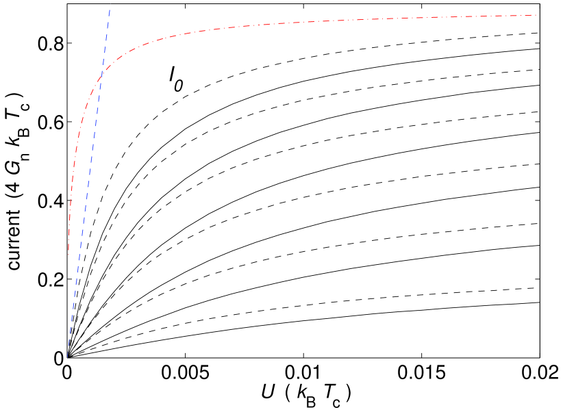
Figure 2: The dc currents $I_{0}$ for temperatures $T/T_{\mathrm{c}}=0.4,0.5,0.6,0.7,0.8,0.9$ in order of decreasing amplitude. The solid lines include the gap suppression effects, whereas in the dashed lines it is neglected. The dash-dotted line is the zero-temperature result of Eq. (34), while the straight dashed line corresponds to Eq. (33) at $T/T_{\mathrm{c}}=0.4$. The results are similar for both parallel and antiparallel $\hat{{\bf{n}}}^{{\rm{l}},{\rm{r}}}$’s. Here $F_{1}^{a}=0$ and $a=1.6$.

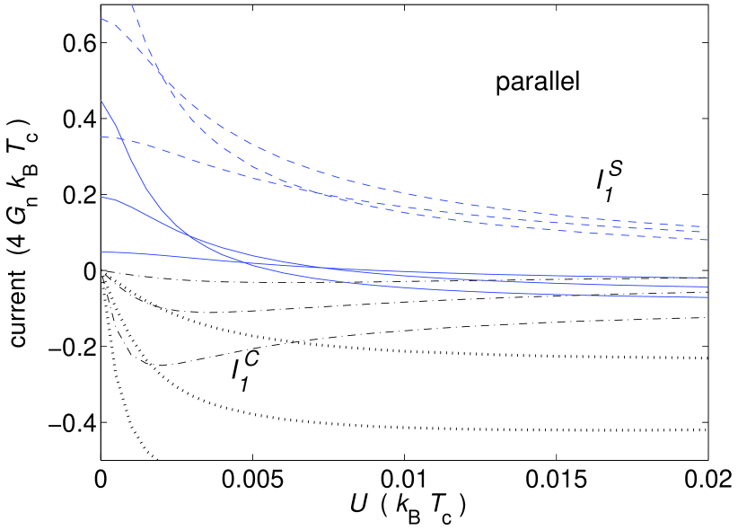
Figure 3: The amplitudes $I^{\mathrm{S}}_{1}$ and $I^{\mathrm{C}}_{1}$ for $T/T_{\mathrm{c}}=0.4,0.6,0.8$ in order of decreasing amplitude in the case of parallel $\hat{{\bf{n}}}^{{\rm{l}},{\rm{r}}}$’s. The solid and dashed lines are for $I^{\mathrm{S}}_{1}$ with and without gap suppression, respectively, and the dash-dotted and dotted lines are the corresponding values for $I^{\mathrm{C}}_{1}$. Here $F_{1}^{a}=0$ and $a=1.6$.

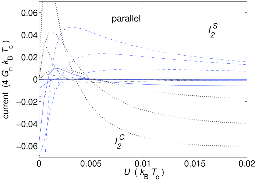
Figure 4: Same as Fig. 3 but for $I^{\mathrm{S}}_{2}$ and $I^{\mathrm{C}}_{2}$.

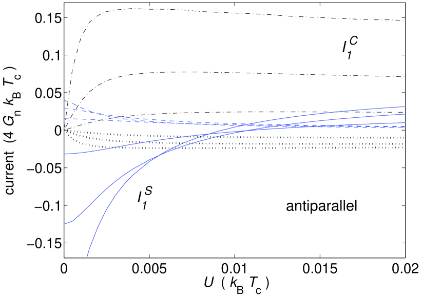
Figure 5: Same as Fig. 3 but for antiparallel $\hat{{\bf{n}}}^{{\rm{l}},{\rm{r}}}$’s

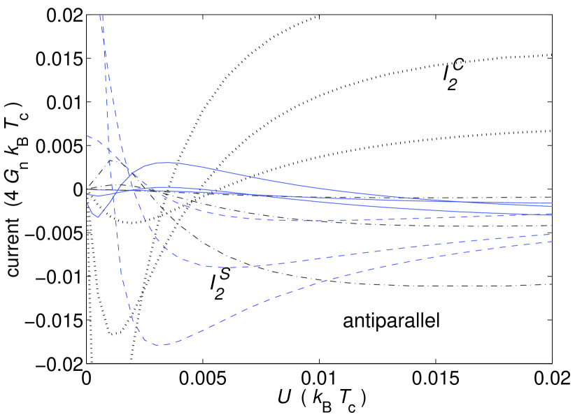
Figure 6: Same as Fig. 4 but for $I^{\mathrm{S}}_{2}$ and $I^{\mathrm{C}}_{2}$.

V.2 Current amplitudes

Figures 2-6 show our results for the lowest-order current amplitudes $I_{0}$, $I^{\mathrm{S}}_{1,2}$ and $I^{\mathrm{C}}_{1,2}$ as a function of the bias $U$. The amplitudes $I^{\mathrm{S}}_{m}$ and $I^{\mathrm{C}}_{m}$ for $m\geq 3$ may be set to zero since they are negligibly small for all practical purposes. Figures 3 and 4 are for parallel $\hat{{\bf{n}}}$’s on the two sides of the contact ($\hat{{\bf{n}}}^{\rm{l}}=\hat{{\bf{n}}}^{\rm{r}}=\hat{{\bf{z}}}$) and Figs. 5 and 6 are for the antiparallel case ($-\hat{{\bf{n}}}^{\rm{l}}=\hat{{\bf{n}}}^{\rm{r}}=\hat{{\bf{z}}}$). The $I_{0}$ amplitude shown in Fig. 2 is the same for both cases. Actually, as our numerical calculation shows, the result for $I_{0}$ is practically independent $R^{{\rm{l}},{\rm{r}}}$. For the case where gap suppression is neglected, this independence was previously shown to be exact — see Eqs. (22) and (25).

In the calculations, we have always assumed $F_{l}^{a}=0$ for $l\geq 3$, while the effect of the remaining $F_{1}^{a}$ with values between $-1\ldots 0$ on the pinhole currents is at most a few percent of their total amplitude Viljas2 — in the figures of this paper $F_{1}^{a}=0$ also. The quasiparticle relaxation parameter is chosen as $a=1.6$, since this is the value which gives the best fit to the relevant experiments — see Sec. VI. Although the behavior of the current amplitudes for $U\lesssim\hbar\Gamma$ depends strongly on the choice of $a$, the asymptotic behavior for $U\gg\hbar\Gamma$ does not.

We have only calculated the currents numerically down to $T/T_{\mathrm{c}}=0.4$, although Fig. 2 shows the additional zero-temperature result of Eq. (34). This is because the required number of terms in the MAR sum [Eq. (16)] is proportional to $\Delta/\Gamma_{0}$, which is on the order of thousands already at $T/T_{\mathrm{c}}=0.4$. We have taken into account all terms up to $n=4\Delta/\hbar\Gamma_{0}$. Actually, this is only necessary for $U\ll\hbar\Gamma$ where the number of successive Andreev reflections is limited by relaxation. In this regime it would also be possible to use approximate schemes instead of the full expression (16). On the other hand, for $U\gtrsim\hbar\Gamma$ a maximum of $\sim\Delta/U$ terms should be enough. The energy cutoff for the coherence functions was typically chosen at around $10k_{\mathrm{B}}T_{\mathrm{c}}$, and the density of energy discretization points was highest close to the gap edges, where the highest accuracy is needed. For energies in between these points, linear interpolation was used in computing the current amplitudes with Eq. (16). The number of Gaussian polar angles used in angular integrals was usually eight.

In the limit $U\rightarrow 0$ the cosine amplitudes $I^{\mathrm{C}}_{m}$ all vanish (linearly in $U/\hbar\Gamma_{0}$) as they should, since the equilibrium current $I_{\rm s}(\phi)$ must satisfy the time-reversal symmetry $I_{\rm s}(-\phi)=-I_{\rm s}(\phi)$. Upon inserting the $I^{\mathrm{S}}_{m}$ amplitudes to Eq. (17) in this limit, the current-phase relations $I_{\rm s}(\phi)$ of Ref. Viljas2, are quite accurately reproduced, when we make the replacement $\omega_{J}t\rightarrow\phi$. Note, in particular, that in the antiparallel case with no gap suppression, the second-order amplitudes are of equal magnitude with the first-order ones. Thus $I_{\rm s}(\phi)$ exhibits a strong “$\pi$ state” Yip . When the gap-suppression effect is taken into account, the $m=2$ amplitudes tend to be very strongly suppressed, and in this case the “$\pi$ state” only presents itself at very low temperatures Viljas2 . Thus as a first approximation, $I^{\mathrm{S}}_{2}$ may often be neglected in comparison with $I^{\mathrm{S}}_{1}$. However, apart from the limit $U\ll\hbar\Gamma$ of very low biases, the cosine amplitude $I^{\mathrm{C}}_{1}$ as well as the dc component $I_{0}$ are equally large as the sine amplitude $I^{\mathrm{S}}_{1}$. Therefore the models which are based on $I^{\mathrm{S}}_{1}$ alone — like that of Ref. Viljas2, — are only valid for $U\ll\hbar\Gamma$ and $T$ close to $T_{\mathrm{c}}$.

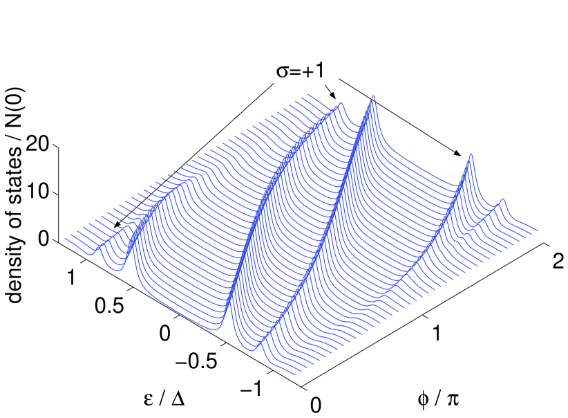
Figure 7: Local density of states inside the pinhole for $\hat{k}_{z}=0.93$ and $-\hat{{\bf{n}}}^{l}=\hat{{\bf{n}}}^{r}=\hat{{\bf{z}}}$ when gap suppression at a diffusive wall is included. Here a large, arbitrary value $a\approx 75$ was chosen for purposes of illustration, in order to make the width $\sim\hbar\Gamma$ of the bound-state peaks better observable. Among the peaks, those corresponding to the $\sigma=+1$ ($\sigma=-1$) spin branch are the ones apparently shifted toward smaller (larger) $\phi$. Note that the slope of the bound states is not so steep as for Eq. (26). Also, for given phase difference and spin band, more than one bound state can exist simultaneously.

V.3 Bound states

In Sec.  IV we saw that in the adiabatic regime $U\ll\Delta$, the currents in the point contact may simply be described in terms of the equilibrium bound states. It should be possible to generalize this description to the case where gap-suppression is included. To study this, we have calculated numerically the density of quasiparticle states at the pinhole. The bound states are given by the sub-gap peaks in the ${\hat{{\bf{k}}}}$-resolved local density of states (or spectral density)

$$N({\hat{{\bf{k}}}},{\bf{R}};\epsilon)=-\frac{N(0)}{\pi}\mathop{\rm{Im}}{\mathop{\mathrm{Tr}}}g^{R}({\hat{{\bf{k}}}},{\bf{R}};\epsilon).$$ (41)

These peaks correspond to poles of $\hat{g}^{R}$, which depend on the phase difference $\phi=\varphi^{\rm{r}}-\varphi^{\rm{l}}$ and the rotation matrices through $\psi_{ij}=R_{\mu i}^{{\rm{l}}}R_{\mu j}^{{\rm{r}}}$. The width of the peaks is on the order of the relaxation rate $\hbar\Gamma$. Although the spectral weight of the bound states is spread around the pinhole up to distances of order $\hbar v_{\mathrm{F}}/\sqrt{\Delta^{2}-\epsilon^{2}}$, we only calculate Eq. (41) inside the hole, at ${\bf{R}}={\bf{0}}$.

Figure 7 illustrates the results for one choice of $\psi_{ij}$ and ${\hat{{\bf{k}}}}$ with $\phi=0\ldots 2\pi$ when the gap suppression effect of a diffusive surface is included. Since $\psi_{ij}\neq\delta_{ij}$, the bound-state peaks in the densities show clearly a spin-splitting between the “$\sigma=\pm 1$” condensates, as in the simple analytic result (26). Since the splitting angle depends on ${\hat{{\bf{k}}}}$, an average of $N({\hat{{\bf{k}}}},\epsilon)$ over the Fermi surface in fact leads to the a formation of a wide band of bound state energies. The bound states for $-{\hat{{\bf{k}}}}$ are obtained by using the time-reversal symmetry ${\hat{{\bf{k}}}}\rightarrow-{\hat{{\bf{k}}}}$, $\phi\rightarrow-\phi$, $\sigma\rightarrow-\sigma$, and the “particle-hole” symmetry ${\hat{{\bf{k}}}}\rightarrow-{\hat{{\bf{k}}}}$, $\epsilon\rightarrow-\epsilon$, which follows from the symmetries of the equations of motion and the geometry ZhangKurkijarviThuneberg .

Compared to Eq. (26), it is seen that the gap suppression modifies the bound states such that they are always at energies $|\epsilon|<\Delta$. In the bulk $N({\hat{{\bf{k}}}},\epsilon)\approx 2N(0)\theta(|\epsilon|-\Delta)|\epsilon|/\sqrt{\epsilon^{2}-\Delta^{2}}$ has divergences at $|\epsilon|=\Delta$, but in the middle of the junction most of the spectral weight is now in the bound states even at $\phi=0$. Thus there are several branches of bound states coexisting simultaneously for given $\phi$. Accordingly, Eq. (29) for the current should be modified by replacing $\epsilon_{{\hat{{\bf{k}}}},\sigma}(\phi)$ with $\epsilon_{q,{\hat{{\bf{k}}}},\sigma}(\phi)$, and by adding a sum over the branch index $q$. Since the energies $\epsilon_{q,{\hat{{\bf{k}}}},\sigma}(\phi)$ for a given branch in the range $(-\Delta,\Delta)$ are now mapped to phase differences in the range $(-\infty,\infty)$, their slopes are not so steep. Therefore, one would expect that the dc currents are generally smaller when the gap suppression effect is taken into account. As seen in Fig. 2, this is usually the case.

VI Comparison to experiment

In this section we present a brief comparison of the above theory to available experimental data on the current-pressure characteristics in ³He-B weak links Steinhauer ; Simmonds . There are a couple of basic things to note about the experiments. First, as already mentioned, it is difficult to manufacture apertures which would satisfy the requirements of a pinhole very well DavisPackardRMP . The apertures with $d\approx 100$ nm in a 50 nm membrane used in Ref. Simmonds, are rather close, at least compared with the 0.25 $\mu$m wide slits in a 0.1 $\mu$m membrane of Ref. Simmonds . Second, in order to ensure leak-proofness, the pressure biases are limited to very low values where $U\ll\Delta$. The experiments of Ref. Simmonds, are even restricted to $U\ll\hbar\Gamma\ll\Delta$. Therefore, the “excess current” limit of Eq. (35), for example, seems not practically achievable in superfluid ³He. Nevertheless, the data of Refs. Steinhauer, ; Simmonds, are enough to make a comparison between the most important features of the theoretical and experimental current-pressure characteristics.

Figure 8 shows a comparison between the data of Ref. Steinhauer, and the numerical pinhole calculation of $I_{0}(U)$.

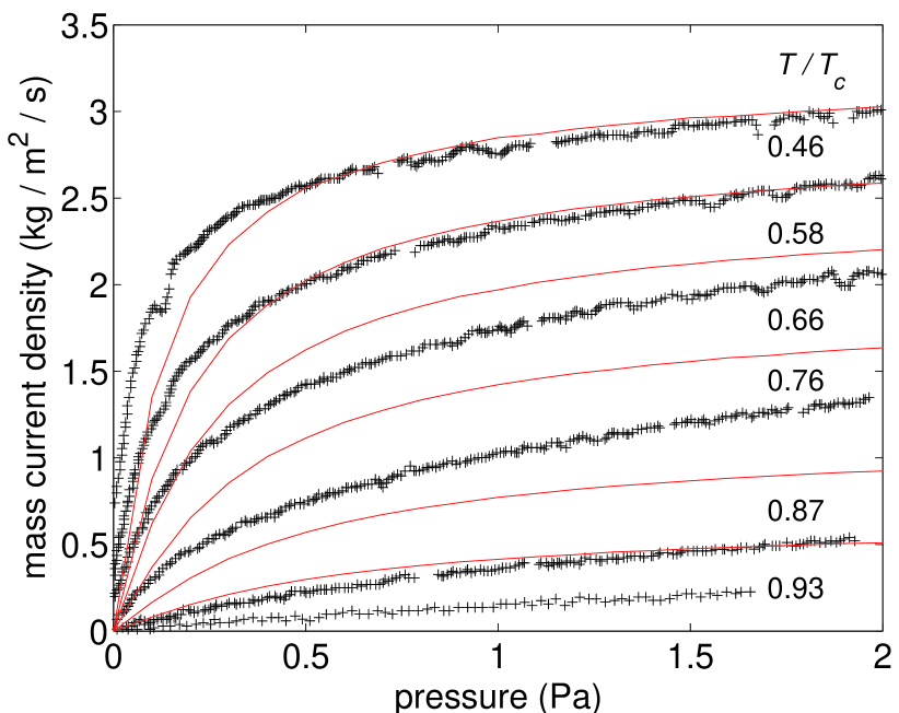
Figure 8: Comparison of the data (+ signs) from Ref. Steinhauer, to the pinhole theory (solid lines) for a diffusive surface and $a\approx 0.27$ at indicated temperatures.

A diffusive surface is assumed, and we use the parameter $a\approx 0.27$. Again we note that although the slope at $U=0$ depends strongly on $a$, the asymptotic behavior for $U\gg\hbar\Gamma$ does not. Indeed, at $U\gtrsim\hbar\Gamma$ the agreement is rather good for any value of $a$ on the order of unity, although a perfect fit for all temperatures simultaneously cannot be achieved. Note also that the experimental currents are not even approaching zero in the limit $U\rightarrow 0$. However, a better fit can hardly be expected, since the apertures used in these experiments were far from good pinholes. In fact, in sufficiently large apertures one would expect a transition into a regime where the dissipation is best described in terms of phase slips by vortices rather than MAR. Studying this transition would be interesting, but computationally very demanding. In any case, the overall form of $I_{0}(U)$ is very similar to the experimental results, and the order-of-magnitude agreement on both axes is surprisingly good. This gives strong support to the expectation that the dominating dissipation mechanism in small apertures of superfluid ³He is the MAR process, analogously to superconductor point contacts.

The apertures used in the experiments reported in Ref. Simmonds, are somewhat better approximations to pinholes. Therefore we have chosen to use these data to estimate the value of $a$ for the numerical calculations of the previous Section. The experiments were carried out in the limit $U\ll\hbar\Gamma$, and according to Eq. (33), the current should be linear in the bias. For the “L state” this is rather well satisfied, and a fit to the L-state data gives $a\approx 1.6$, when gap suppression at a diffusive surface is taken into account Viljas5 . The fit is shown in Fig. 9.

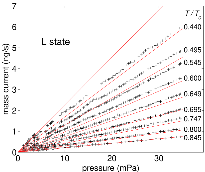
Figure 9: Comparison of the L state data (+ signs) from Ref. Simmonds, to the pinhole theory (solid lines) for a diffusive surface and $a\approx 1.6$ at indicated temperatures.

The increasing low-temperature deviations in this fit may be partly due to the insufficiency of our normal-state model for $\Gamma$. The currents for the “H state” reported in Ref. Simmonds, are larger and more nonlinear than in the L state. We suspect that part of this nonlinearity may be due to the additional dissipation effects described by Eq. (37) Viljas5 . Another possibility is that the experimental apertures already deviate so strongly from pinholes, that the dependence of the bound states on textures is not sufficiently described by simple phase shifts.

VII Conclusions and discussion

In conclusion, we have presented an analysis of pressure-biased weak links between two volumes of superfluid ³He-B by using the pinhole model of a short, ballistic point contact. We showed how the $s$-wave results of Refs. GunsenheimerZaikin, ; AverinBardas, may easily be reproduced and generalized to the $p$-wave case by parametrizing the Green functions with the so-called coherence functions. In the case where the gap suppression at surfaces is neglected, we calculated the current amplitudes analytically in several limits. In the general case, the order parameters and the pinhole currents were calculated numerically. Comparison to experiments gives strong support to the existence of the MAR effect in pressure-biased weak links of superfluid ³He Steinhauer . We also predict the existence of additional dc current contributions, which result from the excitation of collective order-parameter modes. These “anisotextural” effects are discussed elsewhere in more detail Viljas5 .

In order to improve upon the results of the present paper, one should take into account the strong-coupling effects in a more detailed way than with our “normal-state” model for the quasiparticle relaxation rate. One should also consider apertures of finite size, at least by computing the bound-state spectra in equilibrium to see if textures have some significant effect on them in this case. A dynamical calculation for the finite-size aperture should also be performed, but this already seems to approach the limits of practical feasibility. A fully self-consistent calculation of the anisotextural effects in a pressure-biased pinhole array also appears to be very difficult. However, until such improvements are made, a parameter-free comparison with the experimental data cannot be expected.

With somewhat less effort, the pinhole heat conductivity EskaHeat or spin currents could be studied by starting from Eq. (13). The current-noise properties AverinImam of a ³He pinhole could also be of some interest, for example in the design of accurate superfluid ³He gyrometers AvenelMukharsky .

Appendix A Equilibrium equations

Close to the planar wall at $z=0$ the mean-field self energies and the coherence functions must be iterated self-consistently. Since we are concerned with an equilibrium system, it is easiest to do this by using the Matsubara technique, where one makes an analytical continuation from the real energies $\epsilon^{R,A}=\epsilon\pm{\mathrm{i}}0^{+}$ to the imaginary Matsubara energies $\pm{\mathrm{i}}|\epsilon_{m}|$, where $\epsilon_{m}(T)=\pi k_{\mathrm{B}}T(2m+1)$ and $m=0,\pm 1,\pm 2,\ldots$ SereneRainer . The coherence functions are then obtained from Eq. (39), where $\epsilon^{R}\rightarrow{\mathrm{i}}\epsilon_{m}$ and $\gamma_{0}^{R}(\epsilon)\rightarrow\gamma_{0}(\epsilon_{m})$. (Here we take $\Gamma_{1}$ as infinitesimal.) The self-energies are of the form $\Delta_{0}=\boldsymbol{\Delta}_{0}\cdot\boldsymbol{\sigma}{\mathrm{i}}\sigma_{2}$ and $\Sigma^{\rm mf}_{0}=\boldsymbol{\nu}_{0}\cdot\boldsymbol{\sigma}$. If we use the symmetry $\tilde{\boldsymbol{\nu}}_{0}=-\boldsymbol{\nu}_{0}$ SereneRainer ; Viljas2 , the solution of Eq. (39) may be parametrized by $\gamma_{0}=\boldsymbol{\gamma}_{0}\cdot\boldsymbol{\sigma}{\mathrm{i}}\sigma_{y}$, and the equation becomes

$$\begin{split}{\mathrm{i}}\hbar{\bf{v}}_{\mathrm{F}}\cdot\boldsymbol{\nabla}\boldsymbol{\gamma}_{0}=&-2{\mathrm{i}}\epsilon_{m}\boldsymbol{\gamma}_{0}-\boldsymbol{\Delta}_{0}-2(\boldsymbol{\gamma}_{0}\cdot\boldsymbol{\Delta}_{0}^{*})\boldsymbol{\gamma}_{0}\\ &+(\boldsymbol{\gamma}_{0}\cdot\boldsymbol{\gamma}_{0})\boldsymbol{\Delta}_{0}^{*}+2{\mathrm{i}}\boldsymbol{\nu}_{0}\times\boldsymbol{\gamma}_{0}.\end{split}$$ (42)

Due to translational symmetry along the wall, the solution and the self-energies only depend on the coordinate $z$. The self-consistency equations are given by SereneRainer

$$\begin{split}\boldsymbol{\Delta}_{0}({\hat{{\bf{k}}}},z)&=3k_{\mathrm{B}}TV_{1}\sum_{|\epsilon_{m}|<\epsilon_{c}}\left\langle({\hat{{\bf{k}}}}\cdot{\hat{{\bf{k}}}}^{\prime}){\bf{f}}_{0}({\hat{{\bf{k}}}}^{\prime},z,\epsilon_{m})\right\rangle_{{\hat{{\bf{k}}}}^{\prime}}\\ \end{split}$$ (43)

where the $p$-wave pairing interaction $V({\hat{{\bf{k}}}}\cdot{\hat{{\bf{k}}}})=3V_{1}{\hat{{\bf{k}}}}\cdot{\hat{{\bf{k}}}}^{\prime}$ was assumed, and

$$\begin{split}\boldsymbol{\nu}_{0}({\hat{{\bf{k}}}},z)&=3k_{\mathrm{B}}T\sum_{|\epsilon_{m}|<\epsilon_{c}}\left\langle A_{a}({\hat{{\bf{k}}}}\cdot{\hat{{\bf{k}}}}^{\prime}){\bf{g}}_{0}({\hat{{\bf{k}}}}^{\prime},z,\epsilon_{m})\right\rangle_{{\hat{{\bf{k}}}}^{\prime}}.\end{split}$$ (44)

In these $\langle\cdots\rangle_{{\hat{{\bf{k}}}}}=\int({\mathrm{d}}\Omega_{\hat{{\bf{k}}}}/4\pi)(\cdots)$, ${\bf{g}}_{0}={\mathop{\mathrm{Tr}}}_{2}(\boldsymbol{\sigma}g_{0})/2$, ${\bf{f}}_{0}=-{\mathop{\mathrm{Tr}}}_{2}(\boldsymbol{\sigma}g_{0}{\mathrm{i}}\sigma_{2})/2$ where the upper diagonal and off-diagonal Nambu components of the Matsubara propagator $\hat{g}({\hat{{\bf{k}}}},z,\epsilon_{m})$ are given by $g_{0}=-\pi{\mathrm{i}}(1+\gamma_{0}{\tilde{\gamma}}_{0})(1-\gamma_{0}{\tilde{\gamma}}_{0})^{-1}$ and $f_{0}=-2\pi{\mathrm{i}}\gamma_{0}(1-\gamma_{0}{\tilde{\gamma}}_{0})^{-1}$. The conjugation symbol “$~{}\tilde{~}{}~{}$” now means ${\tilde{\gamma}}_{0}({\hat{{\bf{k}}}},\epsilon_{m})=\gamma_{0}(-{\hat{{\bf{k}}}},\epsilon_{m})^{*}$ $=[\gamma_{0}({\hat{{\bf{k}}}},-\epsilon_{m})]^{\dagger}$. The coupling constant $V_{1}$ may be eliminated in the usual way by noting that at $T\rightarrow T_{\mathrm{c}}^{-}$ the gap vector $\boldsymbol{\Delta}_{0}$ is small and ${\bf{f}}_{0}\approx\pi\boldsymbol{\Delta}_{0}/|\epsilon_{m}|$. Thus $\boldsymbol{\Delta}_{0}$ may be canceled and one finds

$$\begin{split}V_{1}^{-1}&\approx\pi k_{\mathrm{B}}T_{c}\sum_{|\epsilon_{m}|<\epsilon_{c}}|\epsilon_{m}|^{-1}+\ln(T/T_{\mathrm{c}})\end{split}$$ (45)

where $\epsilon_{m}=\epsilon_{m}(T)$. Inserting this into Eq. (43), the cutoff $\epsilon_{c}$ may be taken to infinity — see Eq. (12) in Ref. Viljas2, . The function $A_{a}(x)=\sum_{l=0}^{\infty}F_{l}^{a}[1+F_{l}^{a}/(2l+1)]^{-1}P_{l}(x)$, where $P_{l}(x)$ are the Legendre polynomials. From symmetries of the planar wall geometry it follows that if ${\hat{{\bf{k}}}}$ is in the $xz$ plane, so are ${\bf{f}}_{0}$, $\boldsymbol{\Delta}_{0}({\hat{{\bf{k}}}})=\Delta_{\parallel}\hat{k}_{x}\hat{{\bf{x}}}+\Delta_{\perp}\hat{k}_{z}\hat{{\bf{z}}}$ and $\boldsymbol{\gamma}_{0}$, while ${\bf{g}}_{0}$ and $\boldsymbol{\nu}_{0}({\hat{{\bf{k}}}})=\nu_{0y}({\hat{{\bf{k}}}})\hat{{\bf{z}}}$ are perpendicular to it. Also due to symmetries, all $F_{l}^{a}$ with even $l$ drop out of the theory, and for $l\geq 3$ we assume them to be zero Viljas2 .

In the bulk $\boldsymbol{\Delta}_{0}$ is constant and $\boldsymbol{\nu}_{0}=0$, so that Eq. (42) is easily solved, and this solution is used as an initial condition on trajectories starting from the bulk. On the wall side, one needs a boundary condition to compute the “outgoing” coherence functions from the “incoming” functions. We use the ROM boundary condition, which is explained in Ref. ROM, . This is easiest to express in terms of the components of the propagator $\hat{g}({\hat{{\bf{k}}}},z,\epsilon_{m})$, rather than directly with the coherence functions $\gamma_{0}({\hat{{\bf{k}}}},z,\epsilon_{m})$. The relation $\gamma_{0}=-({\mathrm{i}}\pi-g_{0})^{-1}f_{0}$ is then useful for computing the initial condition for $\gamma_{0}$ on the outgoing trajectories VorontsovSauls . A specularly reflecting surface is much simpler to implement, since it only leads to the the continuity condition $\gamma_{0}(\underline{{\hat{{\bf{k}}}}})=\gamma_{0}({\hat{{\bf{k}}}})$, where $\underline{{\hat{{\bf{k}}}}}={\hat{{\bf{k}}}}-2({\hat{{\bf{k}}}}\cdot\hat{{\bf{z}}})\hat{{\bf{z}}}$ is the specularly reflected direction. As shown in Ref. Viljas2, , the pinhole current amplitudes for specular and diffusive surfaces usually have only minor (at most a few percent) differences. Thus, in practice the implementation of a diffusive surface may not be worth the trouble.

Appendix B Folding products

The quasiclassical folding product between objects of the type $\hat{A}(\epsilon,t)$ is defined in Ref. SereneRainer, . This result is generalized to multiple products of $n$ objects $\hat{A}_{j}(\epsilon,t)$, $j=1,2,\ldots,n$ as follows

$$\begin{split}(\hat{A}_{1}&\circ\cdots\circ\hat{A}_{n})(\epsilon,t)\\ &=\prod_{j=1}^{n}\hat{A}_{j}[\epsilon+\frac{\hbar}{2{\mathrm{i}}}(\cdots+\partial_{j-1}-\partial_{j+1}-\cdots),t_{j}],\end{split}$$ (46)

assuming all the Fourier-transformations leading to the “mixed” representations $\hat{A}_{j}(\epsilon,t)$ exist. Here $\partial_{j}$ refers to a derivative with respect to the $j$th time variable $t_{j}$. When the time dependence of $\hat{A}_{j}(\epsilon,t)$ is harmonic [i.e., $\propto\exp({\mathrm{i}}\epsilon t/\hbar)$], Eq. (46) yields the folding product analytically. In equilibrium all time derivatives vanish, and the folding product becomes a simple matrix product.

References

• (1) D. Vollhardt and P. WΓΆlfle, The superfluid phases of helium three (Taylor & Francis, London, 1990).
• (2) J. KurkijΓ€rvi and D. Rainer, in Helium Three, eds. W. P. Halperin and L. P. Pitaevskii, pp. 313-351 (Elsevier, Amsterdam, 1990)
• (3) J.C. Davis and R.E. Packard, Rev. Mod. Phys. 74, 741 (2002).
• (4) I. O. Kulik and A. N. Omel’yanchuk, Fiz. Nizk. Temp. 4, 296 (1978) [Sov. J. Low Temp. Phys. 4, 142-149 (1978)]
• (5) A. V. Zaitsev, Zh. Eksp. Teor. Fiz. 78, 221 (1980); [Sov. Phys. JETP 51, 111 (1980)].
• (6) D. Averin and A. Bardas, Phys. Rev. B 53, R1705 (1996).
• (7) D. Averin and H. T. Imam, Phys. Rev. Lett. 76, 3814 (1996).
• (8) U. Gunsenheimer and A. D. Zaikin, Phys. Rev. B 50, 6317 (1994).
• (9) M. Octavio, et al., Phys. Rev. B 27, 6739 (1983).
• (10) J. K. Viljas and E. V. Thuneberg, J. Low Temp. Phys. 134, 743 (2004).
• (11) J. K. Viljas and E. V. Thuneberg, Phys. Rev. B 65, 064530 (2002).
• (12) J. Steinhauer, et al., Physica B 194-196, 767 (1994).
• (13) R. W. Simmonds, et al., Phys. Rev. Lett. 84, 6062 (2000)
• (14) C. J. Bolech and T. Giamarchi, Phys. Rev. Lett. 92, 127001 (2004).
• (15) N. B. Kopnin, Phys. Rev. B 65, 132503 (2002).
• (16) J. K. Viljas and E. V. Thuneberg, cond-mat/0401637.
• (17) J. W. Serene and D. Rainer, Phys. Rep. 101, 221 (1983).
• (18) N. Schopohl and K. Maki, Phys. Rev. B 52, 490 (1995).
• (19) Y. Nagato, K. Nagai, and J. Hara, J. Low Temp. Phys 93, 33 (1993).
• (20) M. Eschrig, Phys. Rev. B 61, 9061 (2000).
• (21) V. Ambegaokar, P. G. deGennes, D. Rainer, Phys. Rev. A 9, 2676 (1974).
• (22) S.-K. Yip, Phys. Rev. Lett. 83, 3864-3867 (1999).
• (23) A. Barone and G. Paterno, Physics and Applications of the Josephson Effect, (John Wiley & Sons, New York, 1982).
• (24) L. J. Buchholtz, and D. Rainer, Z. Phys. 35, 151 (1979).
• (25) W. Zhang, J. KurkijΓ€rvi, and E. V. Thuneberg, Phys. Rev. B 36, 1987 (1987).
• (26) N. B. Kopnin, P. I. Soininen, and M. M. Salomaa, J. Low Temp. Phys. 85, 267 (1991).
• (27) E. V. Thuneberg, M. FogelstrΓΆm, and J. KurkijΓ€rvi, Physica B 178, 176 (1992).
• (28) J. C. Wheatley, Rev. Mod. Phys. 47, 415 (1975).
• (29) D. S. Greywall, Phys. Rev. B 33, 7520 (1986).
• (30) S. V. Pereverzev and G. Eska, proceedings of the symposium on Quantum Fluids and Solids 2004, J. Low Temp. Phys., to be published.
• (31) O. Avenel, Yu. Mukharsky, and E. Varoquaux, J. Low Temp. Phys. 135, 745 (2004).
• (32) A. B. Vorontsov and J. A. Sauls, Phys. Rev. B 68, 064508 (2003).