Anti-deterministic behavior of discrete systems
that are less predictable than noise

Abstract

We present a new type of deterministic dynamical behaviour that is less predictable than white noise. We call it anti-deterministic (AD) because time series corresponding to the dynamics of such systems do not generate deterministic lines in Recurrence Plots for small thresholds. We show that although the dynamics is chaotic in the sense of exponential divergence of nearby initial conditions and although some properties of AD data are similar to white noise, the AD dynamics is in fact less predictable than noise and hence is different from pseudo-random number generators.

I Introduction

Determinism in the strict sense is defined by the existence of a unique solution of the initial value problem: Given an equation of motion, then the motion generated by it is said to be deterministic if the solution evolving from a given initial condition depends exclusively on the latter, i.e., it is uniquely determined (for all future times) by fixing the initial conditionSchuster . This property is usually contrasted by stochastic motion, where random noises enter the equation of motion, such that the initial condition alone is insufficient to fix the future evolution. One additionally needs to know the realization of the sequence of noise inputs. Without this, one can only make probabilistic statements about the evolving solutions.

In the above restricted sense, the dynamics which we introduce here is in fact deterministic. However, when speaking about determinism, one often considers the aspect of recurrence: Determinism implies that when, in the course of time, the system returns to a state which it has assumed before, the evolution will repeat itself precisely. If in addition (as it is most often the case) the terms in the equation of motion depend smoothly on the state vector, then the return to a similar state will cause a similar future evolution, at least on short times (in chaotic systems, this time is related to the inverse of the Kolmogorov-Sinai entropy). This follows from a simple linearization of the equations around a given reference state and is the basis of many time series tools in reconstructed phase spacesKantzSchreiber . In particular, this is the basis of the famous “Lorenz method of analogues”Lorenz or, more technically speaking, the zeroth order prediction schemeFarmerSidorowich : If one wants to predict the short time future of a deterministic system, the simplest method is to look for situations in the past which are very similar to the present one, and to assume that (because of the above discussed properties of determinism) the future will be similar to what followed the similar situation in the past. In many applications to experimental data, such prediction schemes have in fact been proven to work very successfullyAbarbanel ; KantzSchreiber . What we call anti-deterministic is exactly the opposite: whenever our system comes to a state which is similar to some state of the past, it will evolve in the most different way from the past, so that past information is systematically misleading when trying to make predictions.

This property would require a highly non-smooth equation of motion. Instead, we will define the dynamics not through an equation of motion but by a minimization problem. This is, however, not too unusual, since one can convert every differential equation initial value problem into a variational problem, where the solution on a finite time interval is given by a path which generates the extremum of some functional (compare the principle of minimal action in classical mechanicsGoldstein ).

A particular tool for the visual inspection of this aspect of determinism is the recurrence plotEckmann . A recurrence plot of a given time series $\left\{x_{i}\right\},\;\;i=1,\ldots,N$ is the $N\times N$-matrix ${\bf R}$ with the entries $R_{ij}=\Theta(\varepsilon-|x_{i}-x_{j}|)$, where $\Theta$ is the Heaviside step function. I.e., a matrix element is unity if the correponding time series points are closer than $\varepsilon$, and it is zero else. Such a matrix can be easily represented graphically which is called the recurrence plot, with the parameter $\varepsilon$. Several concepts for a quantitative evaluation of recurrence plots have been proposedZbilut ; Casdagli ; Potsdam .

Based on the theorem of TakensTakens , determinism in the more general sense expresses itself in time series data by the existence of line segments parallel to the diagonal in this plot. The lengths of these lines for periodic or quasiperiodic systems are limited only by the lengths $N$ of the corresponding time series because there is no divergence of nearby trajectories. The lines are much shorter for chaotic motion because of a finite exponential divergence, corresponding to the positive entropy of chaotic systemsCasdagli . The lines themselves are representative of unstable periodic orbits of the system. Also for data stemming from uncorrelated stochastic processes (such as white noise) there exists some small but nonzero probability that a “deterministic” line can occur in a RP for a finite threshold value $\varepsilon$, since similar data segments may occur by chance. The systems which we call anti-deterministic (AD) are designed to create systematically less lines parallel to the diagonal in recurrence plots than white noise, and for certain recurrence parameters they do not possess any line at all.

More specifically, we generate sequences of AD data by requiring them not to create any line of length longer then $n$ in RP maximizing the threshold $\varepsilon$. We found several algorithms that can produce such data in a deterministic way, and presumably one can also introduce some randomness beyond the choice of random initial conditions. In the next section we show one simple procedure. The AD motion does not belong to a class of chaotic systems with a very high entropy (pseudo-random number generatorsNumRec ). As it will become clear in the next section, our construction of AD data requires an infinite memory of the dynamical system, which corresponds to an infinite dimensional phase space. There are neither (unstable) periodic orbits nor is there any attractor. Data corresponding to AD systems cover uniformly the whole admissible phase space.

II A simple algorithm for AD data generation

Working in discrete time, we generate the AD data iteratively. We restrict the individual time series elements $x_{i}$ to be from the unit interval, $x_{i}\in[0,1]\;\;\forall i$. Let $\left\{x_{i}\right\}$ for $i=1,2,\ldots,N$ be a given sequence representing the data up to time $N$. The next time series element $x_{N+1}$ is the one that maximizes its (suitably defined) distance to all previous points of the time series. More precisely, $x_{N+1}$ maximizes the following utility function $U_{x}$:

$$U_{x}=\min\limits_{i=d+m,d+m+1,\ldots,N}\prod_{\kappa=0}^{m}dis_{d}\left(i-\kappa,N+1-\kappa\right)\;.$$ (1)

Here, $m$ and $d$ are parameters of the algorithm, while $dis_{d}\left(i,N+1\right)$ is the Euclidean distance between points $x_{i}$ and $x_{N+1}$ in a $d$-dimensional time delay embedding space:

$$dis_{d}(i,N+1)=\sqrt{\sum\limits_{k=0}^{d-1}\left\|x_{i-k}-x_{N+1-k}\right\|^{2}}\;.$$ (2)

It can be useful to impose periodic boundary conditions on the unit interval when computing the distance, i.e., $\left\|x_{i}-x_{j}\right\|:=min(\left|x_{i}-x_{j}\right|,1-\left|x_{i}-x_{j}\right|)$.

For the simple choice $m=0$, Eq.(1) gives the distance (in the $d$-dimensional time delay embedding space) between the “new” time series point and its closest neighbour among all past points, which, by the choice of the new point, should be as large as possible. For $m>0$, the antideterministic features which we study below become more pronounced. In order to start the algorithm, an initial sequence $\left\{x_{i}\right\}$ for $i=1,2,\ldots,n_{0}$ has to be chosen.

Our algorithm of AD data generation is very simple and one can imagine that this method can be modified in many different ways, e.g., by modifying the function $U_{x}$. As long as the main idea, namely that the new data point (in a time delay embedding sense of TakensTakens ) is required to be far from all previous points, is respected by $U_{x}$, the properties of the resulting data are all very similar. In Fig. (1) an example of an AD time series is shown.

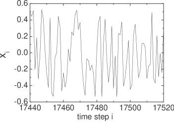
Figure 1: The example of AD time series.

III Properties

The requirement of anti-determinism translates into the fact that there cannot be contracting and not even marginally stable directionsEckmannRuelle in the dynamical system. This type of behavior easily occurs in discrete time where all directions can be divergent. In a conventional flow (continuous time system) there is always one direction corresponding to a zero Lyapunov exponent. Hence, if the generalization of AD to continuous time dynamics is possible it will lead to a nowhere continuous signal similar to white noise. Here, we restrict ourselves to the time discrete version. An AD trajectory never forgets its initial condition $\left\{x_{i}\right\}$, $i=1,2,\ldots,n_{0}$ and it is very sensitive to their changes. As we can see from Fig.2, the divergence of initially nearby solutions is, on average, exponential, resembling low-dimensional chaos. This result is consistent with our statement that AD data are usually no high-entropic data such as those generated by linear congruential random number generators. The specific realization also depends sensitively on the parameters $m$ and $d$. The main feature of AD data is the absence of RP lines of lengths larger than $d$ for small values of $\varepsilon$. In a conventional chaotic sequence, despite the unpredictability in the long run, on short times similar states evolve similarly. This is related to the existence of unstable periodic orbits which are densely embedded in the invariant set for relevant classes of chaotic attractorsOtt . A close approach of the trajectory to an unstable periodic orbit can create a long line in the recurrence plot. Our algorithm sytematically eliminates the possibility of unstable periodic orbits, as one can easily see: A periodic time series, of whatever large period length $T$, would result in $U(x_{N+1})=0$ in Eq.(1) as soon as $N+1\geq T$, hence, the periodic continuation is forbidden by our algorithm.

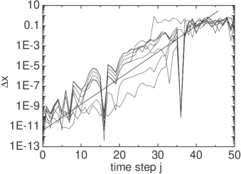
Figure 2: The distance of time series elements $\Delta x=\left\|x_{j}-x^{\prime}_{j}\right\|$ evolving from nearby initial conditions ($n_{0}=50$, $m=4$, $d=2$, perturbation of the initial condition in the range of $10^{-10}$). The line guides the eye and corresponds to the behavior $e^{0.61j}$.

An AD system tries not only not to repeat the past trajectory but to escape from it to other points of the phase space. It follows that although for chaotic systems the attractor dimension is finite and fixed for the AD motion the dimension of an observed trajectory increases with the number of generated points. In this sense the AD systems are infinite dimensional and Unstable Periodic Orbits cannot exist. Neigbouring trajectories in AD systems diverge in all directions and as result there is no system attractor, i.e., the data are confined to a finite volume in space only through the constraints (here: $x_{i}\in[-0.5:0.5]$).

IV Time Series Analysis

The AD data share many properties of white noise, but there are some which do not appear in any another dynamical behaviour. Let us first focus on features common with noisy data. It is easy to check that our AD data converge to the uniform density in the unit interval. The autocorrelation function, the mutual information parameter as well as the power spectrum are for the AD data of Eq.(1) the same as for the white noise, i.e., AD data appear to be uncorrelated.

Of course, by construction, there are subtle long range correlations which have to show up in a suitable analysis. The block correlation entropies $K_{2}^{n}$ offer one such analysis. In terms of RP a line of length $1$ in an embedding dimension $n$ and a line of length $n$ in an embedding dimension $1$ are equivalent Faure . For this reason one can alternatively use terms embedding dimension and length of a line (the embedding dimension used in RP is one for all the calculations). Let us define the number of lines in RP of length $n$ or longer as $DET_{n}(\varepsilon)$ urb03 . Then the coarse-grained block correlation entropy can be defined as Proccacia

$$K_{2}^{n}(\varepsilon)=\ln\frac{DET_{n}(\varepsilon)}{DET_{n+1}(\varepsilon)}$$ (3)

and it corresponds to the slope in the plot $\ln DET_{n}$ versus $n$. The differences between the noise and AD data can be seen very clearly when we plot the coarse-grained block correlation entropy $K_{2}^{n}$ versus the embedding dimension $n$ (see Fig. 3). The entropy of AD data measured from numbers $DET_{n}(\varepsilon)$ of lines of length $n=3$ or longer is higher than the white noise entropy which in Fig. 3 is a straight line with the slope $-\ln(10)$. The minimal threshold for which the entropy can be calculated for $n=3$ corresponds to the maximal $\varepsilon_{max}$ for which there are no lines in RP of the length $n=3$ or longer. The maximal entropies which can be obtained from a finite time series of white noise and of the AD time series of the same length are the same, but the maximum for AD data is always reached with larger values of $\varepsilon_{max}$ as compared to noisy data.

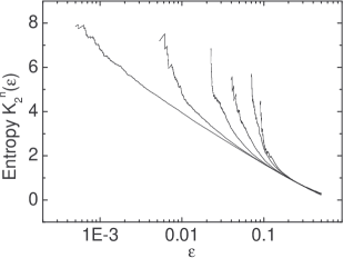
Figure 3: Coarse-grained block correlation entropy calculated for AD systems with $d=2$, $m=4$. Curves from the left to right correspond to embedding dimensions increasing from $n=2$ to $n=7$ while the straight line corresponds to entropy of white noise. The inset shows schematically the behaviour of the coarse-grained correlation entropy for different types of motion: (dashed dotted line) deterministic systems (D), (dashed line) white noise (WN) and (solid line) AD.

The same feature of AD data can be analyzed from another point of view. We have calculated the minimal distance between nearest neighbors for the whole data set and have divided it by the same quantity of shuffled data. Because for random data the minimal distance between nearest neighbors can differ for different shuffling an appropriate averaging has been performed. In such a way we create a parameter that we call $ADET_{n}$ which is a measure how much data are anti-deterministic ($n$ is here an embedding dimension). We have checked that for chaotic data with noise and for large $n$ this parameter converges to the noise level

$$NTS=\frac{\sigma_{noise}}{\sigma_{DATA}}\;,$$ (4)

where $\sigma_{noise}$ is the standard deviation of noise and $\sigma_{DATA}$ stands for the standard deviation of data. Hence, for (noisy) deterministic data it is usually much smaller than unity. Shuffling makes no difference for random data and hence $ADET_{n}=1$. Fig. 4 shows a plot of values $ADET_{n}$ versus $n$ for AD data with $d=2$ and $m=4$. One can see that for $n$ between $4$ and $7$ we have $ADET_{n}\approx 1.75$ what means that the mean minimal distance between nearest neighbors for AD data is about $1.7$ times larger than for noisy data, and very much larger than for conventional deterministic data.

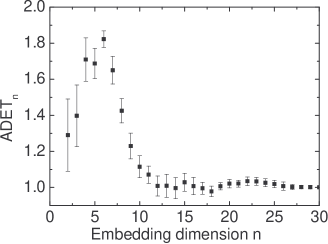
Figure 4: The plot of parameter $ADET_{n}$ versus $n$ ($d=2$ and $m=4$).

To demonstrate that AD data are less predictable than noise we have calculated a prediction error that one receives from a zeroth order predictionFarmerSidorowich using the nearest neighbor. This simple forecasting method shows clearly that our AD data are less predictable than noise, i.e., than randomly shuffled data (see Fig. 5). The average prediction error for noisy data should equal $\sqrt{2}$ because we have the root mean square of a quantity which is the sum of two random numbers, and the error of our AD data is larger for a range of embedding dimensions.

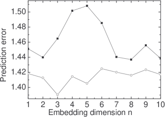
Figure 5: The prediction error divided by standard deviation of data for AD data ($d=2$, $m=4$) and for randomly shuffled data.

Long range correlations in data may also express themselves in anomalous diffusion properties when integrating the dataDFA . This can be quantified by the Hurst exponent. The Hurst exponent of data generated by Eq.(1) is found to be 1/2, which is the value of white noise. However, using a different, more complicated algorithm (see appendix A), we were able to create data which are anti-persistent, i.e., for which we found Hurst exponents ranging from $0.15$ to $0.5$, depending on parameters in the algorithm. Observing histograms of such data we have found that for finite time series lengths, the data can be much more uniformly distributed than for standard noise generators (used commonly in C compilers). Thanks to this property one can generate very short time series with a very flat histogram.

V Applications

There may be different useful applications of AD data. One of them are noise generators. Common features of AD data and noisy data are in this case very desired. Some of the properties can be modified changing the method and its parameters, e.g., to get a desired anti-persistence. The big advantage here might be given by the property that histograms converge much faster to their limiting shape than for uncorrelated random numbers, so that smaller samples might yield sample means which are closer to the true mean than for truly random samples. In Monte Carlo methods for searching global minima, the feature of having large minimal distances might enhance the efficiency due to the fact that it is less likely to converge to the same local minimum with another initial condition from the sample.

The AD systems can also be used in data encryption because noisy behavior makes unwanted deciphering very difficult. As we mentioned, there are many ways of how to modify the method generating AD data which can produce entirely different time series. One can imagine that an encryption key can be parameters of a modificated scheme.

We suspect that AD behaviour can be observed in nature as well. One evident possibility is to see it as results of games when an intelligent player tries to find a strategy that would be as much as possible unpredictable to an intelligent opponent. This can occur in predator-prey relations as well as in economical processes. In physics, adding one by one charged particles to a set of fixed charges with the requirement of consuming minimal energy would result in a sequence of positions of the added particles which is generated by a functional similar to Eq.(1), $U_{x}=\left(\sum_{i=1}^{N}\frac{1}{\left|x_{i}-x_{N+1}\right|}\right)^{-1}$ , but working in a, say, 2-dimensional space.

VI Conclusions

We present a new type of system behavior that is neither periodic, nor quasiperiodic, chaotic or stochastic in a conventional sense. This kind of motion violates the main feature of common deterministic systems, i.e., occurrence of lines parallel to the main diagonal in recurrence plots. We call this kind of motion anti-deterministic. AD systems have many common features with white noise. Nonlinear time series analysis reveals that anti-determinism is related to a divergent behaviour of block correlation entropies computed on finite data set, which is consistent with the observation that they are less predictable than white noise.

Appendix A Another algorithm for AD data generation

For each $i=1,2,\ldots,N-1$ we calculate in dimension $d$ the square of the Euclidean distance $dis_{d}\left(i,N\right)$ between the point $x_{i}$ and $x_{N}$:

$$dis_{d}(i,N)=\sum\limits_{k=0}^{d-1}\left(x_{i-k}-x_{N-k}\right)^{2}\;.$$ (5)

Then we determine the following parameter $P_{k}$ created from the above distances

$$P_{k+1}=\max\limits_{d=\kappa,\kappa+1,\ldots,k}\left\{\frac{(d)^{q}}{dis_{d}\left(k,N\right)}\right\}.$$ (6)

Here $\kappa$ and $q$ are the parameters of the method, and the maximum over $d$ is usually obtained for $d$ not much bigger than $\kappa$. Now we have to discretize the domain of the set $\left\{x_{i}\right\}$ on $S$ intervals $\left\{z_{k}\right\}$ for $k=1,2,\ldots,S$, so we have $z_{k}=(min_{x}+(k-1)\Delta x,min_{x}+k\Delta x]$ where $\Delta x=\frac{max_{x}-min_{x}}{S}$. Here $max_{x}$ is the maximal value from the set $\left\{x_{i}\right\}$ and $min_{x}$ is the minimal value respectively. Next for each interval $z_{k}$ we calculate the utility function $U_{k}$ as follows

$$U_{k}=\sum\limits_{i=\kappa+1}^{N}P_{i}\cdot g_{b}\left(\left|N\frac{x_{i}-min_{x}}{max_{x}-min_{x}}-k\right|\right).$$ (7)

In our case we use the hyperbolic function

$$g_{b}\left(y\right)=\frac{1}{y+b},$$ (8)

for $b>0$. $b$ appears as the parameter of the method. The last step is to look for the index at the minimal utility function $m=\left\{k:\min\limits_{k}\left\{U_{k}\right\}\right\}$ and create variable belonging to the interval $z_{m}$. We determine the exact solution as follows

$$x_{N+1}=\begin{cases}m+1-\frac{U_{m+1}-U_{m}}{U_{m-1}-U_{m}}&U_{m+1}<U_{m-1},\\ m-1+\frac{U_{m-1}-U_{m}}{U_{m+1}-U_{m}}&\text{otherwise}.\end{cases}$$ (9)

After we found the value of $x_{N+1}$ we repeat the whole procedure for the larger set $\left\{x_{i}\right\}$ where $i=1,2,\ldots,N+1$ and so on. Main differences of this algorithm for AD data generation to the previous one is that we use a range of dimensions $d$ in Eq. (6) and a global influence of every point $i$ to the utility function (7).

References

- (1) H.G. Schuster, Deterministic Chaos, VCH Wiley, 1995.
- (2) H. Kantz and T. Schreiber, Nonlinear Time Series Analysis (Cambridge University Press, Cambridge, 1997).
- (3) E.N. Lorenz, Atmospheric predictability as revealed by naturally occurring analogues, J. Atmos. Sci. 26, 636 (1969).
- (4) J.D. Farmer, J.J. Sidorowich, Predicting chaotic time series, Phys. Rev. Lett. 59, 845 (1987).
- (5) H.D.I. Abarbanel, Analysis of Observed Chaotic Data (Springer, New York, 1996).
- (6) H. Goldstein, Classical Mechanics, Addison-Wesley, 1981.
- (7) J-P. Eckmann, S Kamphorst and D. Ruelle, Europhys. Lett. 4, 973-977 (1987).
- (8) L.L. Trulla, A. Giuliani, J.P. Zbilut and C.L. Webber Jr., Phys. Lett. A 223, 255-260 (1996).
- (9) M.C. Casdagli, Recurrence plots revisited, Physica D 108, 12 (1997).
- (10) N. Marwan, N. Wessel, U. Meyerfeldt, J. Kurths, Recurrence-plot-based measures of complexity and their application to heart-rate-variability data, Phys. Rev. E 66, 026702 (2002).
- (11) F. Takens, Detecting Strange Attractors in Turbulence, Lecture Notes in Math. Vol. 898, Springer, New York (1981).
- (12) Press, W. H., Flannery, B. P., Teukolsky, S. A. & Vetterling, W. T. Numerical Recipes 2nd edn., Cambridge University Press, 1992.
- (13) J.P. Eckmann & D. Ruelle, Ergodic theory of chaos and strange attractors, Rev. Mod. Phys. 57, 617 (1985).
- (14) E. Ott, Chaos in Dynamical Systems, Cambridge University Press (1993).
- (15) P. Faure and H. Korn, Physica D 122, 265-279 (1998).
- (16) K. Urbanowicz and J.A. Hołyst, Phys. Rev. E 67, 046218 (2003).
- (17) P. Grassberger and I. Proccacia, Phys. Rev. 29 A, 2591 (1983).
- (18) C.K. Peng, S.V. Buldyrev, S. Havlin, M. Simons, H.E. Stanley, A.L. Goldberger, Phys. Rev. E 49, 1685 (1994).