Optical response of electrons in a random potential

Abstract

Using our recently developed Chebyshev expansion technique for finite-temperature dynamical correlation functions we numerically study the AC conductivity $\sigma(\omega)$ of the Anderson model on large cubic clusters of up to $100^{3}$ sites. Extending previous results we focus on the role of the boundary conditions and check the consistency of the DC limit, $\omega\to 0$, by comparing with direct conductance calculations based on a Greens function approach in a Landauer Büttiker type setup.

, ,

The numerical calculation of linear response functions is one of the standard tasks in condensed matter theory and many other areas of physics. In practice, however, the dimension $N$ of the corresponding eigenvalue problem usually becomes enormously large. A complete diagonalisation and a naive evaluation of linear response functions is prohibitive is such situations, since the required time would scale at least as $N^{3}$. In a recent work [1] one of us proposed an advanced Chebyshev expansion method for the calculation of dynamical correlation functions at finite temperature, which is linear in the system size $N$. To yield data for all temperatures and chemical potentials within a single simulation run marks one of its additional advantages. As a particularly interesting application we considered the optical (AC) conductivity $\sigma(\omega)$ of non-interacting electrons in a random potential, which can be described by the well-known Anderson model [2]

$$H=-t\sum_{\langle ij\rangle}\big{(}c_{i}^{\dagger}c_{j}+c_{j}^{\dagger}c_{i}\big{)}+\sum_{i}\epsilon_{i}c_{i}^{\dagger}c_{i}\,.$$ (1)

Here $c_{i}^{\dagger}$ ($c_{i}$) denote fermion creation (annihilation) operators and $\epsilon_{i}\in[-W/2,W/2]$ is the uniformly distributed local potential.

In the present work we extend our recent studies and focus on the sensitivity of $\sigma(\omega)$ to changes in the boundary conditions. In addition, we check the consistency of the $\omega\to 0$ limit by comparing extrapolations of the AC data and direct calculations of the DC conductance combined with finite size scaling.

Within linear response theory the real part of the optical conductivity is given by

$$\sigma(\omega)=\sum_{n,m}\frac{|\langle n|J_{x}|m\rangle|^{2}}{\omega L^{d}}[f(E_{m})-f(E_{n})]\,\delta(\omega-\omega_{nm})\,,$$ (2)

where $|n\rangle$ and $|m\rangle$ denote eigenstates of the Hamiltonian with energies $E_{n}$ and $E_{m}$, $\omega_{nm}=E_{n}-E_{m}$, $f(E)=[\exp(\beta(E-\mu))+1]^{-1}$ is the Fermi function, and $J_{x}=-\text{i}t\sum_{i}(c_{i}^{\dagger}c_{i+x}-c_{i+x}^{\dagger}c_{i})$ the $x$-component of the current operator. Even at zero temperature Eq. (2) involves a summation over matrix elements between all one-particle eigenstates of $H$, which for reasonably large systems can hardly be calculated explicitly. Consequently, until now, the number of numerical attempts to this problem is very limited [3]. Rewriting $\sigma(\omega)$ in terms of Fermi integrals over a matrix element density $j(x,y)$, which itself is independent of temperature and chemical potential, our new approach [1] is based on the observation that the latter can be efficiently calculated with a two-dimensional generalisation of Chebyshev expansion and the Kernel Polynomial Method [4]. This leads to an $O(N)$ algorithm and allows the study of systems with as many as $100^{3}$ sites.

Figure 1: Optical conductivity of the 3D Anderson model at $T=0$ and $\mu=0$ (band centre) for increasing disorder $W$. Bold lines mark $W/t=16$, which approximately corresponds to the critical disorder. Most curves correspond to $N=50^{3}$ sites, expansion order $M=1024$ and averaging over $240$ samples; sets that extend to lower $\omega$ are based on $N=100^{3}$, $M=2048$ and $400$ samples.

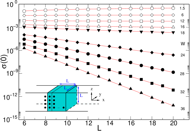
Figure 2: Finite size scaling of the DC conductivity calculated directly [5] within the Landauer Büttiker type geometry shown in the inset.

The good quality of the obtained conductivity data allows for tests of the various analytical predictions for the finite frequency behaviour. In particular, for $d>2$ dimensions we expect $\Delta\sigma=\sigma(\omega)-\sigma(0)\sim\omega^{(d-2)/2}$ in the metallic phase, $\sigma(\omega)\sim\omega^{(d-2)/d}$ at the metal-insulator transition, and $\sigma(\omega)\sim\omega^{2}$ far inside the insulating phase [6]. Figures 1 and 3 illustrate that for low frequency $\sigma(\omega)$ is indeed well described by a power law $\sigma(0)+C\,\omega^{\alpha}$. As expected, for samples with open boundary conditions (OBC) the extrapolated DC contribution $\sigma(0)$ is always zero, whereas for periodic (PBC) and anti-periodic (ABC) boundary conditions we observe a continuous metal-insulator transition at $W/t\approx 16$. As a further check we also calculated $\sigma(0)$ directly using a numerical Greens function approach within a Landauer Büttiker type geometry [5] and the finite size scaling ansatz $\sigma(0)=Le^{-L/\lambda}/(a+L)$ (cf. Fig. 2). Interestingly, within both approaches the resulting critical exponent for $\sigma(0)$ seems to be of the order of 2, larger than the expected $\nu\approx 1.57$, a puzzle which certainly requires further examination. Focussing on the exponent $\alpha$, our PBC and ABC data appears to be consistent with the analytic predictions, i.e., $\alpha\to 0.5$ for weak disorder, $\alpha\approx 1/3$ at the critical disorder, and eventually $\alpha\to 2$ for very strong disorder. Note, however, that for OBC $\alpha$ is a simple, monotonously increasing function of $W$. The above results show, that the new technique is a reliable numerical tool for large scale calculations of dynamical correlations functions.

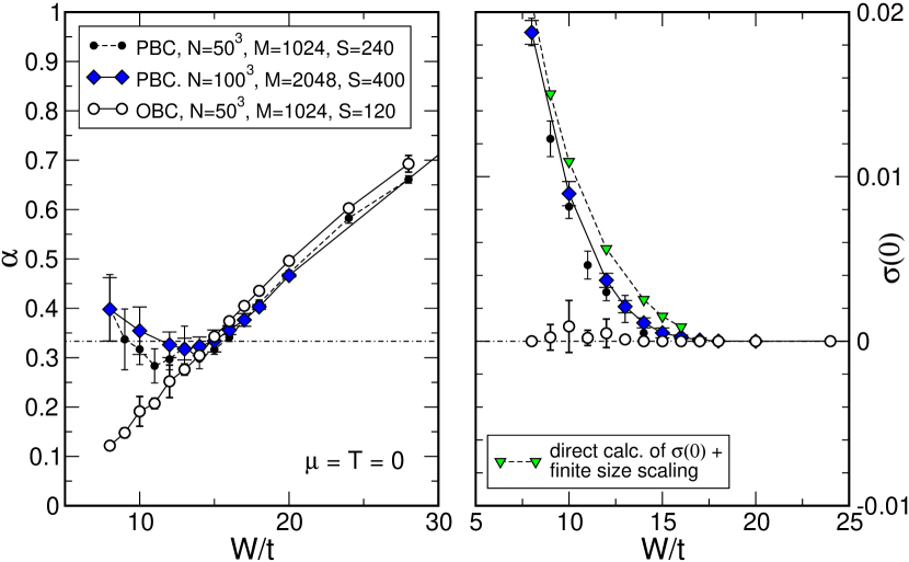
Figure 3: Exponent $\alpha$ and DC conductivity $\sigma(0)$ obtained from fits of the low-frequency conductivity to $\sigma(\omega)=\sigma(0)+C\,\omega^{\alpha}$ (vertical bars in Fig. 1 mark the underlying frequency range). Error bars are estimated by slightly varying $\mu\in[-0.05W,0.05W]$.

We acknowledge financial support by the Australian Research Council, calculations were performed at APAC Canberra, ac3 Sydney and NIC Jülich.

References

- [1] A. Weiße, Eur. Phys. J. B 40 (2004) 125.
- [2] P. W. Anderson, Phys. Rev. 109 (1958) 1492.
- [3] R. C. Albers, J. E. Gubernatis, Phys. Rev. B 17 (1978) 4487; A. Singh, W. L. McMillan, J. Phys. C 18 (1985) 2097; M. Hwang, A. Gonis, A. J. Freeman, Phys. Rev. B 35 (1987) 8974; P. Lambrianides, H. B. Shore, Phys. Rev. B 50 (1994) 7268; H. Shima, T. Nakayama, Phys. Rev. B 60 (1999) 14066.
- [4] R. N. Silver, H. Röder, Int. J. Mod. Phys. C 5 (1994) 935.
- [5] J. A. Vergés, Comp. Phys. Comm. 118 (1999) 71.
- [6] N. F. Mott, Adv. Phys. 16 (1967) 49; F. J. Wegner, Z. Phys. B 25 (1976) 327; R. Oppermann, F. Wegner, Z. Phys. B 34 (1979) 327; B. Shapiro, E. Abrahams, Phys. Rev. B 24 (1981) 4889; B. Shapiro, Phys. Rev. B 25 (1982) 4266.