Appearance of topological phases in superconducting nanocircuits

Abstract

We construct non-Abelian geometric transformations in superconducting nanocircuits, which resemble in properties the Aharonov-Bohm phase for an electron transported around a magnetic flux line. The effective magnetic fields can be strongly localized, and the path is traversed in the region where the energy separation between the states involved is at maximum, so that the adiabaticity condition is weakened. In particular, we present a scheme of topological charge pumping.

When an electron is transported in magnetic field around a closed loop, it acquires a phase equal to the magnetic flux through the surface spanned by the electron path. This phenomenon has been known as the Aharonov-Bohm effect for nearly half of a century AB . In the original paper the magnetic field forms a flux line, and electrons move in the region of zero field. Berry (1984) considered this phenomenon to be an early example of the geometric phases, which he described in a more general context. For each quantum system undergoing adiabatic cyclic evolution of its parameters we can find phase shifts acquired by its energy eigenstates. Apart from the dynamical factor, there is a contribution which depends only on the geometry of the path traversed in the parameter space (the parameters are time dependent, as they are varied throughout the process, but the explicit time dependence does not enter the expression for the Berry phase, which makes it geometric in nature). Berry gives also a formula for this phase in the form of an integral of an effective magnetic field (we will refer to this field as the “Berry field”) over a surface spanned by the path. This makes the similarity between geometric phases in arbitrary quantum system, and the Aharonov-Bohm scenario even closer: one can think of the Berry field as analogous to the real magnetic field; the parameter space corresponds then to the real position space. The Aharonov-Bohm effect in the original setting is, however, easier to observe than the Berry phase in general. The first reason is that in the former case there is no adiabaticity condition constraining the electron velocity, while in the latter the rate of the parameters’ variation should be much smaller than the inverse energy difference between the states involved. The second is that for strongly localized field any variation in the path of the electron does not affect the phase at all as long as the path encloses the flux line (this phase is thus topological). For the Berry phase, depending on the system, we encounter effective fields usually smoothly varying with the parameters, or even uniform, particularly for a spin-$1/2$ system, the phase is the flux of a monopole, or, in other words, the area spanned by the traversed loop on the unit sphere (see e.g. Berry (1984)). Fluctuations of externally controlled parameters first of all lead to dephasing of dynamical origin, but also smear the path, which affects the visibility of the effect even further.

Here we show that geometric phases can appear in quantum systems which are robust in the sense explained above: the effective magnetic field obtained from the Berry formula (the Berry field) is not necessarily a monopole (uniform in space) field, but can be strongly localized near the points of the lowest energy spacing between the states involved, and thus the geometric phases generated in the process can be topological. The field is suppressed in the region where the energy spacing is at maximum. This region is thus the most robust, as the fluctuations of the parameters do not change the geometric phases. Since the energy spacing is large in this region, the adiabaticity condition is weakened, and the path traversed relatively fast should give strong effects.

We find here the simplest, two-dimensional non-Abelian phases in the system considered in Ref. chola , but for a different range of the system parameters. This changes the picture substantially, as the topological properties of the phases become now evident (geometric phases in superconducting nanocircuits have been studied also in Falci et al. (2000); L. Faoro et al. (2003); in the earlier settings, however, the phases have not been proven to be topological). In our system the operational subspace is a twofold degenerate ground state, so that the dynamical contribution is just an overall phase factor, and the actual transformations are of purely geometric origin. Since the fields are localized, these transformations are topological in nature. Furthermore, we find a way to control the localization of the Berry field, as well as of the phase acquired while going around the region of enhanced field. The position of the peaks can be found from the parameter dependence of the spectrum; the degree of the localization reflects the deviation of the imaginary part of the Hamiltonian from zero. In the limit of completely real Hamiltonian, the Berry field is zero except for singular points, and the geometric phase can have only discreet values $\{-\pi,0,\pi\}$.

The system we consider (see Fig. 1) consists of two charge qubits makhlin coupled to each other via a dc SQUID (superconducting quantum interference device). The electrostatic energy of the system, including all the capacitances in the system, depends on the number of the Cooper-pairs on each island [denoted by $(n_{1},n_{2})$], and equals $E_{n1,n2}=E_{c1}(n_{g1}-n_{1})^{2}+E_{c2}(n_{g2}-n_{2})^{2}+E_{m}(n_{g1}-n_{1})(n_{g2}-n_{2})$. with $E_{c1}=4e^{2}C_{\Sigma 2}/2(C_{\Sigma 1}C_{\Sigma 2}-C_{m}^{2})$, and similarly for $E_{c2}$. Here $C_{\Sigma 1(2)}$ is the sum of all capacitances connected to the first (second) island. The inter-qubit electrostatic coupling $E_{m}=4e^{2}C_{m}/(C_{\Sigma 1}C_{\Sigma 2}-C_{m}^{2})$. The Josephson coupling $J^{(1)}=\sqrt{(J^{(1)}_{d}-J^{(1)}_{u})^{2}+4J^{(1)}_{u}J^{(1)}_{d}\cos^{2}(\pi\Phi_{1})}\exp[-i\psi(\Phi_{1})]$ (and similarly for $J^{(2)}$), where $\tan\psi(\Phi_{1})=(J^{(1)}_{d}-J^{(1)}_{u})/(J^{(1)}_{d}+J^{(1)}_{u})\tan\pi\Phi_{1}$ Tinkham . Here the couplings $J_{d}$, and $J_{u}$ correspond to the lower and upper junctions in the dc SQUIDs, which connect the qubits to their reservoirs. The upper junctions $J_{u}^{(1)}$, and $J_{u}^{(2)}$ are here replaced with another dc SQUID loops, which enables control over the symmetry of the big dc SQUIDs (the meaning of this technique is explained in more details in Ref. chola ). The important fact is that the Josephson coupling is real for $J_{u}=J_{d}$, and complex otherwise. Finally $J_{m}=J_{m}^{(0)}\cos\pi\Phi_{m}$ is the Josephson energy of the middle SQUID. The magnetic fluxes are here normalized to $\Phi_{0}=hc/2e$, the superconducting flux quantum.

Figure 1: (a) The system composed of two “charge qubits,” where the state is encoded in the number of Cooper pairs on the superconducting islands (black nodes), i.e. $n_{1}$, $n_{2}$. The voltages and magnetic fluxes can be controlled in a cyclic way in order to perform non-Abelian geometric transformations. (b) A simplified setup for topological charge pumping.

The Hamiltonian of the system reads

$$H = \sum_{n_{1},n_{2}}E_{n_{1},n_{2}}|n_{1},n_{2}\rangle\langle n_{1},n_{2}|-{1\over 2}\left(J_{1}|n_{1},n_{2}\rangle\langle n_{1}+1,n_{2}|\right.$$ (1)

$$+ J_{2}|n_{1},n_{2}\rangle\langle n_{1},n_{2}+1|+J_{m}|n_{1}+1,n_{2}\rangle\langle n_{1},n_{2}+1|$$

$$\left.+h.c.\right).$$

For the Josephson couplings switched off ($J_{1}=J_{2}=J_{m}=0$), the energy eigenstates are the charge states with their corresponding electrostatic energies. For the particular point $n_{g1}=n_{g2}=1/2$, the states $|\bar{0}\rangle\equiv|01\rangle$ and $|\bar{1}\rangle\equiv|10\rangle$ span twofold degenerate ground state. We construct the geometric transformations by choosing an appropriate closed path in the parameter space, which begins (and ends) at this point (and we refer to it as to the starting point). If the gate voltages $n_{g1}$ and $n_{g2}$ are close to $1/2$, only four states are relevant ($n_{1,2}=0,1$), and the calculation of the geometric transformations corresponding to given paths is straightforward.
In particular , if we keep the couplings $J_{1}=J_{m}=0$, while $J_{2}$ complex and finite, the states $|\bar{0}\rangle$ and $|\bar{1}\rangle$ belong to two decoupled subspaces of the Hilbert space. By varying adiabatically two parameters, e.g. $n_{g2}$ and $\Phi_{2}$ around a loop, we generate a phase shift between those states [$\exp(i\phi_{1}\sigma_{z}/2)$ in the basis $\{|\bar{0}\rangle,|\bar{1}\rangle\}$] equal to the difference of the Berry phases acquired by the states. The remaining independent parameter $n_{g1}$ is adjusted accordingly during the variation, so that the degeneracy in the ground state is maintained. Similarly for parameters specified by $J_{1}=J_{2}=J$ and $E_{01}=E_{10}$, the states $|+\rangle=(|\bar{0}\rangle+|\bar{1}\rangle)/\sqrt{2}$ and $|-\rangle=(|\bar{0}\rangle-|\bar{1}\rangle)/\sqrt{2}$ belong to decoupled subspaces, and the geometric phase shift between them again equals to the difference of their Berry phases. In the latter case, however, the corresponding transformation is $\exp(i\phi_{2}\sigma_{x}/2)$, so that the two transformations generate a non-Abelian group of (all) unitary transformations within the subspace $\{|\bar{0}\rangle,|\bar{1}\rangle\}$.

Let us now recall the original Berry formula for the geometric phase. The Hamiltonian is smoothly varied in time with its parameters, $H[R(t)]$, and for each point $R(t)$ of the parameter space its eigenstates are $|n[R(t)]\rangle$ with the energies $E_{n}[R(t)]$. The geometric phase corresponding to the path $C$ in the parameter space, acquired by the state $|n\rangle$, equals then

$$\gamma_{n}(C)=-\int_{S(C)}dS\cdot V_{n}(R),$$ (2)

where the integral is evaluated over the surface spanned by $C$ of the effective magnetic (Berry) field

$$V_{n}(R)=\Im\sum_{m\neq n}{\langle n|\nabla_{R}H|m\rangle\times\langle m|\nabla_{R}H|n\rangle\over(E_{m}(R)-E_{n}(R))^{2}}.$$ (3)

The energy difference in the denominator makes it possible to predict the regions of suppressed and enhanced field. Let us consider the spectral characteristics of our system. In Fig.2(a) we see exemplary diagram of the ground-state charging energies. If we move along the borders between the cells, the ground state remains twofold degenerate. In Fig.2(b) the spectrum corresponding to the thick line in (a) is plotted as the function of $n_{g2}$.

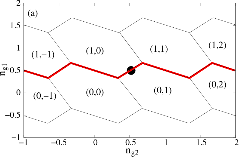
Figure 2: (a) Ground state charging diagram and (b) electrostatic energies corresponding to the thick line in (a). The black node denotes hereafter the starting point. Inset: nonzero Josephson coupling mixes the states so that there is an avoided level crossing near the “triple points” in (a).

If we now want to perform a phase shift between the states $|\bar{0}\rangle$ and $|\bar{1}\rangle$, we switch the coupling $J_{2}$ to a finite value. The coupling will strongly mix the states near the points of crossing with the first excited state, as shown in the right inset of Fig. 2(b). However, even for finite coupling, the minimum in the energy separation between the ground state, and the first excited state will correspond to $n_{g2}$ of the triple points in Fig.2(a). For these points, the spacing further depends on $|J_{2}|$, which is tuned by the flux $\Phi_{2}$ and has a minimum value for $\Phi_{2}=1/2+k$ and maximum for $\Phi_{2}=k$, $k$ being an integer. The same discussion applies to the second transformation, $\exp(i\phi_{2}\sigma_{x}/2)$. Assuming for simplicity that the design is symmetric (characteristics of the charge qubits are identical), we expect minimum spacing for $\Phi\equiv\Phi_{1}=\Phi_{2}=1/2+k$, and $n_{g}\equiv n_{g1}=n_{g2}$ corresponding to the triple points ($\Phi_{m}$ is in this case used to maintain the degeneracy in the ground state). On the other hand, the field should be strongly suppressed (and it is, as shown below) in the region of maximum spacing between the ground state and the first excited state. Since the aforementioned transformations are performed by varying both, voltages and fluxes, which tune the electrostatic, and the Josephson energies, the optimal system should have the characteristic Josephson, and electrostatic energies are of comparable magnitude. [In Ref.chola the transformations are constructed in the charge regime (electrostatic energies are much bigger than the Josephson energies) and the range of parameters considered there lies between the minima of energy spacing, so that the Berry field seems to be smooth and weak.]

In Fig.3(a) we see the difference in energy between the first excited and the ground state (for $J_{m}=J_{1}=0$, $E_{c1}=E_{c2}=E_{m}$, $J_{d}^{(2)}/E_{m}=1/2$, and $J_{u}^{(2)}/E_{m}=2/5$), as the function of $n_{g2}$ and $\Phi_{2}$. The gate voltage $n_{g1}$ is adjusted so that the ground state remains degenerate. In Fig.3(b) we see the Berry field for the same range of parameters. The peak position corresponds indeed to the minimum in the energy separation. The most robust paths should be placed far from the peak, and at maximum energy separation (so that the adiabaticity condition is weak). In our case the optimal path is the border of the rectangle $(n_{g2},\Phi_{2})\in[0,0.5]\times[0,1]=S$ [actually the peaks (and dips) form a lattice in the $n_{g2}$-$\Phi_{2}$ plane, so that the most robust paths are borders of all Wigner-Seitz primitive cells of the lattice].

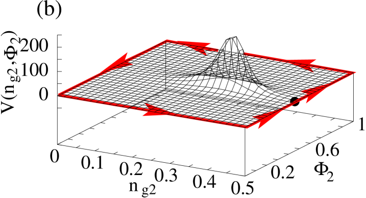
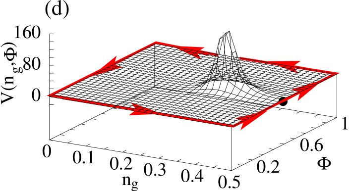
Figure 3: (a) Parameter-dependent spectrum, and (b) effective magnetic field. The minimum in the energy spacing corresponds to the maximum in the field strength. Variation of the parameters around the peak results in a phase shift between $|\bar{0}\rangle$ and $|\bar{1}\rangle$. (c), (d) Similar characteristics corresponding to the phase shift between $|+\rangle$ and $|-\rangle$. The contours denote the most robust paths.

One turn along the path produces a phase shift $\exp(i\phi_{1}\sigma_{z}/2)$, where

$$\phi_{1}=\int_{S}dn_{g2}d\Phi_{2}V(n_{g2},\Phi_{2}).$$ (4)

Similarly, for $J_{1}=J_{2}=J$, and $n_{g}=n_{g1}=n_{g2}$ (for simplicity we assume that the qubits are identical) we vary $n_{g}$ and $\Phi=\Phi_{1}=\Phi_{2}$ to perform the transformation $\exp(i\phi_{2}\sigma_{x}/2)$ ($\Phi_{m}$ is tuned to maintain the degeneracy in the ground state), where

$$\phi_{2}=\int_{S}dn_{g}d\Phi V(n_{g},\Phi).$$ (5)

The field $V(n_{g},\Phi)$, for $J_{d}^{(1),(2)}/E_{m}=1/2$ and $J_{u}^{(1),(2)}/E_{m}=2/5$, is shown in Fig.3(d), and the spectral characteristics for the same range of parameters in Fig.3(c). The optimal path is here again the border of the rectangle $(n_{g},\Phi)\in[0,0.5]\times[0,1]=S$ or of any other Wigner-Seitz cell of the lattice.

The phase shift acquired during one cycle can be controlled by the strength of the Josephson couplings $J_{u}^{(1),(2)}$, which are tuned by varying the fluxes through the small SQUID loops. Let us illustrate this effect for the phase shift $\phi_{1}$. In Fig.4(a) we see the phase acquired during one cycle as the function of $J_{u}/J_{d}$. The phase shift increases as the asymmetry of the right SQUID is reduced, and tends to the value $\pi$ (and for $J_{u}/J_{d}=1$ is exactly $\pi$ as explained below). In Fig.4(b) we see that together with reduction of the asymmetry of the SQUID, the width of the peaks tends to zero. Thus the effect seems to be amplified together with enhanced localization of the field.

Figure 4: Dependence of the phase acquired during one turn around the region of enhanced field (a) and localization of the field (b) as functions of $J_{u}/J_{d}$.

Simple reasoning shows that for symmetric SQUIDs ($J_{u}=J_{d}$) the effective field is zero, except for singular points. Moreover, loops enclosing an odd number of these singularities correspond to the phase shifts $\phi_{1}=\pm\pi$ and $\phi_{2}=\pm\pi$. Indeed, for symmetric SQUIDs the Hamiltonian in Eq.(1) is real. The Berry field is, as seen from Eq.(3) zero, unless there is a crossing in the energy difference between the ground state and the first excited state. Such singularities are points of zero Josephson couplings ($\Phi_{1}=\Phi_{2}=\Phi_{m}=1/2$) and can be easily identified as the triple points in the charging diagram (see Fig. 2). Depending on the transformation we want to perform, one of the degenerate lowest states ($|\bar{0}\rangle$ or $|\bar{1}\rangle$ and $|+\rangle$ or $|-\rangle$) is for each singular point decoupled from the first excited state, and the Berry phase will be zero for this state, even if the path encloses the singularity. The complementary state, however, is coupled [in the sense that the numerator in Eq.(3) is nonzero] to the excited state, and the phase shift will be nontrivial. As only two states are involved in the transformation, we can now use the spin-$1/2$ picture. The real Hamiltonian $H=-B\cdot\sigma/2$ is parametrized by the $B$-field which has only $x$ and $z$ nonvanishing components, so that each path lies in the plane containing degeneracy. Cyclic evolution of the parameters corresponds to solid angles either $0$, when the loop does not enclose the degeneracy, or $\pm 2\pi$, when it does. The corresponding Berry phase is thus either $0$ or $\pm\pi$ (see also Berry (1984)). Applying the result to our system we see that the phases $\phi_{1}$ and $\phi_{2}$ can have only values $0$ or $\pm\pi$, so that the resulting non-trivial transformations within the subspace $\{|\bar{0}\rangle,|\bar{1}\rangle\}$ are $\pm\sigma_{z},\pm\sigma_{x}$.

The latter transformation is a topological charge pumping. This can be the easiest effect to observe experimentally as it requires a simplified setup [see Fig. 1(b)], with symmetric SQUID loops only, a single voltage source, and a single current line generating equal control fluxes $\Phi_{1}$ and $\Phi_{2}$ (assuming identical qubits). Let us estimate the rate of the dynamical dephasing for this scheme. Fluctuations of the fluxes $\Phi_{1}=\Phi_{2}$, and of the gate voltage $n_{g}$ do not violate the constraints that we put on the parameters. Thus the most important source of errors is in this case the fluctuating flux $\Phi_{m}$. Since we are interested in the degenerate subspace only, we apply here the formula for the dephasing rate in the environment-dominated regime, $\Gamma_{\phi}\approx 2\pi\alpha k_{B}T/\hbar$ mss . Here $\alpha$ is the constant describing the strength of the system-environment coupling. At the starting point, where the dependence of $J_{m}$ on the flux is strongest, the dephasing rate will be at maximum, and we take this value as our estimate. At this point $\alpha=R_{K}(MJ_{m}^{0}\pi/\Phi_{0}^{2})^{2}/4R_{I}$, where the resistance of the external circuit inducing the flux, $R_{I}$, is typically of the order of $100\Omega$. $R_{K}\approx 25.8\mbox{k}\Omega$ is the quantum resistance, and $M\approx 0.1-0.01$nH is the mutual inductance between the SQUID and the control circuit. The dephasing rate should be compared to the mean energy separation between the excited and the ground state $\bar{\omega}_{e\rightarrow g}$, which constraints the time in which the loop is traversed. Then for $J_{m}^{0}\approx 1$K and at $T=20$mK we obtain $\Gamma_{\phi}/\bar{\omega}_{e\rightarrow g}\approx 10^{-5}-10^{-3}$. At optimal design there should be thus much space left to both satisfy the adiabaticity condition and perform many charge pumping cycles within the time $\Gamma_{\phi}^{-1}$.

To summarize, the results presented here prove the possibility to perform robust geometric transformations in quantum systems by identifying points of localized effective magnetic field. The resulting procedure resembles the original setting of the Aharonov-Bohm effect. In this particular system the geometric phases will be accompanied by dephasing of dynamical origin, as the degeneracy of the ground state is controlled by external parameters. However, the weak adiabaticity condition on one hand and dominant role of the Berry field from the interior of the enclosed region on the other make it possible to traverse the paths quickly (and generate large phase shifts), before the dephasing destroys the visibility of the effect.

The author thanks Yu. Makhlin, R. W. Chhajlany, and R. Fazio for stimulating discussions and comments. This work was supported by the DFG-Schwerpunktprogramm “Quanten-Informationsverarbeitung”, EU IST Project SQUBIT, and EC Research Training Network.

References

- (1) Y. Aharonov and D. Bohm, Phys. Rev. 115, 485 (1959),
- Berry (1984) M. V. Berry, Proc. R. Soc. London, Ser. A 392, 45 (1984)
- (3) M. Cholascinski, Phys. Rev. B 69, 134516 (2004),
- Falci et al. (2000) G. Falci, R. Fazio, G. M. Palma, J. Siewert, and V. Vedral, Nature (London) 407, 355 (2000).
- L. Faoro et al. (2003) L. Faoro, J. Siewert, and R. Fazio, Phys. Rev. Lett. 90, 028301 (2003).
- (6) Yu. Makhlin, G. Schön, and A. Shnirman, Nature (London) 398, 305 (1999),
- (7) M. Tinkham, Introduction to Superconductivity, 2nd ed. (McGraw-Hill, New York, 1996).
- (8) Y. Makhlin, G. Schön, A. Shnirman, Rev. Mod. Phys. 73, 357 (2001).