The Totally Asymmetric Simple Exclusion Process with Langmuir Kinetics

Abstract

We discuss a new class of driven lattice gas obtained by coupling the one-dimensional totally asymmetric simple exclusion process to Langmuir kinetics. In the limit where these dynamics are competing, the resulting non-conserved flow of particles on the lattice leads to stationary regimes for large but finite systems. We observe unexpected properties such as localized boundaries (domain walls) that separate coexisting regions of low and high density of particles (phase coexistence). A rich phase diagram, with high an low density phases, two and three phase coexistence regions and a boundary independent “Meissner” phase is found. We rationalize the average density and current profiles obtained from simulations within a mean-field approach in the continuum limit. The ensuing analytic solution is expressed in terms of Lambert $W$-functions. It allows to fully describe the phase diagram and extract unusual mean-field exponents that characterize critical properties of the domain wall. Based on the same approach, we provide an explanation of the localization phenomenon. Finally, we elucidate phenomena that go beyond mean-field such as the scaling properties of the domain wall.

I Introduction

Many natural phenomena driven by some external field or containing self-propelled particles evolve into stationary states carrying a steady current. Such states are characterized by a constant gain or loss of energy, which distinguishes them from thermal equilibria. Examples range from biological systems like ribosomes moving along m-RNA or motor molecules “walking” along molecular tracks to ions diffusing along narrow channels, or even cars proceeding on highways. In order to elucidate the nature of such non-equilibrium steady states a variety of driven lattice gas models have been introduced and studied extensively Schmittmann and Zia (1995). Here we focus on one-dimensional (1D) models, where particles preferentially move in one direction. In this context, the Totally Asymmetric Simple Exclusion Process (TASEP) has become one of the paradigms of non-equilibrium physics (for a review see Refs. Spohn (1991); Derrida and Evans (1997); Mukamel (2000); Schütz (2001)). In this model a single species of particles is hopping unidirectionally and with a uniform rate along a 1D lattice. The only interaction between the particles is hard-core repulsion, which prevents more than one particle from occupying the same site on the lattice; see Fig. 1.

It has been found that the nature of the non-equilibrium steady state of the TASEP depends sensitively on the boundary conditions. For periodic boundary conditions the system reaches a steady state of constant density. Interestingly, density fluctuations are found to spread faster than diffusively van Beijeren et al. (1985). This can be understood by an exact mapping Meakin et al. (1986) to a growing interface model, whose dynamics in the continuum limit is described in terms of the KPZ equation Kardar et al. (1986) and its cousin, the noisy Burgers equation Forster et al. (1977). In contrast to such ring systems, open systems with particle reservoirs at the ends exhibit phase transitions upon varying the boundary conditions Krug (1991). This is genuinely different from thermal equilibrium systems where boundary effects usually do not affect the bulk behavior and become negligible if the system is large enough. In addition, general theorems do not even allow equilibrium phase transitions in one-dimensional systems at finite temperatures (if the interactions are not too long-range) Landau and Lifshitz (1980).

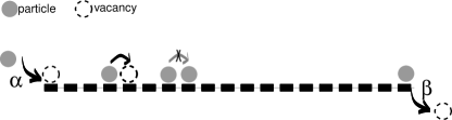
Figure 1: Illustration of the Totally Asymmetric Simple Exclusion Process with open boundaries. The entrance and exit rates at the left and right end of the one-dimensional lattice are given by $\alpha$ and $\beta$, respectively.

Yet another difference between equilibrium and non-equilibrium processes can be clearly seen on the level of its dynamics. If transition rates between microscopic configurations are obeying detailed balance the system is guaranteed to evolve into thermal equilibrium . Systems lacking detailed balance may still reach a steady state, but at present there are no universal concepts like the Boltzmann-Gibbs ensemble theory for characterizing such non-equilibrium steady states. In most instances one has to resort to solving nothing less than its full dynamics. It is only recently, that exact (non-local) free energy functionals for driven diffusive systems have been derived Derrida et al. (2001, 2002).

This has to be contrasted with dynamic processes such as the adsorption-desorption kinetics of particles on a lattice coupled to a bulk reservoir (“Langmuir Kinetics”, LK), see Fig. 2. Here, particles adsorb at an empty site or desorb from an occupied one. Microscopic reversibility demands that the corresponding kinetic rates obey detailed balance such that the system evolves into an equilibrium steady state, which is well described within standard concepts of equilibrium statistical mechanics. If interactions between the particles other than the hard-core repulsion are neglected, the equilibrium density is solely determined by the ratio of the two kinetic rates Fowler (1936), as given by the Gibbs ensemble.

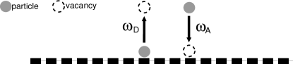
Figure 2: Illustration of Langmuir kinetics. $\omega_{A}$ and $\omega_{D}$ denote the local attachment and detachment rates.

The TASEP and LK can be considered as two of the simplest paradigms which contrast equilibrium and non-equilibrium dynamics and stationary states. Langmuir kinetics evolves into a steady state well described in terms of standard concepts of equilibrium statistical mechanics. Driven lattice gases such as the TASEP evolve into a stationary non-equilibrium state carrying a finite conserved current. Whereas such non-equilibrium steady states are quite sensitive to changes in the boundary conditions, equilibrium steady states are very robust to such changes and dominated by the bulk dynamics. In the TASEP the number of particles is conserved in the bulk of the one-dimensional lattice. It is only through the particle reservoirs at the system boundaries that particles can enter or leave the system. In LK particle number is not conserved in the bulk. Particles can enter or leave the system at any site. Depending on whether we consider a canonical or grand canonical ensemble the lattice is connected to a finite or infinite particle reservoir. Unlike the steady state of the TASEP, the equilibrium steady state of LK does not have any spatial correlations.

Combining both of these processes may at first sight seem a trivial exercise since one might expect bulk effects to be predominant in the thermodynamic limit. This is indeed the case for attachment and detachment rates, $\omega_{A}$ and $\omega_{D}$, which are independent of system size $N$. For large but finite systems interesting effects can only be expected if the kinetics from the TASEP and LK compete. Then, as we have shown recently Parmeggiani et al. (2003), novel behavior different from both LK and the TASEP appears. In particular, one observes phase separation into a high and low density domain for an extended region in parameter space.

When should one expect competition between bulk dynamics (LK) and boundary induced non-equilibrium effects (TASEP)? Let’s consider the following heuristic argument. A given particle will typically spend a time $\tau\sim 1/\omega_{D}$ on the lattice before detaching. During this “residence” time the number of sites $n$ explored by the particle is of the order of $n\sim\tau$. Hence, for fixed $\omega_{D}$, the fraction $n/N\sim 1/(\omega_{D}N)$ of sites visited by a particle during its walk on the lattice would go to zero as $N\to\infty$. Only if we introduce a “total” detachment rate by $\Omega_{D}=N\omega_{D}$ and keep it constant instead of $\omega_{D}$ as $N\to\infty$ will the particle travel a finite fraction of the total lattice size. Similar arguments show that a vacancy visits an extensive number of sites until it is filled by attachment of a particle if $\omega_{A}$ scales to zero as $\omega_{A}=\Omega_{A}/N$ with a fixed “total” attachment rate $\Omega_{A}$. In other words, competition will be expected only if the particles live long enough such that their internal dynamics or the external driving force transports them a finite fraction along the lattice before detaching. Then, particles spend enough time on the lattice to “feel” their mutual interaction and, eventually, produce collective effects. In summary, competition between bulk and boundary dynamics in large systems ($N\gg 1$) is expected if the kinetic rates $\omega_{A}$ and $\omega_{D}$ decrease with increasing system size $N$ such that the total rates $\Omega_{A}$ and $\Omega_{D}$ with

$$\Omega_{A}=\omega_{A}N\,, \quad\Omega_{D}=\omega_{D}N$$ (1)

are kept constant with $N$.

The competition between boundary and bulk dynamics is a physical process that has, to our knowledge, not yet been studied in the context of driven diffusive systems. In previous models emphasis was put on the analysis of boundary induced phenomena in driven gases of mono- or multi-species of particles Lahiri and Ramaswamy (1997); Lahiri et al. (2000); Evans et al. (1998); Mukamel (2000); Schütz (2001, 2003), in presence of interactions (see e.g. Ref. Katz et al. (1983, 1984)), disorder Tripathy and Barma (1997, 1998) or local inhomogeneities Kolomeisky (1998); Mirin and Kolomeisky (2003), particles with sizes larger than the lattice spacing Lakatos and Chou (2003); Shaw et al. (2003), lattices with different geometries (e.g. multi-lanes lattice gases Popkov and Peschel (2001)), or systems in presence of several conservation laws (for a review see e.g. Ref. Schütz (2003)).

In this manuscript we explore the consequences of particle exchange with a reservoir along the track (LK) on the stationary density and current profiles and the ensuing phase diagram of the TASEP. A short account of our ideas has been given recently Parmeggiani et al. (2003), where we have introduced the model and have shown how our Monte Carlo results can be rationalized on the basis of a mean-field theory, which we also solved analytically. The purpose of the present manuscript is to give a complete and comprehensive discussion of the topic. We will present results from Monte-Carlo results for the full parameter range of the model including the particular case where on- and off-rates equal each other, which were left out in our short contribution Parmeggiani et al. (2003) due to the lack of space. In addition, we will give the full reasoning for the derivation and analytical solutions of our mean-field theory. Here, additional insight is gained by identifying a branching point that explains all the features of the density profiles and phase diagram analytically. In particular, we show that a new critical point organizes the topology of the diagram and leads to unexpected phenomena already briefly discussed in Ref. Parmeggiani et al. (2003). In a recent work, Evans et al. Evans et al. (1998) have rephrased the mean-field analysis first given in Ref. Parmeggiani et al. (2003) and reproduced some of our results. The mean-field equations are, however, left in their implicit form and thus miss the interesting features we will obtain from the identification of a branching point.

These effects differ from those known in reference models of equilibrium and non-equilibrium statistical mechanics like LK and the TASEP. Indeed, the coupling between the TASEP and LK, as is was introduced above, produces new phenomena and extends the interest toward systems which break conservation law in a non-trivial way. As we shall see in the next Section, these features emerge already at level of properties of the microscopic dynamics in configuration space described by the master equation.

Recently a variant of our model has been suggested by Popkov et al.  Popkov et al. (1998). Upon supplementing the Katz-Lebowitz-Spohn model by Langmuir kinetics and analyzing it within the mean-field approach similar to Parmeggiani et al. (2003), an even richer scenario for the stationary density profile is obtained that includes the emergence of localized downward domain walls and the appearance of several ’shocks’ separating three distinct phases. It is also noted in Ref. Popkov et al. (1998) that in general it may be important to replace the mean-field current by the exact current in the stationary state.

In addition to its fundamental importance for non-equilibrium physics in general, competition between bulk dynamics and boundary effects are ubiquitous in nature, in particular biological phenomena. The TASEP has actually been introduced in the biophysical literature as a model mimicking the dynamics of ribosomes moving along a messenger RNA chain MacDonald et al. (1968); for generalizations of these studies, see the recent work in Refs. Shaw et al. (2003); Chou (2003). Also some aspects of intracellular transport show close resemblance to our model. For example, processive molecular motors advance along cytoskeletal filaments while attachment and detachment of motors between the cytoplasm and the filament occur Howard (2001). Typically kinetic rates are such that these motors walk a finite fraction along the molecular track before detaching. This falls well into the regime where we expect novel stationary states. Recently, it has been shown that such dynamics can be relevant for modeling the filopod growth in eukaryotic cells produced by motor proteins interacting within actin filaments Kruse and Sekimoto (2002). Finally, our model could also be relevant for studies of surface-adsorption and growth in presence of biased diffusion or for traffic models with bulk on-off ramps Chowdhury et al. (2000).

Since our paper contains a rather comprehensive discussion of the topic, we will give a detailed outline to provide the reader with some guidance through the analysis. In Section II we define the model by its dynamic rules and make a connection to its stochastic dynamics on a network. Though the relation between stochastic dynamics and networks is interesting to fully understand the peculiar features of the model introduced by the combination of conserved dynamics and on/off kinetics, it may be skipped for the first reading. We then present the problem in terms of a Fock space formulation and discuss the symmetries of the model, both key features for the subsequent formulation of the mean-field theory. In Section III we briefly discuss some technical details of the Monte-Carlo simulation. Then follows a key section of the manuscript, a detailed development of the mean-field approximation and the resulting “Burgers”-like equations in the continuum limit. Here we also discuss a series of features of these equations which will turn out to be crucial for the understanding of the ensuing density and current profiles.

In Sect. IV an analytic solution of the continuum equations is derived and compared to simulation results. We start the discussion for the special case that on- and off-rates are identical. Though simpler to analyze, this case is somewhat artificial as it requires a fine-tuning of the on- and off-rates. Generically, one expects on- and off-rates to differ. Then the mathematical analysis becomes significantly more complex. We are still able to give an explicit analytical solution in terms of so-called Lambert functions, which allows us to identify a branching point that explains all the features of the density profiles and phase diagram analytically. In particular, we find a special point that organizes the topology of the diagram. In Sect. V we discuss the properties of the domain wall characterizing the phase coexistence upon changes of the model parameters. In particular, we show that in the vicinity of the special point mentioned above the domain wall exhibits non-analytic behavior similar to a critical point in continuous phase transitions. We derive the critical exponents and the scaling related to the amplitude and position of the domain wall. A conclusion, Sect. VI, summarizes our results and provides additional arguments on the phenomenon of phase coexistence. Last, we discuss some discrepancies between the mean-field approach and the simulation results and discuss a possible reconciliation.

II The Model

In this Section we are going to describe the model in some detail. We will also put it into the context of network theories. This will help us to pinpoint the differences between the TASEP and LK dynamics and show how a model combing both aspects will lead to novel phenomena. Finally, we briefly review the key ideas of the Fock space formulation of stochastic particle dynamics. In later chapters this formulation will be used for an analytic discussion of the model.

II.1 Definition of the dynamic rules

In the microscopic model we consider a finite one-dimensional lattice with sites labeled $i\!=\!1,...,N$ (see Fig. 3) and lattice spacing $a=L/N$, where $L$ is the total length of the lattice. The site $i=1$ ($i=N$) defines the left (right) boundary, while the collection $i\!=\!2,...,N-1$ is referred to as the bulk.

The microscopic state of the system is characterized by a distribution of identical particles on the lattice, i.e. by configurations ${\cal C}=\{n_{i=1,..N}\}$, where each of the occupation numbers $n_{i}$ is equal either to zero (vacancy) or one (particle). We impose a hard core repulsion between the particles, which implies that a double or higher occupancy of sites is forbidden in the model. The full state space then consists of $2^{N}$ configurations.

The statistical properties of the model are given in terms of the probabilities ${\cal P}({\cal C},t)$ to find a particular configuration ${\cal C}=\{n_{i}\}$ at time $t$. We consider the evolution of the probabilities ${\cal P}$ described by a master equation:

$$\frac{d{\cal P}({\cal C},t)}{dt}=\sum_{{\cal C^{\prime}}\neq{\cal C}}\Big{[}{\cal W}_{{\cal C^{\prime}}\to{\cal C}}{\cal P}({\cal C^{\prime}},t)-{\cal W}_{{\cal C}\to{\cal C^{\prime}}}{\cal P}({\cal C},t)\Big{]}\,.$$ (2)

Here, ${\cal W}_{{\cal C}\to{\cal C^{\prime}}}$ is a non-negative transition rate from configuration ${\cal C}$ to ${\cal C^{\prime}}$. As usual, master equations conserve probabilities. The microscopic processes connecting two subsequent configurations are local in configuration space. Out of the possible $2^{N}\times 2^{N}$ transitions, we consider only the following elementary steps connecting neighboring configurations:

• at the site $i\!=\!2,..,N-1$ a particle can jump to site $i+1$ if unoccupied with unit rate;

• at the site $i=1$ a particle can enter the lattice with rate $\alpha$ if unoccupied;

• at the site $i=N$ a particle can leave the lattice with rate $\beta$ if occupied.

Additionally, in the bulk we assume that a particle:

• can leave the lattice with site-independent detachment rate $\omega_{D}$;

• can fill the site (if empty) with a rate $\omega_{A}$ by attachment.

Processes $A)$ to $C)$ constitute a totally asymmetric simple exclusion process with open boundaries Derrida and Evans (1997); Mukamel (2000); Schütz (2001), while processes $D)$ and $E)$ define a Langmuir kinetics Fowler (1936). We have taken the attachment and detachment rates to be independent of the particle concentration in the reservoir, i.e. we have assumed that the Langmuir kinetics on the lattice is reaction and not diffusion limited. The effect of diffusion in confined geometry has been studied in Ref. Klumpp and Lipowsky (2003). A schematic graphical representation of the resulting totally asymmetric exclusion model with Langmuir kinetics Parmeggiani et al. (2003) is given in Fig. 3.

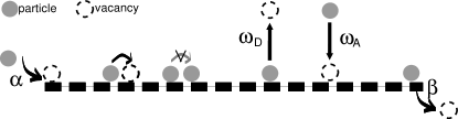
Figure 3: Schematic drawing of the totally asymmetric simple exclusion process with bulk attachment and detachment Parmeggiani et al. (2003). The entrance and exit rates at the left and right end of the one-dimensional lattice are given by $\alpha$ and $\beta$, respectively; $\omega_{A}$ and $\omega_{D}$ denote the local attachment and detachment rates.

Once we know the dynamic rules of the stochastic process, one may introduce the notion of neighboring configurations for ${\cal C}$ and ${\cal C^{\prime}}$, if they differ only by a small fraction (${\cal O}(1/N)$) of the corresponding occupation numbers. This naturally leads us to a reinterpretation of the dynamics in terms of networks as described in the following subsection.

II.2 Stochastic dynamics and networks

The Markovian dynamics of the system can be represented in terms of a network (graph), where the configurations of the stochastic process correspond to the nodes (vertices) of the network. Each transition allowed by the dynamics is represented as a directed link (edge), and weighted by the corresponding transition rate which can be read off from the dynamic rules $A)-E)$. Due to the local dynamics the network is very dilute. A given node in the network is connected to a maximum number $O(N)$ of nearby configurations. Nevertheless, any configuration can still be reached from any point within the network. In other words the network is connected and does not break into disjunct pieces. In addition, every node has at least one ingoing and one outgoing link. This guarantees that the system is ergodic, at least as long as $N$ is finite, and all states are recurrent Shiryaev (1995).

On such a network a distance between two different configurations can be defined as the minimal number of steps required to connect them. Note that the “architecture” of the network corresponding to a pure TASEP is very different from a pure LK; see Fig. 4 for an illustration.

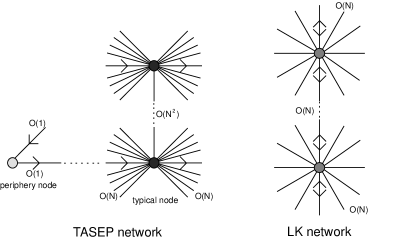
Figure 4: Illustration of the network architecture corresponding to the totally asymmetric simple exclusion process (TASEP) and Langmuir kinetics (LK).

The TASEP network is characterized by large fluctuations in the connectivity. Take for example the completely filled configuration. This state can only be left if the particle at the right end of the lattice is ejected from the system. Similarly, a configuration described by a step function $n_{i}=\Theta(x_{i}-x_{0})$ with a completely filled lattice to the left and a completely empty lattice to the right of $x_{0}$ can only be left by a single process where the rightmost particle is hopping forward. We call such and similar states “periphery states” since they are linked to the rest of the network by a single or only a few outgoing and ingoing links. This is to be contrasted with “typical states” for a given density, where particles are more or less randomly distributed over the lattice. Then, the conditional probability that an empty site is in front of a filled site will be finite. In other words, there will be an extensive number of pairs $(1,0)$ on the lattice. This implies that a typical state will be connected with an extensive number $O(N)$ of directed ingoing and outgoing links to other nodes in the network. Similarly, the shortest path connecting two non-neighboring configurations has a broad length distribution. Given two randomly chosen sequences of occupation numbers $n_{i}=0$ and $n_{i}=1$ (i.e. nodes) one has to ask, how many local moves of the type A) to C) (i.e. links) are needed to transform one sequence into the other. In general, there will be a distribution of paths connecting these nodes. The shortest connection may be only a few links, if local rearrangements of particles are sufficient for matching the microscopic configurations. It seems plausible that this is the case for such microscopic configurations, whose coarse-grained density profiles are identical or at least very similar. If the spatial profiles of the coarse-grained densities corresponding to the two configurations differ significantly, one expects $O(N^{2})$ local rearrangements to be necessary for matching the microscopic configurations. This is simply a consequence of particle conservation in the bulk. For example, to completely empty a totally filled state obviously requires $O(N^{2})$ steps. In addition, distances between two configurations in a TASEP network can also be highly asymmetric. Consider a configuration ${\cal C}$ corresponding to a node at the periphery of the network connected to a configuration ${\cal C^{\prime}}$. Then the corresponding reverse step does not exist, and in order return to the configuration ${\cal C}$ one has to make a large loop in configuration space. In summary, a network corresponding to TASEP contains only directed links. A characteristic feature is its heterogeneity in the connectivity of nodes and distances between nodes. The network contains loops, many of which may be very long due to the conservation law in the bulk.

This has to be contrasted with the architecture of a network corresponding to LK. Here, the connectivity of all nodes is independent of the particular configuration. Since each occupation number $n_{i}$ at a given site $i$ can be independently changed, the number of links outgoing from a node is simply $N$. To each outgoing link there is an ingoing link with weights related by detailed balance. Moreover, any two configurations can be reached by at most $N$ transitions. Since there is no conservation law, only local moves (particle attachment or detachment) are necessary. The distance of two configurations (along the shortest path) in a LK network is $d({\cal C},{\cal C^{\prime}})=\sum_{i=2}^{N-1}|n_{i}-n_{i}^{\prime}|$ . Since the order of the necessary attachment and detachment processes is irrelevant the number of such shortest paths is highly degenerate, and depends only on the distance as $d!$. In summary, the LK network is not directed, very homogeneous, highly connected and contains many loops of all size.

An important distinction between LK and the TASEP can be clearly seen if one compares the nature of the corresponding stationary states. Langmuir kinetics has a solution described in terms of the thermodynamic equilibrium distribution:

$${\cal P}({\cal C})=\frac{K^{|{\cal C}|}}{(K+1)^{N-2}}\,.$$ (3)

Here $|{\cal C}|\equiv\sum_{i=2}^{N-1}n_{i}$ is the number of occupied sites in the bulk and $K=\omega_{A}/\omega_{D}$ is the binding constant . Note that the equilibrium distribution of LK can be characterized by a Boltzmann weight upon introducing an effective Hamiltonian ${\cal H}=-k_{B}T\sum_{i=2}^{N-1}n_{i}\ln K$. The case $K=1$ has an interesting topological interpretation since the links in the LK network loose their directionality and the effective Hamiltonian ${\cal H}$ evaluates to $0$.

In contrast, the totally asymmetric exclusion process does not satisfy the detailed balance condition

$${\cal W}_{\,{\cal C^{\prime}}\to{\cal C}}~{}{\cal P}({\cal C^{\prime}})={\cal W}_{\,{\cal C}\to{\cal C^{\prime}}}~{}{\cal P}({\cal C})\,,$$

and evolves into a non-equilibrium steady state. Actually, if one would assume detailed balance along a closed directed loop in the TASEP network, one would be lead to the conclusion that all probabilities along the path have to be zero. This, in turn, would contradict the ergodicity of the finite system.

The network analogy discussed above can be used to understand why a stochastic dynamics combining the totally asymmetric exclusion process and Langmuir kinetics is interesting and show a range of novel features not contained in the TASEP or LK alone. We have seen that the number of links necessary to connect two non-neighboring states in the TASEP ($O(N^{2})$) is much larger than in LK ($O(N)$). Then, if we take both the weights for hopping and the weights for attachment and detachment to scale the same way, LK dynamics will dominate due to its higher connectivity. In order to have competition, the weight of each LK link has to be decreased as prescribed in the Introduction such that the weighted path lengths of the TASEP and LK are comparable. Yet another way to generate competition would be to only allow a finite (non-extensive) number of sites to cause attachment and detachment with a system size independent rate Kouyos and Frey (2003). The network structure of the totally asymmetric exclusion process with Langmuir kinetics also indicates why standard matrix product ansatz methods could be rather difficult to implement.

II.3 Fock space formulation of stochastic dynamics

It is sometimes convenient to formulate problems in stochastic particle dynamics in terms of a quantum Hamiltonian representation instead of a master equation. This formalism was developed already some time ago by several groups Doi (1976); Grassberger and Scheunert (1980); Peliti (1984). In the meantime it has found a broad range of applications (see, e.g. Ref. Täuber (2003a)). We refer the reader for details to various review articles Schütz (2001); Täuber (2003a) and lecture notes Cardy (1998); Täuber (2003b).
In our case, the occupation numbers $n_{i}({\cal C})$ constitute in a natural way state space functions by measuring whether site $i$ is occupied ($n_{i}=1$) or not ($n_{i}=0$) in configuration ${\cal C}$. The corresponding Heisenberg equations for ${\hat{n}}_{i}(t)$ then read

$$\frac{d}{dt}\hat{n}_{i}(t) = \hat{n}_{i-1}(t)\Big{[}1-\hat{n}_{i}(t)\Big{]}-\hat{n}_{i}(t)\Big{[}1-\hat{n}_{i+1}(t)\Big{]}+$$ (4a)

$$+\,\omega_{A}\Big{[}1-\hat{n}_{i}(t)\Big{]}-\omega_{D}\hat{n}_{i}(t)$$

for any site in the bulk, while for sites at the boundaries one obtains

$$\begin{array}[]{l}\displaystyle{\frac{d}{dt}\hat{n}_{1}(t)=\alpha\Big{[}1-\hat{n}_{1}(t)\Big{]}-\hat{n}_{1}(t)\Big{[}1-\hat{n}_{2}(t)\Big{]}}\,,\\ \\ \displaystyle{\frac{d}{dt}\hat{n}_{N}(t)=\hat{n}_{N-1}(t)\Big{[}1-\hat{n}_{N}(t)\Big{]}-\beta\hat{n}_{N}(t)}\,.\end{array}$$ (4b)

The first line of Eq. (4a) is the usual contribution due to the TASEP. Introducing the current operator

$$\hat{j}_{i}(t)=\hat{n}_{i}(t)\,\Big{[}1-\hat{n}_{i+1}(t)\Big{]}\,,$$

one can rewrite the right hand site of this line as $\hat{j}_{i-1}-\hat{j}_{i}$, which is a discrete form of the divergence of the current. This part defines a dynamics which satisfies particle number conservation. The second line of Eq. (4a) represents the additional Langmuir kinetics, which acts as source and sink terms in the bulk.

These equations can now be understood as equations of motions for a quantum many body problem. There are different routes to arrive at a solution. For one-dimensional problems there are many instances where exact methods are applicable Schütz (2001). Coherent state path integrals are useful to explore the scaling behavior at critical points Lee and Cardy (1995); Cardy (1998); Täuber (2003a). One can also try to analyze the equations of motion directly Mahan (2000); Gasser et al. (2001). By taking averages of Eqs.  (4) in order to compute the time evolution of $\langle\hat{n}_{i}(t)\rangle$ one needs the corresponding averages of two-point correlations such as $\langle\hat{n}_{i-1}(t)(1-\hat{n}_{i}(t))\rangle$. This two-point correlation function obeys itself an equation of motion connecting it to three-point and four-point correlation functions. Thus we are lead to an infinite hierarchy of equations of motion, as is quite generally the case for quantum many body systems Gasser et al. (2001); Mahan (2000). To proceed one can then utilize standard approximation schemes of many body theory.

II.4 Symmetries

The system exhibits a particle-hole symmetry in the following sense. A jump of a particle to the right corresponds to a vacancy move by one step to the left. Similarly, a particle entering the system at the left boundary can be interpreted as a vacancy leaving the lattice, and vice versa for the right boundary. Attachment and detachment of particles in the bulk is mapped to detachment and attachment of vacancies, respectively. Therefore, one can easily verify that the transformation

$$\hat{n}_{i}(t) \leftrightarrow 1-\hat{n}_{N-i}(t)$$ (5a)

$$\alpha \leftrightarrow \beta$$ (5b)

$$\omega_{A} \leftrightarrow \omega_{D}$$ (5c)

leaves Eqs. (4) invariant. Due to this property we can restrict the discussion to the cases $\omega_{A}>\omega_{D}$ and $\omega_{A}=\omega_{D}$, i.e. to $K>1$ and $K=1$, respectively. Eventually, for $\omega_{A}\!=\!\omega_{D}\!=\!0$, one arrives back at the TASEP respecting the same particle-hole symmetry described above.

III Simulations, mean-field approximation and continuum limit

In this Section we describe the Monte-Carlo simulations (MCS) and the mean-field approximation (MFA) we have used to compute the stationary average profile $\langle\hat{n}_{i}\rangle$ and the average current $\langle\hat{j}_{i}\rangle=\langle\hat{n}_{i}(1-\hat{n}_{i+1})\rangle$.

III.1 Simulations

We have performed Monte-Carlo simulations with random sequential updating using the dynamical rules $A)-E)$ and evaluated both time and sample averages. The resulting profiles coincide in both averaging procedures for given parameters and different system sizes. In the simulations, stationary profiles have been obtained either over $10^{5}$ time averages (with a typical time interval $\geq 10~{}N$ between each step of average) or over the same number of samples (in the case of sample averages).

III.2 Mean-field approximation and continuum limit

Averaging Eqs. (4) over the stationary ensemble relates the mean occupation number to higher order correlation functions. The mean-field approximation consists in neglecting these correlations (random phase approximation) Gasser et al. (2001); Mahan (2000):

$$\langle\hat{n}_{i}(t)\hat{n}_{i+1}(t)\rangle=\langle\hat{n}_{i}(t)\rangle\;\langle\hat{n}_{i+1}(t)\rangle\,.$$ (6)

Here, averages in the stationary state $\langle\cdot\rangle$ are actually time independent and correspond to either sample or time averages due to the ergodicity property of the finite system. In this approximation the average current is given by

$$\langle\hat{j}_{i}\rangle=\langle\hat{n}_{i}(t)\rangle(1-\langle\hat{n}_{i+1}(t)\rangle)\,.$$

Once we have defined the average density at site $i$ as $\rho_{i}=\langle\hat{n}_{i}(t)\rangle$, Eq. (4a) results in:

$$\rho_{i-1}(1-\rho_{i})-\rho_{i}(1-\rho_{i+1})+\omega_{A}(1-\rho_{i})-\omega_{D}\rho_{i}=0,$$ (7a)

while at the boundaries, Eqs. (4b), one obtains:

$$\alpha(1-\rho_{1})-\rho_{1}(1-\rho_{2})=0\,,$$

$$\rho_{N-1}(1-\rho_{N})-\beta\rho_{N}=0\,.$$ (7b)

Note that the average density is a real number with $0\leq\rho_{i}\leq 1$, and Eqs. (7) form a set of $N$ real algebraic non-linear relations, which can be solved numerically.

An explicit solution of the previous equations can be obtained by coarse-graining the discrete lattice with lattice constant $\varepsilon\!=\!L/N$ to a continuum, i.e. considering a continuum limit. To simplify notation, we fix the total length to unity, $L\!=\!1$. For large systems $N\gg 1$, $\varepsilon\ll 1$, the rescaled position variable $x\equiv i/N$, $0\leq x\leq 1$, is quasi-continuous. An expansion of the average density $\rho(x)\equiv\rho_{i}$ in powers of $\varepsilon$ yields:

$$\rho(x\pm\varepsilon)=\rho(x)\pm\varepsilon\partial_{x}\rho(x)+\frac{1}{2}\varepsilon^{2}\partial^{2}_{x}\rho(x)+O(\varepsilon^{3})\,.$$ (8)

Taking the scaling of the Langmuir rates, Eq. (1), into account, Eqs. (7) are to leading order in $\varepsilon$ equivalent to the following non-linear differential equation for the average profile at the stationary state Parmeggiani et al. (2003):

$$\frac{\varepsilon}{2}\partial_{x}^{2}\rho+(2\rho-1)\partial_{x}\rho+\Omega_{A}(1-\rho)-\Omega_{D}\rho=0\,.$$ (9)

Equations (7) now translate into boundary conditions for the density field, $\rho(0)\!=\!\alpha$ and $\rho(1)\!=\!1-\beta$. This can be interpreted as if the system at both ends is in contact with particle reservoirs of respective fixed densities $\alpha$ and $1-\beta$. Note that the binding constant $K$ remains unchanged in this limit.

For finite $\varepsilon$, the average current is written $j=-\frac{\varepsilon}{2}\partial_{x}\rho+\rho(1-\rho)$. In the continuum limit $\varepsilon\to 0^{+}$, this suggests that $j=\rho(1-\rho)$ and that the current is bounded, $j\leq 1/4$. However, this bound holds only if the density is a smooth function of the position $x$. We shall show that density discontinuities can arise in the continuum limit. Then, for small $\varepsilon$, these discontinuities would appear as rapid crossover regions where one cannot neglect the first order derivative term in the current definition so that the relation $j\leq 1/4$ needs not to be satisfied. The inequality can be violated also by the additional contribution arising from current fluctuations neglected in the mean-field approximation; see e.g. Fig.  9 at the system boundaries.

The equations obtained in mean-field approximation and the subsequent continuum limit still respect the particle-hole symmetry mentioned above. In terms of the continuous averaged density $\rho$, the symmetry now reads $\rho(x)\mapsto 1-\rho(1-x)$, $\alpha\!\leftrightarrow\!\beta,\,\,\Omega_{A}\!\leftrightarrow\!\Omega_{D}$. Note that a numerical solution of the differential equation above necessarily uses a discretization. Using a standard algorithm for integrating differential equations, one would merely recover the original mean-field equations (7).

Equation (9) has mathematical similarities to the stationary case of a viscous Burgers equation Burgers (1939); Zwillinger (1997); Zachmanoglou and Thoe (1986)

$$\partial_{t}\rho-\frac{\varepsilon}{2}\partial_{x}^{2}\rho+(\partial_{\rho}j)\partial_{x}\rho={\cal F}_{A}-{\cal F}_{D}\,.$$ (10)

In the Burgers equation $\rho$ is identified with the fluid velocity and $j$ is related to this velocity via $j=\rho^{2}/2$. In our case, the hard-core interaction between particles implies a non-linear current-density relationship. As shown above, one finds in the continuum limit a parabolic relation $j=\rho(1-\rho)$. Dissipation is due to the term $\varepsilon\partial_{x}^{2}\rho$, while the sources represent fluxes from and to the bulk reservoir ${\cal F}_{A}=\Omega_{A}(1-\rho)$ and ${\cal F}_{D}=\Omega_{D}\rho$. The net source term ${\cal F}_{A}-{\cal F}_{D}=(K+1)\Omega_{D}(\rho_{l}-\rho)$ is positive or negative depending on whether the density $\rho$ is below or above the Langmuir isotherm, $\rho_{l}=K/(K+1)$, expressed in terms of the binding constant $K=\Omega_{A}/\Omega_{D}$. In conjunction with the non-linear current-density relation this implies that the density of the Langmuir isotherm will act like an “attractor” or “repellor”. If the slope of the current-density relation is positive, $\partial_{\rho}j>0$, and the density at the left end falls below the Langmuir isotherm the bulk reservoir will feed particles into the system. As result, the density grows towards $\rho_{l}$ as one moves away from the boundary. In contrast, for a negative slope $\partial_{\rho}j<0$, i.e. for densities larger than $1/2$, the density profiles are “repelled” from the Langmuir isotherm. The latter case can also be understood as an “attraction” by the Langmuir isotherm if read starting from the right end of the system. Then, depending on whether the density at the right boundary is larger or smaller than $\rho_{l}$ there is a loss or gain of particles from the reservoir as one moves away from the right boundary into the bulk. This will turn out to be an important principle for the discussion of the density profiles in later sections; see e.g. Section IV.2.

From the analogy to fluid dynamics problems Landau and Lifshitz (1987) one expects singularities such as shocks in the density $\rho$ to appear in the inviscid or non-dissipative limit $\varepsilon\to 0^{+}$. This conclusion can also be inferred by a direct inspection of the non-linear differential equation (9) in the limit $\varepsilon=0$. It reduces to a first order differential equation,

$$(2\rho-1)\partial_{x}\rho+\Omega_{A}(1-\rho)-\Omega_{D}\rho=0\,,$$ (11)

instead of a second order one, while the solution still has to satisfy two boundary conditions. Such a boundary value problem is apparently over-determined. However, we can define solutions of Eq. (11) respecting only one of the boundary conditions. Depending on whether they obey the boundary conditions on the left or right end of the lattice we call them the left solution $\rho_{\alpha}$ and the right solution $\rho_{\beta}$, respectively. Then, for $0<\varepsilon\ll 1$ the full solution of Eq. (9) will be close to $\rho_{\alpha}$ for positions on the left side of the system and similarly to $\rho_{\beta}$ on the right side. In general, we can not expect both solutions to match continuously at some point in the bulk of the lattice. Instead, for a large but finite system, the solution of Eq. (9) will exhibit a rapid crossover from the left to the right solution. In the limit $\varepsilon\to 0^{+}$ this crossover regime decreases in width and eventually leads to a discontinuity of the average density profile at some position $x_{w}$. Note that the discontinuity shows up only on the scale of the system size, i.e. in the rescaled variable $x$, whereas on the scale of the lattice spacing the crossover region always covers a large number of lattice sites.

To locate the position of the discontinuity $x_{w}$ in the limit of large system sizes $N\gg 1$, i.e. $\varepsilon\to 0^{+}$, it is useful to derive a continuity equation for the current $j$ and the sources ${\cal F}_{A},\,{\cal F}_{D}$. Consider Eq. (9) in the form $\partial_{x}j={\cal F}_{A}-{\cal F}_{D}$, where $j=-\frac{\varepsilon}{2}\partial_{x}\rho+\rho(1-\rho)$. Integrating over a small region of width $2\delta x$ close to $x_{w}$, one obtains $j(x_{w}+\delta x)-j(x_{w}-\delta x)=\int_{x_{w}-\delta x}^{x_{w}+\delta x}({\cal F}_{A}-{\cal F}_{D})\,dx\equiv{\cal S}_{\varepsilon}$. In the limit $\varepsilon\to 0^{+}$ the relation simplifies to $j_{\alpha}(x_{w}+\delta x)-j_{\beta}(x_{w}-\delta x)={\cal S}_{0}$, where we have defined the left current $j_{\alpha}=\rho_{\alpha}(1-\rho_{\alpha})$ and similarly for the right current $j_{\beta}$. Now, for $\delta x\to 0^{+}$, the contribution due to the sources ${\cal S}_{0}$ is of order $\delta x$ yielding the matching condition in terms of the left and right currents

$$j_{\alpha}(x_{w})=j_{\beta}(x_{w})\,.$$ (12)

The equivalent condition for the densities reads

$$\rho_{\alpha}(x_{w})=1-\rho_{\beta}(x_{w})\,.$$ (13)

A discontinuity of the density profile such as a domain wall can appear in the system depending on whether the previous condition is fulfilled for $0\leq x_{w}\leq 1$. Relation (13), therefore, defines implicitly where a domain wall is located in the system. It allows to compute the domain wall position $x_{w}$ as well as its height $\Delta_{w}=\rho_{\beta}(x_{w})-\rho_{\alpha}(x_{w})$. The domain wall separates regions of low ($\rho<1/2$) and high density ($\rho>1/2$). In the ensuing phase diagram this will lead to an extended regime of phase coexistence.

We shall see that in addition to domain walls, there may appear also discontinuities in the current , which are located at the boundary of the system. We refer to them as boundary layers.

IV Analytic solution of the continuum equation

In this Section, we will show in detail how one can treat the continuum equations, Eq. (9), analytically in the limit $\varepsilon\to 0^{+}$. We shall compare these results with numerical solutions of Eq. (9) for finite $\varepsilon$  , and with corresponding profiles obtained from Monte-Carlo simulations. For the Monte-Carlo simulation the plots will show the average density $\langle\hat{n}_{i}\rangle$ and the average current $\langle\hat{j}_{i}\rangle=\langle\hat{n}_{i}(1-\hat{n}_{i+1})\rangle$. The densities and currents obtained from the numerical integration of the mean-field equations at finite $\varepsilon$ will be indicated as $\rho_{\varepsilon}$ and $j_{\varepsilon}=-\varepsilon/2\partial_{x}\rho_{\varepsilon}+\rho_{\varepsilon}(1-\rho_{\varepsilon})$ in the figures, respectively.

This discussion will result in a classification of the possible solutions as a function of the entry and exit rates $\alpha$ and $\beta$, the binding constant $K=\Omega_{A}/\Omega_{D}$ and the detachment rate $\Omega_{D}$ (phase diagram). Due to the particle-hole symmetry we can restrict ourselves to values $K\geq 1$. Then, there are two cases to distinguish: $K=1$ and $K>1$. For $K=1$ the constant density profile, $\rho_{l}=K/(K+1)$, given by the Langmuir kinetics coincides with a point of particular symmetry of the TASEP. Indeed, for a density of $\rho=1/2$ the system is dual under particle-hole exchange, the non-linear term in Eq. (9) vanishes, and it corresponds to a point of maximal current . It will turn out that $K=1$ introduces particular features and requires a specific treatment and discussion. Since it is technically simpler we discuss this case first.

IV.1 The symmetric case: $K=1$

The mathematical analysis is simplified by the fact that the attachment and detachment rates are equal, $\Omega_{A}=\Omega_{D}\equiv\Omega$. Then Eq. (11) factorizes to:

$$(2\rho-1)(\partial_{x}\rho-\Omega)=0\,.$$ (14)

The boundary conditions read $\rho(0)=\alpha$ and $\rho(1)=1-\beta$. Note that this equation is symmetric with respect to particle-hole exchange. Indeed, except for the boundaries, the equation is invariant under the transformation $\rho(x)\mapsto 1-\rho(1-x)$. This has important consequences for the density profiles, as will become clear in the following.

IV.1.1 The density and current profiles

Equation (14) has only two basic solutions. A constant density $\rho_{l}(x)=1/2$ identical to the stoichiometry in Langmuir kinetics and also the density in the maximal current phase of the TASEP. The other solution is a linear profile $\rho=\Omega x+C$. The value of the integration constant $C$ depends on the boundary condition. One finds $C_{\alpha}=\alpha$ and $C_{\beta}=1-\beta-\Omega$ for solutions, $\rho_{\alpha}(x)$ and $\rho_{\beta}(x)$, matching the density at the left and the right boundary, respectively. Depending on how the three solutions $\rho_{\alpha}(x)$, $\rho_{\beta}(x)$ and $\rho_{l}(x)$ can be matched, different scenarios arise for the full density profile $\rho(x)$. In the following we discuss the characteristic features of the solution in each quadrant of the $\alpha$–$\beta$ phase diagram for fixed $\Omega$.

Lower left quadrant: $\alpha,\beta\leq 1/2$.

In this case the boundary conditions enforce a density less than $1/2$ and greater that $1/2$ at the left and right boundaries, respectively. This allows for a continuous density profile, where a constant density of $\rho_{l}=1/2$ intervenes between the two linear solutions emerging from the left and right boundaries. The corresponding positions separating the low density from the maximal current phase, $\rho_{\alpha}(x_{\alpha})=1/2$, and the maximal current phase from the high density phase, $\rho_{\beta}(x_{\beta})=1/2$, are given by $x_{\alpha}=(1-2\alpha)/2\Omega>0$ and $x_{\beta}=(2\beta+2\Omega-1)/2\Omega<1$, respectively. The phase boundary $x_{\alpha}\to 0^{+}$ moves to the left upon increasing the entry rate $\alpha\to{1/2}^{-}$ and similarly $x_{\beta}\to 1^{-}$ for the exit-rate $\beta\to{1/2}^{-}$. Hence, depending on the values of the points $x_{\alpha}$ and $x_{\beta}$, one can classify the possible solutions according to the relative ordering of the phase boundaries: (i) $x_{\alpha}<x_{\beta}$, (ii) $x_{\alpha}=x_{\beta}$, and (iii) $x_{\alpha}>x_{\beta}$.

(i) The density profile is continuous and piecewise linear and given by

$$\rho(x)=\left\{\begin{array}[]{lcr}\Omega x+\alpha&\text{for}&0\leq x\leq x_{\alpha}\,,\\ 1/2&\text{for}&x_{\alpha}\leq x\leq x_{\beta}\,,\\ \Omega(x-1)+1-\beta&\text{for}&x_{\beta}\leq x\leq 1\,.\end{array}\right.$$ (15)

One observes a region of 3-phase coexistence: a low density phase (LD) with $\rho(x)<1/2$ and $j(x)<1/4$ for $0\leq x\leq x_{\alpha}$, a maximal current phase (MC) with $\rho(x)=1/2$ and $j(x)=1/4$ for $x_{\alpha}\leq x\leq x_{\beta}$ and high density phase (HD) with $\rho(x)>1/2$ and $j(x)<1/4$ for $x_{\beta}\leq x\leq 1$. For a plot of the densities and currents see Fig. 5.

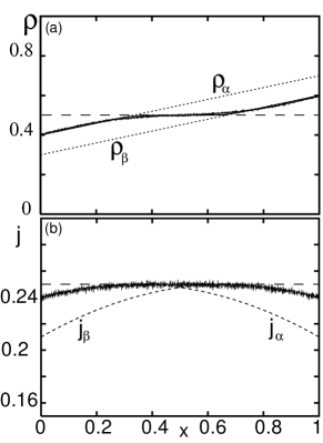
Figure 5: Average density $\rho(x)$ (a) and current $j(x)$ (b) for parameters $\alpha=0.4$, $\beta=0.4$, $\Omega=0.3$ and $K=1$. In this parameter range one observes a 3-phase coexistence: a maximal current phase is intervening between a low and high density phase. The profiles are computed analytically in the inviscid limit (dashed lines) and numerically for $\varepsilon=10^{-3}$ within a mean-field approximation (solid smooth line), and from Monte-Carlo simulations (solid wiggly line). Note that, within the resolution of the figures, the Monte-Carlo results and the numerical mean-field results can not be distinguished. The analytic density profile is shown for the solutions respecting the left and right boundaries conditions, $\rho_{\alpha}$ and $\rho_{\beta}$; we also show the Langmuir isotherm $\rho_{l}=1/2$.

(ii) For $x_{\alpha}=x_{\beta}$ the width of the intermediate maximal current phase vanishes and the solution becomes a simple linear profile, continuously matching the densities of the LD and HD phase.

(iii) Upon further increasing $x_{\alpha}$ over $x_{\beta}$, the intervening maximal current phase is lost and it is no longer possible to continuously concatenate the linear density profiles of the low and high density phase. There is necessarily a density discontinuity, located at a point $x_{w}$ where the currents corresponding to the right and left solutions match, $j_{\alpha}(x_{w})=j_{\beta}(x_{w})$. The position of the ensuing domain wall may be in or outside of the system. This leads us to further distinguish between the following three subcases:

($\mbox{iii}_{1}$) If $x_{w}<0$ the density profile in the bulk is above $1/2$, i.e. in a HD phase. The profile is entirely described by the solution $\rho_{\beta}(x)$ up to a boundary layer at the left end. One observes that the boundary layer corresponds to a discontinuity in the current. The bulk current $j_{\beta}(x\to 0^{+})$ does in general not match the incoming particle flux $\alpha(1-\alpha)$ at the left boundary (see Fig. 6).

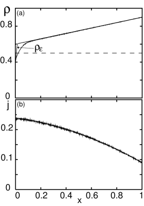
Figure 6: Average density $\rho(x)$ (a) and current $j(x)$ (b) for parameters $\alpha=0.4$, $\beta=0.1$, $\Omega=0.3$ and $K=1$. We use the same legend as in Fig. 5. The bulk profile is almost completely described by the solution $\rho_{\beta}$ matching only the right boundary condition. At the left end, the bulk density does not match the boundary condition. As a result, a boundary layer appears. Only there does one find a noticeable difference between the profiles of the Monte-Carlo simulation, the numerical computation at finite $\varepsilon$ and the analytic profile for vanishing $\varepsilon$.

($\mbox{iii}_{2}$) For $0<x_{w}<1$ the domain wall is within the system boundaries. Then the density profile connects a LD profile to a HD profile via a domain wall at position $x_{w}=(\Omega-\alpha+\beta)/2\Omega$ . The density profile is given by:

$$\rho(x)=\left\{\begin{array}[]{lcr}\Omega x+\alpha&\text{for}&0\leq x\leq x_{w}\,,\\ \Omega(x-1)+1-\beta&\text{for}&x_{w}\leq x\leq 1\,.\end{array}\right.$$ (16)

Here we can already illustrate an important feature of our model. As one can infer from Fig. 7, the current forms a cusp at the position of the domain wall, with $j_{\alpha}(x)$ and $j_{\beta}(x)$ being monotonically increasing and decreasing functions of $x$, respectively.

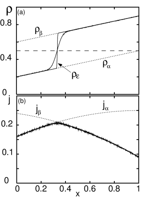
Figure 7: Average density $\rho(x)$ (a) and current $j(x)$ (b) for parameters $\alpha=0.2$, $\beta=0.1$, $\Omega=0.3$ and $K=1$. We use the same legend as in Fig. 5. Only in proximity to the domain wall the results from the mean-field approximation show deviations from the density profile obtained by Monte-Carlo simulation.

This follows directly from the continuum equation, Eq. (10), and the density dependence of the source term ${\cal F}_{A}-{\cal F}_{D}=2\Omega(1/2-\rho)$, which is positive or negative depending on whether the density is smaller or larger than $1/2$. Hence, the domain wall is located at a maximum of the current. In addition, the strict monotonicity of the current also implies that the domain wall is localized. A displacement of the domain wall to the right of $x_{w}$ would result in a current $j_{\alpha}>j_{\beta}$. This in turn would increase the influx of particles at the left boundary, which will drive the domain wall back to its original position $x_{w}$ .

($\mbox{iii}_{3}$) The solution for $x_{w}>1$ can be inferred by particle-hole symmetry from case ($\mbox{iii}_{1}$). The low density profile is given by the solution $\rho_{\alpha}(x)$ up to a boundary layer at the right end.

Lower right quadrant: $\alpha>1/2$, $\beta<1/2$.

Here the density at both left and right boundaries is larger than $\rho_{l}=1/2$. Two different scenarios are possible. In the first scenario, the slope $\Omega$ of the density profile $\rho_{\beta}(x)$ (matching the density at the right boundary) is so small that $\rho_{\beta}(x)$ is always larger than $\rho_{l}=1/2$; this requires $\Omega<1/2-\beta$. Then, the bulk of the system is in the HD phase with a boundary layer on the left. This scenario is identical to the previous case ($\mbox{iii}_{1}$), such that there is no qualitative change in the bulk upon crossing the line $\alpha=1/2$. In other words, there is no phase boundary and the system remains in the HD phase. In the second scenario, the slope $\Omega>1/2-\beta$ such that we have a phase boundary between a high density and a maximal current phase. This solution can also be viewed as a limit of the 3-phase coexistence region, where for $\alpha\to 1/2^{-}$ the phase boundary $x_{\alpha}$ leaves the system through the left end and a boundary layer is created replacing the LD region (see Figs. 8(a,b)).

Figure 8: (a)-(b) Average density $\rho(x)$ and current $j(x)$ for $\alpha=0.8$, $\beta=0.35$, $\Omega=0.3$ and $K=1$. We use the same legend as in Fig. 5. Except for the left boundary layer, in fig. (a) the analytic solution is described by the Langmuir density $\rho_{l}=1/2$ and the density $\rho_{\beta}$ matching the right boundary condition. (c)-(d) Average density $\rho(x)$ and current $j(x)$ for $\alpha=0.35$, $\beta=0.8$ and the same $\Omega$ and $K$ as before. Note that the curves map to those of (a)-(b) by particle-hole symmetry.

Upper left quadrant: $\alpha<1/2$, $\beta>1/2$.

This region in parameter space is obtained using particle-hole symmetry from the results for the lower right quadrant in the preceding paragraph (see Figs. 8(c,d)).

Upper right quadrant: $\alpha,\beta>1/2$.

Here two boundary layers are formed, and the bulk of the system is characterized by a constant density equal to $1/2$ (see Fig. 9). This corresponds to the maximal current phase, which remains unchanged as compared to the TASEP without particle on- and off-kinetics. Note again that due to $K=1$ the density with maximal current coincides with the Langmuir isotherm $\rho_{l}=1/2$.

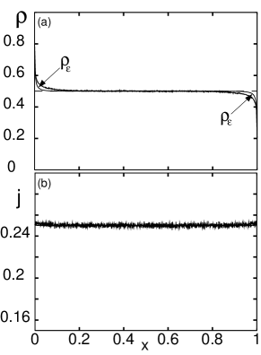
Figure 9: Average density $\rho(x)$ (a) and current $j(x)$ (b) for parameters $\alpha=0.8$, $\beta=0.8$, $\Omega=0.3$ and $K=1$. We use the same legend as in Fig. 5. The bulk density profile is given by the Langmuir density $\rho_{l}=1/2$ which corresponds also to the maximal current phase. Due to fluctuations, neglected in the mean-field approximation, the current profile obtained from the simulation exceeds the value $1/4$ at each boundary.

IV.1.2 The phase diagram

The analysis of the current and density profiles allows to draw cuts of the phase diagram in the $(\alpha,\beta)$–plane for fixed values of $\Omega$. Note that the particle-hole symmetry renders all diagrams symmetric with respect to the diagonal $\alpha=\beta$. Depending on the kinetic rate $\Omega$ one can distinguish three topologies. Topologies of the phase diagrams change at critical values $\Omega=1/2$ and $\Omega=1$; see Fig. 10.

Figure 10: Cut of the phase diagram on the $(\alpha,\beta)$–plane in the mean-field approximation for $K=1$ and different values of $\Omega$: (a) $\Omega=0.3$, (b) $\Omega=0.5$, (c) $\Omega=1.0$. The cases (a)-(c) correspond to the three different topologies of phase diagrams discussed in the main text. All lines represent continuous transitions between different regions in the $(\alpha,\beta,K=1,\Omega_{D}=\text{const.})$ cut of the $4$-dimensional parameter space. The line parallel to the anti-diagonal is defined through the relation $\alpha+\beta+\Omega=1$. It represents the border line where the points $x_{\alpha}$ and $x_{\beta}$ (i.e. the points where the left and right solutions $\rho_{\alpha}$ and $\rho_{\beta}$ meet the Langmuir isotherm $\rho_{l}=1/2$) coincide, $x_{\alpha}=x_{\beta}$. The phase boundaries of the LD-HD coexistence phase, $x_{w}=0$ and $x_{w}=1$, correspond to regions in which the domain wall is located at one of the system boundaries. These lines were computed by using the matching conditions for the currents: $j_{\alpha}(1)=\beta(1-\beta)$ and $j_{\beta}(0)=\alpha(1-\alpha)$. In figure (a), we also emphasize the presence of the boundary layers at the left or the right end of the system. These are indicated with the letters ”l” and ”r”, respectively. Such boundary layers remain present in the same regions as in figure (a) also for increasing $\Omega$.

For $0<\Omega<1/2$, Fig. 10(a), the phase diagram consists of seven phases. A 3-phase coexistence region LD-MC-HD at the center is surrounded by three 2-phase coexistence regions LD-HD, MC-HD and LD-MC. Pure LD, HD and MC phases are contiguous to the 2-phase regions. All lines between different regions represent continuous changes in the average density $\rho$. The 3-phase coexistence region, and two of the 2-phase coexistence regions (LD-MC and MC-HD) are characterized by continuous density profiles. This is mainly due to the maximal current phase with density $\rho_{l}(x)=1/2$. Acting as a ”buffer”, this phase intervenes between the LD and HD phase or connects the LD and HD phases with the right and left boundary, respectively. Discontinuities only appear as current and density discontinuities (boundary layers) at the system boundaries. This has to be contrasted with the density profile in the coexistence region between the LD and HD phase. Here, a density discontinuity in the bulk (domain wall), separating both phases, is formed.

It is also interesting to consider the limit $\Omega\rightarrow 0$, as one expects to recover the TASEP scenario. Indeed, using the previous results, it is easy to show that for decreasing $\Omega$, the width of the 2-phase regions, as well as that of the 3-phase region, shrinks to zero. The resulting diagram reproduces the well known topology of the pure TASEP in the mean-field approximation Derrida et al. (1992).

Upon increasing $\Omega$ up to the value $1/2$, we find the first topology change in the phase diagram. The HD and LD phases gradually disappear, leaving only the 2-phase or 3-phase coexistence regions at $\Omega=1/2$, see Fig. 10(b). If $\Omega$ becomes larger than $1$, the LD-HD coexistence region disappears; see Fig. 10(c).

The Langmuir kinetics is approached for $\Omega\to\infty$. Although the topology of the phase diagram does not change anymore, the phases become almost indistinguishable for large kinetic rates. Here the Langmuir isotherm $\rho_{l}=1/2$ occupies most of the bulk, whereas the LD and HD regions are confined to a vicinity of the boundaries.

IV.2 The generic case: $K>1$

Though simpler to analyze, the previous case $K=1$ is somewhat artificial as it requires a fine-tuning of the on- and off-rates. Generally, one would expect $K\neq 1$. Due to particle-hole symmetry we can restrict ourselves to $K>1$. The analysis becomes significantly more complex since the continuum equation for the density, Eq. (11), no longer factorizes into a simple form as for $K=1$.

IV.2.1 The density and current profiles

To proceed, it is convenient to introduce a rescaled density of the form

$$\sigma(x)=\frac{K+1}{K-1}\left[2\rho(x)-1\right]-1\,,$$ (17)

where $\sigma=0$ corresponds to the Langmuir isotherm $\rho_{l}=K/(K+1)$. Since the density $\rho(x)$ is bound within the interval $[0,1]$, the rescaled density $\sigma(x)$ can assume values within the interval $[-2K/(K-1),2/(K-1)]$. Then the continuum equation Eq. (11) simplifies to

$$\partial_{x}\sigma(x)+\partial_{x}\ln|\sigma(x)|=\Omega_{D}\frac{(K+1)^{2}}{K-1}\,.$$ (18)

Direct integrations yield

$$|\sigma(x)|\exp(\sigma(x))=Y(x)\,,$$ (19)

where the function $Y(x)$ is

$$Y(x)=|\sigma(x_{0})|\exp\left\{\Omega_{D}\frac{(K+1)^{2}}{K-1}(x-x_{0})+\sigma(x_{0})\right\}\,,$$ (20)

and $\sigma(x_{0})$ is the value of the reduced density at the reference point $x_{0}$. In particular, the ones that match the boundary condition on the left or right end of the system are written

$$Y_{\alpha}(x) = |\sigma(0)|\exp\left\{\Omega_{D}\frac{(K+1)^{2}}{K-1}x+\sigma(0)\right\}$$ (21)

$$Y_{\beta}(x) = \left|\sigma(1)\right|\exp\left\{\Omega_{D}\frac{(K+1)^{2}}{K-1}(x-1)+\sigma(1)\right\}\,,$$

where the boundary values $\sigma(0)$ and $\sigma(1)$ can be written in terms of $\alpha$ and $\beta$ using Eq. (17) and the boundary conditions $\rho(0)=\alpha$ and $\rho(1)=1-\beta$.

Equations of the form of Eq. (19) appear in various contexts such as enzymology, population growth processes and hydrodynamics (see e.g. Ref. Corless et al. (1996)). They are known to have an explicit solution written in terms of a special function called $W$-function Corless et al. (1996):

$$\sigma(x) = W\left(Y(x)\right)\,,\qquad\sigma(x)>0$$

$$\sigma(x) = W\left(-Y(x)\right)\,,\quad\;\sigma(x)<0\,.$$ (22)

The Lambert $W$-function (see Fig. 11) is a multi-valued function with two real branches, which we refer to as $W_{0}(\xi)$ and $W_{-1}(\xi)$. The branches merge at $\xi=-1/e$, where the Lambert $W$-function takes the value $-1$. The first branch, $W_{0}(\xi)$, is defined for $\xi\geq-1/e$ ; it diverges at infinity sub-logarithmically. The second branch, $W_{-1}(\xi)$, is always negative and defined in the domain $-1/e\leq\xi\leq 0$. In the vicinity of the point $\xi=-1/e$ the function $W(\xi)$ behaves like a square root of $\xi$ since one gets $\partial_{\xi}W=W/[(1+W)\xi]$ by the definition of the Lambert $W$-function, $W(\xi)\exp(W(\xi))=\xi$.

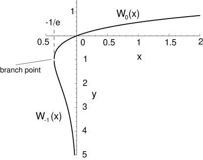
Figure 11: The real branches $W_{0}(\xi)$ and $W_{-1}(\xi)$ of the Lambert $W$-function.

Using these properties of the Lambert $W$-function, the branch of $W$ is selected according to the value of the rescaled density $\sigma$. For $\sigma\in[-2K/(K-1),-1]$ the relevant solution is $W_{-1}(-Y)$, while for $\sigma\in[-1,0]$ one obtains $W_{0}(-Y)$. Finally, in the interval $\sigma\in[0,2/(K-1)]$ one finds $W_{0}(Y)$.

The solutions are matched to the boundary conditions at the left and right ends according to the entry or exit rates. The left and right solutions, $\rho_{\alpha}(x)$ and $\rho_{\beta}(x)$, are then computed from the expressions in Eqs. (23) upon using the coordinate transformation given by Eq. (17).

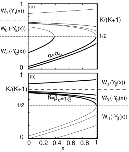
Figure 12: Mathematical solutions for (a) the left density $\rho_{\alpha}(x)$ and (b) the right density $\rho_{\beta}(x)$ for $K=3$, $\Omega_{D}=0.1$ and different values of the entry and exit rate $\alpha$ and $\beta$. The solutions which approach the Langmuir isotherm are those for $\alpha,\,\beta\leq 1/2$ (thick lines). The solutions where the branching point coincides with the right boundary are indicated by $\alpha_{c}=0.038532...$ and $\beta_{c}=1/2$.

Fig. 12 provides a graphical representation of the possible set of solutions of the first order differential equation, Eq. (18). In order to decide which one of them are actually physically realized, one needs to go back to the full equation, either in its discrete form Eq. (7a) or its continuous version Eq. (9). Analogous to the TASEP a solution matching the density prescribed by the left boundary condition is stable only if $\alpha<1/2$ . Such solutions are shown as thick lines in Fig. 12(a). They are monotonically increasing towards the Langmuir isotherm $\rho_{l}=K/(K+1)>1/2$. This can be understood as a consequence of the accumulation of particles from the bulk reservoir via the Langmuir kinetics with increasing distance from the left boundary. One might now expect that the density will finally approach the Langmuir isotherm. But, this is not the case. Instead, we find that the density $\rho_{\alpha}(x)$ never increases beyond $1/2$, where the current reaches its largest possible value $j_{\text{max}}=1/4$. Mathematically, this is a direct consequence of the analytic properties of the Lambert $W$-function, which has a branching point at a density $1/2$; see Fig. 12(a). With decreasing $\alpha$ the site where $\rho_{\alpha}(x)$ meets the density $1/2$ moves to the right. At a critical value of the entry rate, $\alpha_{c}(\Omega_{D},K)$, the branching point of the left solution $\rho_{\alpha}$ touches the right boundary.

Similarly to the discussion in the previous paragraph, solutions matching the right boundary condition are stable only if $\beta\leq 1/2$. The corresponding density profiles, shown as thick lines in Fig. 12(b), are always in a high density regime, i.e. $\rho_{\beta}(x)\geq 1/2$. If the density at the right boundary matches the Langmuir isotherm, the right solution is flat $\rho_{\beta}(x)=\rho_{l}$. Otherwise, the source terms do not cancel, leading to a net detachment/attachment flux such that the right density profiles decay monotonically towards the Langmuir isotherm as one moves from the right boundary to the bulk. As a consequence, the right density $\rho_{\beta}(x)$ never crosses the Langmuir isotherm. The density profile for $\beta=1/2$ is an extremal solution exhibiting the lowest possible density ($\rho=1/2$) and highest current ($j=1/4$) at the right end, which then also coincides with the branching point of the Lambert $W$-function.

In conclusion, for the left rescaled solution $\sigma_{\alpha}(x)$, an entry rate $0\leq\alpha\leq 1/2$ implies $-2K/(K-1)\leq\sigma\leq-1$. Hence we have according to the previous analysis:

$$\sigma_{\alpha}(x)=W_{-1}(-Y_{\alpha}(x))<0\,.$$ (23a)

For the right rescaled solution $$\sigma_{\beta}(x)$$, one finds correspondingly

$$\sigma_{\beta}(x)=\left\{\begin{array}[]{lll}W_{0}(Y_{\beta}(x))>0&,&0\leq\beta<1-\rho_{l}\\ &&\\ 0&,&\beta=1-\rho_{l}\\ &&\\ W_{0}(-Y_{\beta}(x))<0&,&1-\rho_{l}<\beta\leq 1/2\,,\end{array}\right.$$ (23b)

where $\rho_{l}=K/(K+1)$ is the constant density of the Langmuir isotherm. After the coordinate change (17), the general solution of the continuum mean-field equation at $\varepsilon\rightarrow 0^{+}$, Eq. (11), is obtained by matching left and right solutions $\rho_{\alpha}$ and $\rho_{\beta}$. The remaining task is now to identify the different scenarios where domain walls and boundary layers appear. Such analytic results are confirmed by the numerical computation at finite $\varepsilon$.

Lower left quadrant: $\alpha,\beta\leq 1/2$.

This is the only case where there are solutions that approach the Langmuir isotherm in the bulk and match both boundary conditions. The full density profile is obtained by finding the position $x_{w}$ where the left and right currents coincide, i.e. $\rho_{\alpha}(x_{w})=1-\rho_{\beta}(x_{w})$. One has to consider three cases: (i) $0<x_{w}<1$, (ii) $x_{w}<0$, and (iii) $x_{w}>1$.

In case (i), a domain wall is formed separating a region of low density on the left with a region of high density on the right. Depending on whether $1-\beta$ is above or below $\rho_{l}$, different profiles are observed, see Figs. (13)(a),(c). In the case $\beta=1-\rho_{l}$, one obtains a flat profile of $\rho_{\beta}$ matching the value of the Langmuir isotherm $\rho_{l}$. We note again that the left and right solutions approach the Langmuir isotherm in the bulk. In analogy with the case $K=1$, the domain wall is stabilized by the current profiles controlled by the boundary conditions.

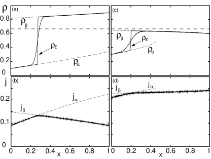
Figure 13: Average density $\rho(x)$ (a)-(c) and corresponding current $j(x)$ (b)-(d) for $\alpha,\,\beta\leq\frac{1}{2}$ in a parameter regime showing phase separation. We have chosen $\Omega_{D}=0.1$, $K=2$ and (a)-(b) $\alpha=0.1,\,\beta=0.1$ or (c)-(d) $\alpha=0.3,\,\beta=0.4$. Solid lines correspond to the numerical solution of the mean-field theory with $\varepsilon=10^{-3}$. Monte-Carlo simulations are shown as solid wiggly line. The flat dashed line represents the Langmuir isotherm, $\rho_{l}=K/(K+1)$. The other dashed lines represent the analytic solutions given by the branches of the Lambert $W$-functions matching the boundary conditions on the right and left end, respectively. For both cases (a) and (c), the solution matching the left boundary condition $\rho_{\alpha}$ is given by the branch of the Lambert $W$-function $W_{-1}(-Y_{\alpha})$. For the solution matching the right boundary condition, $\rho_{\beta}$, one has to consider the branch $W_{0}$. For (a) the branch of $W$ has the argument $Y_{\beta}(x)$, while for (c) the argument is $-Y_{\beta}(x)$ (see as illustration also Fig. 12).

In cases (ii) and (iii), one of the two phases is confined to the boundary. Explicitly, for (ii) the bulk is characterized by a HD with a boundary layer at the left end, see Fig. 14(a).

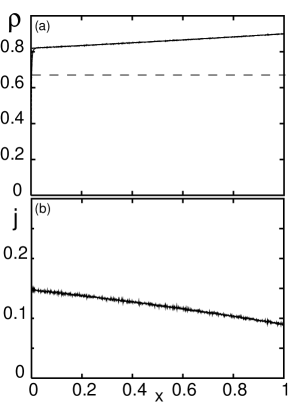
Figure 14: Average density $\rho(x)$ (a) and current $j(x)$ (b) for $\alpha=0.3$, $\beta=0.1$, $\Omega_{D}=0.1$ and $K=2$. We use the same legend as in Fig. 13. Except the left boundary layer, the bulk density profile is given by the Lambert $W$-function, $\rho_{\beta}=W_{0}(Y_{\beta}(x))$.

Correspondingly, for (iii) the solution exhibits a LD bulk phase accompanied by a boundary layer on the right end side of the system, see Fig. 15(a).

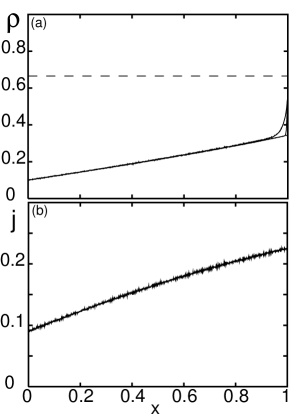
Figure 15: Average density $\rho(x)$ (a) and current $j(x)$ (b) for $\alpha=0.1$, $\beta=0.4$, $\Omega_{D}=0.1$ and $K=2$. We use the same legend as in Fig. 13. Except the right boundary layer, the bulk density profile is given by the Lambert $W$-function, $\rho_{\alpha}=W_{-1}(Y_{\alpha}(x))$.

The upper left quadrant, $\alpha<1/2$, $\beta>1/2$.

As discussed above, for $\beta>1/2$ the solutions of the first order differential equation, Eq. (11), matching the right boundary condition are physically unstable. Instead, the actual density profile at the right boundary approaches the extremal solution $W_{0}(-Y_{\beta=1/2})$ of the first order differential equation. The density difference to the boundary value is bridged by a boundary layer, which vanishes in the limit $\varepsilon\to 0^{+}$.

For the discussion of the density profiles in the upper left quadrant we can simply parallel the arguments used for the lower left quadrant, once the right solution has been substituted with the extremal one. Depending on the matching of the current, one finds again three cases, a LD phase, a 2-phase LD-HD coexistence and a HD phase. We conclude that the phases of the lower left quadrant extend to $\beta>1/2$ with phase boundaries which are independent of the exit rate $\beta$, i.e. parallel to the $\beta$ axis. The HD phase for $\beta>1/2$ has some interesting features which are genuinely distinct from the HD phase for $\beta<1/2$. The density profile in the bulk is independent of the entrance and exit rates, $\alpha$ and $\beta$, at the left and right boundaries; it is given by the extremal solution $W_{0}(-Y_{\beta=1/2})$. The density approaches $\rho(L)=1/2$ and hence the current the maximal possible value $j_{\text{max}}=1/4$ at the right boundary. These features are reminiscent of the maximal current phase for the TASEP. The only difference seems to be that here current and density are spatially varying along the system while they are constant for the TASEP. The essential characteristic in both cases is that the behavior of the system is determined by the bulk and not the boundaries. One is reminded of similar behavior of the Meissner phase in superconducting materials. In the ensuing phase diagram we will hence indicate this regime as the “Meissner” (M) phase to distinguish it from the HD phase with boundary dominated density profiles . Note also that the parameter range for the M phase is broadened as compared to the maximal current phase of the TASEP.

The remaining quadrants, $\alpha>1/2$.

At $\alpha=1/2$, the system is already in the high density phase where the bulk profile does not match the entry rate. Increasing $\alpha$ beyond the value $1/2$, therefore merely affects the boundary layer at the left end. The density profile is given by the right solution $\rho_{\beta}$ for $\beta<1/2$ or the extremal one for $\beta\geq 1/2$ as before; for an illustration compare Fig. 16. For $\beta\geq 1/2$ the same conclusion apply as in the preceding paragraph, resulting in a “Meissner” phase for the upper right quadrant.

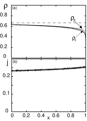
Figure 16: Average density $\rho(x)$ (a) and current $j(x)$ (b) for $\Omega_{D}=0.1$, $K=2$, $\alpha=0.75$ and $\beta=0.75$. We use the same legend as in Fig. 13. Except for the left and right boundary layers, the bulk profile obtained from the analytic mean-field result is given by the branch $\rho_{\beta}(x)=W_{0}(-Y_{\beta}(x))$ of the Lambert $W$-function computed for $\beta=1/2$.

Let us conclude this subsection with some additional comments on boundary layers. Boundary layers arise from a mismatch between the bulk profile and the boundary conditions. They can bend either upwards or downwards depending on whether the left or right boundary rates are above or below the values of the bulk solution at the ends. For example, in the right lower quadrant of the HD phase, a change from a depletion to an accumulation layer at the left end of the system occurs at $\alpha=\rho_{\beta}(0)$ for $\beta<1/2$.

IV.2.2 The phase diagram

We discuss the topology of the phase diagram with respect to cuts in the $(\alpha,\beta)$–plane for different values of $K$ and $\Omega_{D}$. We first consider the situation in which $\Omega_{D}$ is fixed and $K$ increases, starting from values slightly larger than unity. Figure 17(a) shows the phase diagram for $K=1.1$. A low density (LD) phase occupies the upper left of the plane, while a high density (HD) and a Meissner (M) phase are located on the right. In between there is a 2-phase coexistence region (LD-HD). In the coexistence phase a domain wall is localized at the point $x_{w}$ in the bulk. The boundaries of the coexistence region in the phase diagram are determined by those parameters where the domain wall hits either the entrance, i.e. $x_{w}=0$, or the exit of the system, $x_{w}=1$. For $\beta>1/2$, the density profile only develops a boundary layer at the right end, but remains unchanged in the bulk. Since the domain wall position becomes independent of $\beta$, the boundaries of the 2-phase coexistence region become parallel to the axis $\alpha=0$. It is important to remark that from the analytic results the left solution $\rho_{\alpha}$ is strictly smaller than $1/2$, except for the special point $C$ in the phase diagram where $\rho_{\alpha}(1)=\beta=1/2$. We shall see in Section V.2 that in the vicinity of this point the domain wall exhibits critical properties.

Upon increasing $K$, the LD phase progressively shrinks to a region close to the $\beta$-axis, while the size of the two other phases increases; see Figs. 17(b) and 17(c). A change of topology occurs when the LD phase collapses on this axis which happens upon passing a critical value of $K$. This critical value depends on $\Omega_{D}$ and can be computed using the expressions in Eqs. (13) and (23). A further increase of $K$ results in a decrease of the extension of the LD-HD region in the phase diagram, see Figs. 17. Eventually, for very large $K$ the average bulk density in the HD and M regions approaches saturation $\rho_{bulk}=1$.

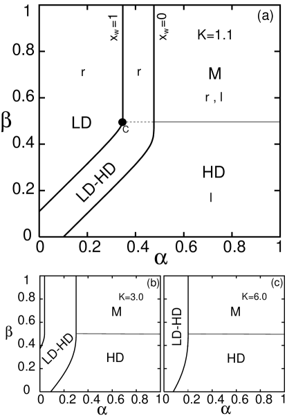
Figure 17: Cuts of the phase diagrams on the $(\alpha,\,\beta)$–plane obtained by the exact solution of the stationary mean-field equation (11) in the inviscid limit $\varepsilon=0$ for $\Omega_{D}=0.1$ and (a) $K=1.1$, (b) $K=3.0$, (c) $K=6.0$. The two lines, corresponding to regions in which the domain wall is located at $x_{w}=0$ and $x_{w}=1$, are obtained by using the matching conditions for the currents: $j_{\alpha}(1)=\beta(1-\beta)$ and $j_{\beta}(0)=\alpha(1-\alpha)$. In figure (a), we emphasize several features. With the letters ”l” and ”r” we indicate the presence of boundary layers in the average density profile, forming at the left or the right end of the system, respectively. In the lower left quadrant, the left and right boundary layers form whenever the domain wall exits the system on the left and right end side. At the phase boundary between the HD and M phases, for $\beta=1/2$, a boundary layer forms at the right end. Note that also in the M phase $\rho_{bulk}>1/2$. The presence of boundary layers in the different phases of the $(\alpha,\,\beta)$–plane is conserved upon variation of the binding constant $K$. The filled black circle represents the critical point $C$ where the domain wall exhibits critical behavior; see Sect. V.2. This critical point exits the plane for large values of $K$, accompanied with a topological change of the phase diagram.

Similarly, increasing $\Omega_{D}$ at fixed $K$, the same topology change occurs, as described above; see Fig. 18. However, we note the different limiting behaviors for $\Omega_{D}\to 0^{+}$ and $\Omega_{D}\to\infty$. In the first case, we are considering the limit of the model to the TASEP for a given binding constant $K$ (although $K\neq 1$). The 2-phase coexistence region LD-HD shrinks continuously to the line $\alpha=\beta$. In the same limit, in the upper right quadrant, $\alpha,\beta>1/2$, the M phase approaches continuously the MC phase of the TASEP. For a very large detachment rate $\Omega_{D}$, the right boundary of the LD-HD coexistence phase approaches a straight line at finite entry rate $\alpha$ that can be computed from the analytic solution as equal to $1-\rho_{l}$. In the same limit, the average density in the bulk reaches asymptotically the value $\rho_{bulk}=\rho_{l}$ of the Langmuir isotherm.

Figure 18: Cuts of the phase diagrams as in Fig. 17 for $K=3$ and (a) $\Omega_{D}=0.01$, (b) $\Omega_{D}=0.05$, (c) $\Omega_{D}=0.2$. The white circle corresponds to a nodal point of the system ${\cal N}$ defined by the condition $\alpha=\beta=1-\rho_{l}=1/(K+1)$. Every line $x_{w}=0$ crosses this point for an increasing $\Omega_{D}$.

Eventually, one observes that all phase boundaries between the LD-HD coexistence and the HD phase, i.e. where the domain is pinned at $x_{w}=0$, intersect at the same point ${\cal N}$ for any value of the detachment rate $\Omega_{D}$. This nodal point ${\cal N}$ can be evaluated as $\alpha=\beta=1-\rho_{l}=1/(K+1)$. At this point, indeed, the average density $\rho$ is given by the flat profile of the Langmuir isotherm $\rho_{l}=K/(K+1)$ which is obviously independent of $\Omega_{D}$. As a result, the domain wall does not move from $x_{w}=0$ for any value of the detachment rate $\Omega_{D}$. Interestingly, one remarks that both points $C$ and ${\cal N}$ approach continuously the triple point of the TASEP $\alpha=\beta=1/2$ in the simultaneous limit $\Omega_{D}\to 0^{+}$ and $K\to 1^{+}$.

V Domain wall properties

The knowledge of the analytic solution in the mean-field approximation allows for a detailed study of the behavior of the domain wall height and position upon a change of the system parameters. While the results for the symmetric case $K=1$ are more or less trivial, novel properties emerge for $K>1$. In this Section, we shall start from the description of the domain wall behavior on the $(\alpha,\beta)$–plane of the phase diagram along trajectories of constant entry or exit rates, respectively.

V.1 Position and amplitude of the domain wall on the $(\alpha,\beta)$–plane

Figures 19(a,b) show the dependence of the domain wall position, $x_{w}$, and height, $\Delta_{w}$, on the entry rate $\alpha$ along lines of constant exit rate $\beta$. As can be inferred from the structure of the phase diagram presented in the preceding Section, for a small enough exit rate $\beta$, a domain wall can form in the bulk with a finite amplitude even for a vanishing entry rate, $\alpha=0$. For larger $\beta$, one observes that the domain wall builds up with a finite height on the right boundary only above some specific value of $\alpha$. If one regards the domain wall height as a kind of order parameter for the coexistence phase such a behavior can be termed a first order transition. This has to be contrasted with the case $\beta=0.5$, where the domain wall enters the system at $x_{w}=1$ with infinitesimal height at a critical entry rate $\alpha=\alpha_{c}$. In the same terminology this would then be a second order transition. Indeed, as we are going to discuss in the next subsection, the domain wall exhibits critical properties at this point. In the phase diagram (Fig. 17(a)) the corresponding critical point is indicated as $C$.

In all cases, upon increasing $\alpha$ and hence the influx of particles, the domain wall changes its position continuously from the right to the left end of the system. Then, at some value $\alpha$ which depends on $\beta$, the domain wall leaves the system with a finite amplitude $\Delta_{w}$.

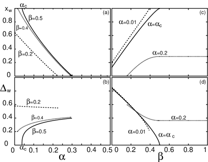
Figure 19: (a)-(b) Domain wall position $x_{w}$ and height $\Delta_{w}$ as a function of the entrance $\alpha$ for different values of the exit rate $\beta$ at $\Omega_{D}=0.1$ and $K=3$. At the critical point $\alpha=\alpha_{c}$ and $\beta=1/2$ a domain wall forms at the right end of the system with an infinitesimal height $\Delta_{w}$. The value of the ”critical” entry rate is $\alpha_{c}=0.038532...$ and can be written explicitly by using the analytic solution in the mean-field approximation, see Eq. (25). (c)-(d) Domain wall position $x_{w}$ and height $\Delta_{w}$ as a function of the exit rate $\beta$ for different values of the entrance rate $\alpha$ at $\Omega_{D}=0.1$ and $K=3$. For $\alpha=\alpha_{c}$ and $\beta=1/2$ a domain wall forms at the right end of the system with an infinitesimal height $\Delta_{w}$. For exit rates $\beta>1/2$, both domain wall position $x_{w}$ and height $\Delta_{w}$ become independent of $\beta$. Changes in the exit rate only affect the size and shape of the boundary layer on the right end, but not the bulk density profile.

Similar behaviors of the position and height of the domain wall is found as a function of $\beta$ for fixed values of $\alpha$; see Fig. 19(c,d). Here one finds that, upon increasing $\beta$ and hence reducing the out-flux of particles the domain wall position $x_{w}$ moves continuously from the left to the right boundary . For small $\alpha$, a domain wall is formed at a finite position $x_{w}$ and $\beta=0$. For larger entry rates, the domain wall forms at $x_{w}=0$ with a finite amplitude only for finite values of the exit rate $\beta$. As before, the amplitude of the domain wall $\Delta_{w}$ vanishes only for the critical value $\alpha=\alpha_{c}$ at $\beta=1/2$. Indeed, when $\alpha>\alpha_{c}$ and $\beta>1/2$, one notes that the domain wall position $x_{w}$ remains constant upon changing $\beta$. As we have explained above, this corresponds to the situation where the bulk profile is unaffected by a change in the exit rate (M phase). Only the magnitude of the boundary layer changes with increasing $\beta$.

V.2 Critical properties of the domain wall

In this Section, we discuss the domain wall properties close to the special point $C$ where the domain wall forms with infinitesimal height. The analysis will make use of the analytic solution in the mean-field approximation. We show that the domain wall emerges as a consequence of a bifurcation phenomenon, and calculate the resulting non-analytic behavior of its height and position.

At the point $C$, the analytic solution of the mean-field equations is described by a low density profile $\rho(x)=\rho_{\alpha}(x)$ that not only matches the boundary conditions at the left but also the one at the right end; see Fig. 20.

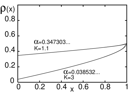
Figure 20: Average density profiles computed analytically in the inviscid limit expressed in terms of Lambert $W$-function (dashed lines) and numerically for $\varepsilon=10^{-3}$ within a mean-field approximation (solid smooth line). Parameters are: $\alpha=\alpha_{c}$ (see Eq. (25) for the analytic expression), $\beta=0.5$, $\Omega_{D}=0.1$ and different values of $K$. The profile is entirely given by the left solution $\rho_{\alpha}$ for the value of the entry rate $\alpha_{c}$, defined by the condition $\rho_{\alpha}(x=1)=1/2$, and $\beta=1/2$. Note that in this case, $\rho_{\alpha}$ matches simultaneously the left and the right boundary conditions.

This implies that the left and right currents also match at the right end of the system. Interestingly, at this position the current $j$ is maximal . By a small change of the system parameters in the 2-phase LD-HD coexistence region the domain wall forms at the right end characterized by a small height, provided that $\beta\leq 1/2$.

Using the analytic solution (23) one can give an explicit expression of the critical point $C$ as a function of $\Omega_{D}$ and $K$. The condition that the left boundary matches the value $1/2$ at $x=1$ translates to $\sigma_{\alpha}(x=1)=-1$ or, using the properties of the Lambert $W$-function, as:

$$Y_{\alpha}(x=1)=1/e\,.$$ (24)

From the expression of the function $Y_{\alpha}$, Eq. (21), and the initial condition $\sigma(0)=(2\alpha-1)(K+1)/(K-1)-1$, one computes the value of the critical entry rate

$$\alpha_{c}\!=\!\!\frac{K}{(K+1)}+\frac{K-1}{2(K+1)}W_{-1}\!\!\left(\!\!-\exp\!\left\{\!\!-\Omega_{D}\frac{(K+1)^{2}}{(K-1)}\!-\!1\!\right\}\!\!\right)\!\!\,.$$ (25)

From the discussion of the phase diagram and the general properties of the domain wall, one already infers that $0<\alpha<1/2$ for not too large values of $\Omega_{D}$ and $K$.
The set

$$(\alpha=\alpha_{c}(K,\Omega_{D}),\,\beta=1/2,\,K,\,\Omega_{D})$$ (26)

defines a two dimensional smooth manifold in parameter space (critical manifold).

In order to study the critical properties close to this manifold we apply standard methods of bifurcation theory Arnold et al. (1999); Wiggins (1990); J. Guckenheimer et al. (1997). We consider a smooth path in the region of parameter space close to the critical manifold defined above. At some point $C$ this path will cross the critical manifold. The small quantities that describe the behavior of the domain wall close to the critical manifold are the distance from the right end side, $\delta x_{c}\equiv 1-x_{w}$, and the domain wall height, $\Delta_{w}=\rho_{\beta}(x_{w})-\rho_{\alpha}(x_{w})$. These quantities will be expressed to leading order in terms of the small deviations from the critical point $\delta\alpha=\alpha-\alpha_{c}$, $\delta\beta=\beta-1/2$, and similarly for $\delta\Omega_{D}$ and $\delta K$.

The matching condition of the left and right currents, $\rho_{\alpha}(x_{w})+\rho_{\beta}(x_{w})=1$, can be rewritten in terms of reduced densities $\sigma$ as $\sigma_{\alpha}(x_{w})+\sigma_{\beta}(x_{w})=-2$. As a consequence, the solution close to the critical point writes as $\sigma_{\alpha,\beta}(x_{w})=-1\mp\Delta\sigma$, where we have introduced the reduced domain wall height $\Delta\sigma$ as another small quantity. The relation between $\delta x$ and $\Delta\sigma$ can be obtained by expanding the equality

$$\sigma_{\beta}\exp{(\sigma_{\beta})}=-Y_{\beta}(x_{w})\,,$$ (27)

leading to

$$\delta x\sim(\Delta\sigma)^{2}\,,$$ (28)

where the prefactor can be explicitly computed and depends only on the value of the system parameters at the critical point $C$. A second relation connecting $\Delta\sigma$ to the small distances $\delta\alpha,\,\delta\beta,\,\delta K$ and $\delta\Omega_{D}$ arises from the definition of the Lambert $W$-function $|\sigma|\exp(\sigma)=Y$ by taking the ratio

$$\frac{\sigma_{\beta}}{\sigma_{\alpha}}\exp{(\sigma_{\beta}-\sigma_{\alpha})}=\frac{Y_{\beta}(x_{w})}{Y_{\alpha}(x_{w})}\,.$$ (29)

The important observation is that the right-hand side is independent of the domain wall position $x_{w}$; see Eq. (21). Expanding Eq. (29) to leading order, one obtains:

$$(\Delta\sigma)^{3}\sim\delta O=A_{\alpha}\delta\alpha+A_{\beta}(\delta\beta)^{2}+A_{K}\delta K+A_{\Omega}\delta\Omega_{D}\,,$$ (30)

where $\delta O$ is a distance along a generic path that ends on the critical manifold. We do not consider the non-generic case where the the critical manifold is approached tangentially. Then one finds power laws different from those presented below for the generic case.

As before, the coefficients $A$ can be computed explicitly and shown to depend only on the rates at the critical point $C$. Interestingly, the distance $\delta O$ does not exhibit a linear term in $\delta\beta$. This is due to the singular behavior of the density profile $\rho_{\alpha}(x)$ close to the right boundary at the critical point $C$; see Fig. 20. Combining the two expansion, one finds the following power laws:

$$\delta x\sim\delta O^{2/3} \Delta_{w}\sim\delta O^{1/3}\,.$$ (31)

The validity of these exponents is confirmed numerically in Figs. 21.

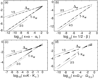
Figure 21: Double decimal logarithmic plots of the critical behavior of the domain wall height, $\Delta_{w}$, and position from the right end side, $1-x_{w}$. We obtained the plot numerically with the program Maple, release 7, using the analytic mean-field solution in the vicinity of the critical point $C$ and applying the matching condition over the left and right currents, $j_{\alpha}(x_{w})=j_{\beta}(x_{w})$. (a) As a function of $\alpha$ starting from the point $C$ on the critical manifold with coordinates $\alpha_{c}=0.038532...$, $\beta=1/2$, $\Omega_{D}=0.1$ and $K=3$. (b) As a function of $\beta$ starting from the point $C$ on the critical manifold with coordinates $\alpha=0.038532...$, $\beta_{c}=1/2$, $\Omega_{D}=0.1$ and $K=3$. (c) As a function of $K$ from the point $C$ on the critical manifold with coordinates $\alpha=0.2$, $\beta=1/2$, $\Omega_{D}=0.051443...$ and $K_{c}=3$. (d) As a function of $\Omega_{D}$ from the point $C$ on the critical manifold with coordinates $\alpha=0.2$, $\beta=1/2$, $\Omega_{D,c}=0.051443...$ and $K=3$. The value of $\Omega_{D,c}$ can be easily obtained from Eq. (21) and the initial condition $\sigma(0)$. Note the different scaling regime for the exit rate $\beta$.

We also checked that the amplitudes in the expansions (31) coincide with those obtained by the numerical data.

V.3 Further properties of the domain wall position

In this Section we discuss how the position of the domain wall $x_{w}$ moves upon changing $\Omega_{D}$ for fixed $\alpha$ and $K>1$ and a set of different values for $\beta$. In the first quadrant, $\alpha,\beta<1/2$, and for very small values of $\Omega_{D}$ the coexistence phase is confined to a narrow strip parallel to the diagonal $\alpha=\beta$; see Fig. 18(a). It extends to the quadrant $\alpha<1/2,\beta>1/2$, where boundary layers form. On the other hand, for very large $\Omega_{D}$ the coexistence phase corresponds to the region $\alpha<1-\rho_{l}$, see Sect. IV.2.2. The interesting features therefore arise in the region of $\alpha<1-\rho_{l}$ and $\beta<1/2$. We consider a path in the phase diagram with fixed $\alpha,\beta$ and $K$ and follow how it intersects the phase boundaries of the 2-phase coexistence region LD-HD as $\Omega_{D}$ is increased. From Fig. 22 one can distinguish three cases.

For $\alpha<\beta$ the system is in a LD phase for very small $\Omega_{D}$. Then, at a critical value of $\Omega_{D}$ it enters the LD-HD region where a domain wall forms at the right boundary. A further increase of $\Omega_{D}$ results in a change of the domain wall position to the left, asymptotically reaching the left boundary for very large values of the detachment rate $\Omega_{D}$.

For $\beta<\alpha$, the system is in the HD region for small $\Omega_{D}$. By increasing the detachment rate, it enters the LD-HD region. Differently from the previous case, the domain wall now forms at the left boundary, it moves to the right up to a maximal position $x_{m}$ for intermediate values of $\Omega_{D}$, and finally for large $\Omega_{D}$ it moves back to the left boundary with the same asymptotic behavior as the previous case.

For $\beta=\alpha$, the system remains in the 2-phase coexistence region LD-HD for all values of the detachment rate $\Omega_{D}$. One can prove, using the analytic solution (23), that the domain wall position stays finite even in the limit $\Omega_{D}\to 0^{+}$ and is given by

$$x_{w}=\frac{\sigma(1)(1+\sigma(0))}{2(\sigma(0)\sigma(1)-1)}\,,$$ (32)

where $\sigma(0)$ and $\sigma(1)$ are the usual boundary conditions written in terms the model parameters; see Eq. 17.

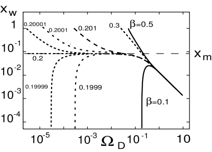
Figure 22: Domain wall position $x_{w}$ in logarithmic scale as a function of $\Omega_{D}$ at $\alpha=0.2$, $\Omega_{D}=.051443...$ and $K=3$ and different values of $\beta$. If $\beta>\alpha$ the domain wall builds up from the right boundary, while for $\beta<\alpha$ from the left boundary. For $\alpha=\beta$ the domain wall approaches the position $x_{m}$ which is independent of the decreasing detachment rate $\Omega_{D}$. At large $\Omega_{D}$ the domain wall position $x_{w}$ always moves to the left boundary as $1/\Omega_{D}$.

Interestingly, the domain wall position $x_{w}$ obtained for $\alpha=\beta$ and vanishing $\Omega_{D}$ does not reduce to the value given by the mean-field continuum approximation in a pure TASEP, i.e. $x_{w}=1/2$. In order to regain the TASEP position, the binding constant $K$ has to approach the unity. Moreover, from Eq. (32) one find that in the limit $\alpha=\beta\to 1/2^{-}$, the position $x_{m}$ is a singular function of the binding constant close to $K=1^{+}$.

The previous discussion corroborates the fact that the Langmuir Kinetics constitutes a singular perturbation of the TASEP even in the limit of small rates, yielding new features that are generated by the competition between the two dynamics.

VI Conclusions

We have presented a detailed study of a model for driven one-dimensional transport introduced recently in Ref. Parmeggiani et al. (2003), where the dynamics of the totally asymmetric simple exclusion process has been supplemented by Langmuir kinetics. This non-conservative process introduces competition between boundary and bulk dynamics suggesting a new class of models for non-equilibrium transport. The model is inspired by essential properties of intracellular transport on cytoskeletal filaments driven by processive motor proteins Alberts et al. (1994); Howard (2001). These molecular engines move unidirectionally along cytoskeletal filaments, and simultaneously are subject to a binding/unbinding kinetics between the filament and the cytoplasm. The processivity of the motors implies low rates of detachment. Attachment rates can be easily tuned by changing the concentration of motors in the cytoplasm. In particular one may obtain very low attachment rates using a low volume concentration of motors.

The non-conservative dynamics proposed introduces a non-trivial stationary state, with features qualitatively different from both the totally asymmetric simple exclusion process and Langmuir kinetics. The competing dynamics leads to an unexpected spatial modulation of the average density profile in the bulk. For extended regions in parameter space, we find that the density profile exhibits discontinuities on the scale of the system size which is characteristic for phase separation. Furthermore, the coexisting phases manifest themselves by a domain wall that, contrary to the TASEP, is localized in the bulk. In contrast to previous models Kolomeisky (1998); Mirin and Kolomeisky (2003), the localization is not induced by local defects, but arises via a collective phenomenon based on a microscopically homogeneous bulk dynamics. The resulting phase diagram is topologically distinct from the totally asymmetric exclusion process and exhibits new phases.

An analytic solution for the density profile has been derived in the context of a mean-field approximation in the continuum limit. The properties of the average density for different kinetic rates are encoded in the peculiar features of the Lambert $W$-function. In particular, the discovery of a branching point is a prerequisite to rationalizing the behavior of the solution. The analytic solution has allowed to trace and study in detail the properties of the phase diagram. We found that the cases of equal and different binding rates give rise to rather distinct topologies in the phase diagram. The limiting cases for small or large kinetic rates have been computed analytically. We have identified special points of the phase diagram which are the analogue of the ”triple point” (viz. where all three phase boundaries meet) of the totally asymmetric simple exclusion process. There, a domain wall builds up with infinitesimal height at the boundary, exhibiting critical features characterized by unusual mean-field exponents. Finally, we have discussed some limiting cases in which the properties of the totally asymmetric simple exclusion process in the mean-field approximation are recovered.

Let us give some more intuitive arguments on the domain wall formation and localization. In the limit of large system sizes, the corresponding time-dependent version of Eq. (11) which governs the dynamics of the ”coarse-grained” density $\rho$ reads

$$\partial_{t}\rho+(1-2\rho)\partial_{x}\rho={\cal F}_{A}-{\cal F}_{D}\,.$$ (33)

One can easily see that on hydrodynamic scales the source contribution on the right hand side are negligible compared to the terms related to the transport dynamics. On these scales, the local dynamics is essentially described by mass conservation just as in the totally asymmetric exclusion process. Neglecting the source contribution, one can give an implicit analytic solution of Eq. (33) by standard methods of partial differential equations Zwillinger (1997); Zachmanoglou and Thoe (1986). From such analysis, one can infer the mechanism of the formation of density discontinuities such as shocks on the hydrodynamic scale, which usually build up in finite time. An interesting feature of the domain wall is also its slope $S_{w}$  as a function of the system size $N$. In Fig. 23 we show the slope of the domain wall as obtained from Monte-Carlo simulation for growing system size $N$. We find the scaling law $S_{w}\sim N^{\eta}$ with the exponent $\eta=0.50\pm 0.05$.

Figure 23: Domain wall slope $S_{w}$ estimated from Monte Carlo simulations as a function of the system size $N$. Simulations where performed for $\alpha=0.2$, $\beta=0.6$, $K=3$ and $\Omega_{D}=0.1$.

This result is fully compatible with the scaling exponent $\eta=1/2$ computed for a pure totally asymmetric exclusion process. Note that the mean-field approximation provides a wrong exponent $\eta_{MFA}=1$. The softening of the slope compared to mean-field was recently explained in Ref.  Evans et al. (1998); Popkov et al. (1998) on the basis of domain wall fluctuations Kolomeisky et al. (1998). In this picture, the fluctuating domain wall performs a random walk just like in the totally asymmetric exclusion process. However, since on global scale there is no mass conservation due to the Langmuir kinetics, the current is space dependent and drives the domain wall to an equilibrium position corresponding to a cusp in the current profile. Such domain wall behavior can be rephrased in terms of a random walk in the presence of a confining potential Rakos et al. (2003). This picture also suggests that the exponent for the slope of the domain wall is exactly given by $\eta=1/2$.

It would be interesting to study how the case of equal rates can be obtained by a limiting procedure of the case with slightly different rates. The change of topology in the phase diagrams should be contained in the analytic solution, however one suspects from Eq. (21) that an essential singularity appears. Furthermore, one would like to see if possible variants of our model introduce new features similar to what has been done for a reference dynamics, i.e. the totally asymmetric exclusion process Schütz (2003).