Regularly alternating spin–$\frac{1}{2}$ anisotropic $XY$ chains:
The ground–state and thermodynamic properties

Abstract

Using the Jordan–Wigner transformation and continued fractions we calculate rigorously the thermodynamic quantities for the spin–$\frac{1}{2}$ transverse Ising chain with periodically varying intersite interactions and/or on–site fields. We consider in detail the properties of the chains having a period of the transverse field modulation equal to 3. The regularly alternating transverse Ising chain exhibits several quantum phase transition points, where the number of transition points for a given period of alternation strongly depends on the specific set of the Hamiltonian parameters. The critical behavior in most cases is the same as for the uniform chain. However, for certain sets of the Hamiltonian parameters the critical behavior may be changed and weak singularities in the ground–state quantities appear. Due to the regular alternation of the Hamiltonian parameters the transverse Ising chain may exhibit plateau–like steps in the zero–temperature dependence of the transverse magnetization vs. transverse field and many–peak temperature profiles of the specific heat. We compare the ground–state properties of regularly alternating transverse Ising and transverse $XX$ chains and of regularly alternating quantum and classical chains.

Making use of the corresponding unitary transformations we extend the elaborated approach to the study of thermodynamics of regularly alternating spin–$\frac{1}{2}$ anisotropic $XY$ chains without field. We use the exact expression for the ground–state energy of such a chain of period 2 to discuss how the exchange interaction anisotropy destroys the spin–Peierls dimerized phase.

I Introductory remarks

The spin–$\frac{1}{2}$ Ising chain in a transverse field (transverse Ising chain) is known as the simplest model in the quantum theory of magnetism. It can be viewed as the 1D spin–$\frac{1}{2}$ anisotropic $XY$ model in a transverse ($z$) field with extremely anisotropic exchange interaction. By means of the Jordan–Wigner transformation it can be reduced to a 1D model of noninteracting spinless fermions001 ; 002 ; 003 ; 004 . As a result the transverse Ising chain appeared to be an easy case005 and a lot of studies on that model have emerged up till now. After the properties of the basic skeleton model were understood various modifications were introduced into the model and the effects of the introduced changes were examined. For example, an analysis of the critical behavior of the chain with an aperiodic sequence of interactions was performed in Ref. 006, , an extensive real–space renormalization–group treatment of the random chain was reported in Ref. 007, , a renormalization–group study of the aperiodic chain was presented in Ref. 008, . It should be remarked, however, that the simpler case of the regularly inhomogeneous spin–$\frac{1}{2}$ transverse Ising chain (in which the exchange interactions between the nearest sites and/or the on–site transverse fields vary regularly along the chain with a finite period $p$) still contains enough not explored properties which deserve to be discussed. Moreover, the thermodynamic quantities of such a system can be derived rigorously analytically exploiting the fermionic representation and continued fractions.

The thermodynamic properties of the regularly alternating anisotropic $XY$ chain in a transverse field of period 2 were considered in Refs. 009, ; 010, (see also Ref. 011, where a model without field was investigated). The elaborated general approach for calculation of thermodynamic quantities010 becomes rather tedious if $p>2$ and the properties of chains of larger periods of alternation were not discussed. Other papers012 ; 013 are devoted to the 1D anisotropic $XY$ model on superlattices, which can be viewed as particular cases of a regularly alternating anisotropic $XY$ chain. In Ref. 012, the transfer matrix method was applied to get the excitation spectrum of the Hamiltonian, being a quadratic form of creation and annihilation Bose or Fermi operators, on a 1D superlattice. (This fermionic system is related to the 1D spin–$\frac{1}{2}$ transverse anisotropic $XY$ model on a superlattice.) In Ref. 013, a version of the approach suggested in Ref. 010, was applied to superlattices. Considering as an example the ground–state dependences of the transverse magnetization vs. transverse field and of the static transverse susceptibility vs. transverse field (which were examined numerically for an anisotropic $XY$ chain of period 4) the authors of Ref. 013, observed that these quantities behave differently than for the isotropic $XY$ model. Contrary to the case of isotropic $XY$ model, for the anisotropic $XY$ model the number of the critical fields at which the susceptibility becomes singular strongly depends on the specific values of intersite interaction parameters. The quantum critical points in the anisotropic $XY$ chains in a transverse field with periodically varying intersite interactions (having periods 2 and 3) were determined using the transfer matrix method in Ref. 014, . It was found that for periodic chains the number of quantum phase transition points may increase and its actual value depends not only on the period of modulation but also on the strengths of anisotropy and modulation of exchange interactions. Let us also mention here a paper discussing the energy gap vanishing in the dimerized (i.e., period 2) anisotropic $XY$ chain without field015 and a recent paper016 which contains such an analysis for a nonzero transverse field.

In the present paper we have obtained a number of new results for regularly alternating spin–$\frac{1}{2}$ anisotropic $XY$ chains exploiting a systematic method for the calculation of the thermodynamic quantities not used in the references cited above. This approach is based on exploiting continued fractions017 and seems to be a natural and convenient language for describing regularly alternating chains (Section II). Considering the chains of period 3 we examine the generic effects induced by regular alternation. We discuss, in particular, the effect of regular alternation on the energy gap (Sections II and III), the zero–temperature dependences of the transverse magnetization vs. transverse field and of the static transverse susceptibility vs. transverse field, and the temperature dependence of the specific heat (Section III). These rigorous analytical results completed by numerical calculations of the spin correlation functions (Section III) demonstrate the effect of the regular alternation of Hamiltonian parameters on the quantum phase transition inherent in the spin–$\frac{1}{2}$ transverse Ising chain. Although in most cases the critical behavior remains like in the uniform chain case, for certain sets of the Hamiltonian parameters weak singularities in the ground–state quantities may appear. We compare the results for the transverse Ising chains with the corresponding ones for the isotropic $XY$ chains in a transverse field (transverse $XX$ chains); moreover, we also compare the ground–state properties of the quantum and classical regularly alternating transverse Ising/$XX$ chains (Section III).

The results obtained exploiting the continued fraction approach can be used to examine the thermodynamics of the regularly alternating spin–$\frac{1}{2}$ anisotropic $XY$ chain without field since the latter model is related to a system of two spin–$\frac{1}{2}$ transverse Ising chains through certain unitary transformations. We use the exact expression for the ground–state energy of the anisotropic $XY$ chain without field of period 2 to demonstrate the effects of anisotropy of exchange interaction on the spin–Peierls dimerization (Section IV).

We end up this Section introducing notations and making some symmetry remarks. We consider $N\to\infty$ spins $\frac{1}{2}$ on a ring governed by the Hamiltonian

$$H=\sum_{n=1}^{N}\Omega_{n}s_{n}^{z}+\sum_{n=1}^{N}2I_{n}s^{x}_{n}s^{x}_{n+1}$$ (1.1)

(with $s_{N+1}^{\alpha}=s_{1}^{\alpha}$ ($I_{N}=0$) for periodic (open) boundary conditions). Here $I_{n}$ is the (Ising) exchange interaction between the nearest sites $n$ and $n+1$ and $\Omega_{n}$ is the transverse field at the site $n$. We assume that these quantities vary regularly along the chain with period $p$, i.e., the sequence of parameters in (1.1) is $\Omega_{1}I_{1}\Omega_{2}I_{2}\ldots\Omega_{p}I_{p}\Omega_{1}I_{1}\Omega_{2}I_{2}\ldots\Omega_{p}I_{p}\ldots\;$. Our goal is to examine the thermodynamic properties of the spin model (1.1).

Let us extend the “duality” transformation018 ; 003 to the inhomogeneous case (for the Ising chain in a random transverse field such a transformation was discussed in Refs. 009, ; 019, ). It can be easily proved that the partition function $Z={\mbox{Tr}}\exp\left(-\beta H\right)$ for two sequences of parameters $\ldots\Omega_{n}I_{n}\ldots$ and $\ldots I_{n-1}\Omega_{n}\ldots$ (or $\ldots I_{n}\Omega_{n+1}\ldots\;$) is the same. That means that the fields and the interactions may be interchanged as $\Omega_{n}\to I_{n-1}$ and $I_{n}\to\Omega_{n}$ (or $\Omega_{n}\to I_{n}$ and $I_{n}\to\Omega_{n+1}$) remaining the partition function unchanged. Really, performing the unitary transformation $U=\prod_{p=1}^{N-1}\exp\left({{\mbox{i}}\pi s_{p}^{x}s_{p+1}^{y}}\right)$ one finds that Eq. (1.1) transforms (with the accuracy to the end terms not important for the thermodynamics) into

$$UH{U}^{+}=\sum_{n=1}^{N}I_{n}s_{n+1}^{z}+\sum_{n=1}^{N}2\Omega_{n}s^{y}_{n}s^{y}_{n+1}$$

$$=\sum_{n=1}^{N}I_{n}s_{n}^{z}+\sum_{n=1}^{N}2\Omega_{n+1}s^{y}_{n}s^{y}_{n+1}$$ (1.2)

(to get the second equality we have renumbered the sites $n\to n-1$ which obviously does not change the thermodynamics). As a result $R^{z}UHU^{+}{R^{z}}^{+}$ with $R^{z}=\prod_{q=1}^{N}\exp\left({\mbox{i}}\frac{\pi}{2}s_{q}^{z}\right)$ (up to the end effects) is again the transverse Ising chain, however, with the exchange interaction between the nearest sites $n$ and $n+1$ being equal to $\Omega_{n}$ (or $\Omega_{n+1}$) and the transverse field at the site $n$ being equal to $I_{n-1}$ (or $I_{n}$).

We also recall that the unitary transformation $F_{m}=2s_{m}^{x}$ changes the sign of the transverse field at site $m$ in the Hamiltonian (1.1), whereas the unitary transformation $B_{m}=\left(2s_{1}^{z}\right)\ldots\left(2s_{m}^{z}\right)$ changes the sign of the exchange interaction between the sites $m$ and $m+1$ in the Hamiltonian (1.1). The symmetry remarks permit to reduce the range of parameters for the study of the thermodynamics of the model.

Finally, let us extend the relation between the anisotropic $XY$ chain without field and the transverse Ising chain (see, for example, Refs. 019, ; 020, ) to the inhomogeneous case. Applying the unitary transformation $V=\prod_{p=1}^{N-1}\exp\left({{\mbox{i}}\pi s_{p}^{y}s_{p+1}^{z}}\right)$ to the Hamiltonian

$$H=\sum_{n=1}^{N}\left(2I^{x}_{n}s_{n}^{x}s^{x}_{n+1}+2I^{y}_{n}s^{y}_{n}s^{y}_{n+1}\right)$$ (1.3)

one gets

$$VHV^{+}=\sum_{n=1}^{N}\left(2I^{x}_{n}s_{n}^{z}s^{z}_{n+2}+I^{y}_{n}s^{x}_{n+1}\right)$$ (1.4)

(with the accuracy to the end terms). This is the Hamiltonian of two independent chains. Performing further in Eq. (1.4) a $\frac{\pi}{2}$ rotation of all spins about the $y$–axis one finds that $R^{y}VHV^{+}{R^{y}}^{+}$, $R^{y}=\prod_{q=1}^{N}\exp\left({\mbox{i}}\frac{\pi}{2}s_{q}^{y}\right)$ (up to the end effects) is the Hamiltonian of two independent transverse Ising chains (in the notations used in Eq. (1.1)), where each of $\frac{N}{2}$ sites is defined by the sequences of parameters $\ldots I_{n+1}^{y}I_{n+2}^{x}I_{n+3}^{y}I_{n+4}^{x}\ldots$ and $\ldots I_{n}^{y}I_{n+1}^{x}I_{n+2}^{y}I_{n+3}^{x}\ldots\;$. We shall use the discussed relation in Section IV to study the thermodynamic properties of regularly alternating anisotropic $XY$ chains without field (1.3).

II Continued fraction approach

To derive the thermodynamic quantities of the spin model (1.1) we first express the spin Hamiltonian in fermionic language by applying the Jordan–Wigner transformation001 ; 002 ; 003 ; 004 ; 005 . As a result we arrive at a model of spinless fermions on a ring governed by the Hamiltonian which can be transformed into the diagonal form

$$H=\sum_{k=1}^{N}\Lambda_{k}\left(\eta_{k}^{+}\eta_{k}-\frac{1}{2}\right),$$ (2.1)

$$\left\{\eta_{k}^{+},\eta_{q}\right\}=\delta_{kq},\;\;\;\left\{\eta_{k},\eta_{q}\right\}=\left\{\eta_{k}^{+},\eta_{q}^{+}\right\}=0$$

after performing a linear canonical transformation. The coefficients of the transformation are determined from the following equations001 ; 003 ; 019 ; 021

$$\Omega_{n-1}I_{n-1}\Phi_{k,n-1}+\left(\Omega_{n}^{2}+I_{n-1}^{2}-\Lambda_{k}^{2}\right)\Phi_{kn}$$

$$+\Omega_{n}I_{n}\Phi_{k,n+1}=0;$$ (2.2)

$$\Omega_{n}I_{n-1}\Psi_{k,n-1}+\left(\Omega_{n}^{2}+I_{n}^{2}-\Lambda_{k}^{2}\right)\Psi_{kn}$$

$$+\Omega_{n+1}I_{n}\Psi_{k,n+1}=0.$$ (2.3)

Evidently, we may obtain the thermodynamic quantities of the spin model (1.1) having the density of states

$$R(E^{2})=\frac{1}{N}\sum_{k=1}^{N}\delta(E^{2}-\Lambda_{k}^{2})$$ (2.4)

since due to Eq. (2.1) the Helmholtz free energy per site is given by

$$f=-\frac{2}{\beta}\int_{0}^{\infty}{\mbox{d}}EER(E^{2})\ln\left(2\cosh\frac{\beta E}{2}\right).$$ (2.5)

As we shall see below the density of states $R(E^{2})$ (which contains the same information as a set of all $\Lambda_{k}$) is easier to calculate than the values of $\Lambda_{k}$ or the coefficients $\Phi_{kn}$, $\Psi_{kn}$.

On the other hand, we may exploit Eqs. (II), (II) to obtain the desired density of states $R(E^{2})$ (2.4). We note that the three diagonal band set of equations (II) (or (II)) strongly resembles the one describing displacements of particles in a nonuniform harmonic chain with nearest neighbor interactions and $R(E^{2})$ (2.4) plays the role of the distribution of the squared phonon frequencies (for a study of the phonon density of states in a linear nonuniform system see, for example, Ref. 022, ). The set of equations (II) (or (II)) can be also viewed as the one for determining a wave function of (spinless) electron in the 1D nonuniform tight–binding model.

To find the density of states $R(E^{2})$ from the set of equations (II) (or (II)) we use the standard Green function approach. Consider, for example, Eq. (II). Let us introduce the Green functions $G_{nm}=G_{nm}(E^{2})$ which satisfy the set of equations

$$\left(E^{2}-\Omega_{n}^{2}-I_{n-1}^{2}\right)G_{nm}-\Omega_{n-1}I_{n-1}G_{n-1,m}$$

$$-\Omega_{n}I_{n}G_{n+1,m}=\delta_{nm}.$$ (2.6)

Knowing the diagonal Green functions $G_{nn}=G_{nn}(E^{2})$ we immediately find the density of states $R(E^{2})$ (2.4) through the relation

$$R(E^{2})=\mp\frac{1}{\pi N}\sum_{n=1}^{N}{\mbox{Im}}G_{nn}(E^{2}\pm{\mbox{i}}\epsilon),\;\epsilon\rightarrow+0.$$ (2.7)

Alternatively, $R(E^{2})$ can be obtained with the help of the Green functions introduced on the basis of the set of equations for coefficients $\Psi_{kn}$ (II). The set of equations for such Green functions (like Eq. (II)) corresponds to the unitary equivalent spin chain (see (I)) which exhibits the same thermodynamic properties. Thus, the resulting density of states $R(E^{2})$ is the same.

Now we have to calculate the diagonal Green functions $G_{nn}$ involved into Eq. (2.7). Let us use the continued fraction representation for $G_{nn}$ that follows from (II)

$$G_{nn}=\frac{1}{E^{2}-\Omega_{n}^{2}-I_{n-1}^{2}-\Delta_{n}^{-}-\Delta_{n}^{+}},$$ (2.8)

$$\Delta_{n}^{-}=\frac{\Omega_{n-1}^{2}I_{n-1}^{2}}{E^{2}-\Omega_{n-1}^{2}-I_{n-2}^{2}-\frac{\Omega_{n-2}^{2}I_{n-2}^{2}}{E^{2}-\Omega_{n-2}^{2}-I_{n-3}^{2}-_{\ddots}}},$$

$$\Delta_{n}^{+}=\frac{\Omega_{n}^{2}I_{n}^{2}}{E^{2}-\Omega_{n+1}^{2}-I_{n}^{2}-\frac{\Omega_{n+1}^{2}I_{n+1}^{2}}{E^{2}-\Omega_{n+2}^{2}-I_{n+1}^{2}-_{\ddots}}}.$$

(Note that the signs of exchange interactions and fields are not important for the thermodynamic quantities as it was noted above and is explicitly seen from Eq. (2.8).) For any finite period of varying $\Omega_{n}$ and $I_{n}$ the continued fractions in (2.8) become periodic (in the limit $N\to\infty$) and can be easily calculated by solving quadratic equations. As a result we get rigorous expressions for the diagonal Green functions, the density of states (2.7) and the thermodynamic quantities (2.5)

of the periodically alternating spin chain (1.1). For example, on gets for the internal energy $e=f+\beta\frac{\partial f}{\partial\beta}$, for the entropy $\frac{s}{k}=\beta^{2}\frac{\partial f}{\partial\beta}$ or for the specific heat $\frac{c}{k}=-\beta\frac{\partial}{\partial\beta}\frac{s}{k}$. Assuming that $\Omega_{n}=\Omega+\Delta\Omega_{n}$ one can also obtain the transverse magnetization $m^{z}=\frac{\partial f}{\partial\Omega}$ and the static transverse susceptibility $\chi^{z}=\frac{\partial m^{z}}{\partial\Omega}$.

Following the procedure described above, for the periodically alternating chains of period 2 and 3 we find the following result for $R(E^{2})$

$$R(E^{2})=\left\{\begin{array}[]{ll}\frac{1}{p\pi}\frac{|{\cal{Z}}_{p-1}(E^{2})|}{\sqrt{{\cal{A}}_{2p}(E^{2})}},&{\mbox{if}}\;\;\;{\cal{A}}_{2p}(E^{2})>0,\\ 0,&{\mbox{otherwise}},\end{array}\right.$$ (2.11)

where ${\cal{Z}}_{p-1}(E^{2})$ and ${\cal{A}}_{2p}(E^{2})=-\prod_{j=1}^{2p}\left(E^{2}-a_{j}\right)$ are polynomials of $(p-1)$th and $(2p)$th orders, respectively, and $0\leq a_{1}\leq\ldots\leq a_{2p}$ are the roots of ${\cal{A}}_{2p}(E^{2})$. Moreover,

$${\cal{Z}}_{1}(E^{2})=2E^{2}-\Omega_{1}^{2}-\Omega_{2}^{2}-I_{1}^{2}-I_{2}^{2},$$

$${\cal{A}}_{4}(E^{2})=4\Omega_{1}^{2}\Omega_{2}^{2}I_{1}^{2}I_{2}^{2}$$

$$-\left(E^{4}-\left(\Omega_{1}^{2}+\Omega_{2}^{2}+I_{1}^{2}+I_{2}^{2}\right)E^{2}+\Omega_{1}^{2}\Omega_{2}^{2}+I_{1}^{2}I_{2}^{2}\right)^{2};$$ (2.12)

$${\cal{Z}}_{2}(E^{2})=3E^{4}-2\left(\Omega_{1}^{2}+\Omega_{2}^{2}+\Omega_{3}^{2}+I_{1}^{2}+I_{2}^{2}+I_{3}^{2}\right)E^{2}$$

$$+\Omega_{1}^{2}\Omega_{2}^{2}+\Omega_{1}^{2}I_{2}^{2}+I_{1}^{2}I_{2}^{2}+\Omega_{2}^{2}\Omega_{3}^{2}+\Omega_{2}^{2}I_{3}^{2}+I_{2}^{2}I_{3}^{2}$$

$$+\Omega_{3}^{2}\Omega_{1}^{2}+\Omega_{3}^{2}I_{1}^{2}+I_{3}^{2}I_{1}^{2},$$

$${\cal{A}}_{6}(E^{2})=4\Omega_{1}^{2}\Omega_{2}^{2}\Omega_{3}^{2}I_{1}^{2}I_{2}^{2}I_{3}^{2}$$

$$-\left(E^{6}-\left(\Omega_{1}^{2}+\Omega_{2}^{2}+\Omega_{3}^{2}+I_{1}^{2}+I_{2}^{2}+I_{3}^{2}\right)E^{4}\right.$$

$$\left.+\left(\Omega_{1}^{2}\Omega_{2}^{2}+\Omega_{1}^{2}I_{2}^{2}+I_{1}^{2}I_{2}^{2}+\Omega_{2}^{2}\Omega_{3}^{2}+\Omega_{2}^{2}I_{3}^{2}+I_{2}^{2}I_{3}^{2}\right.\right.$$

$$\left.\left.+\Omega_{3}^{2}\Omega_{1}^{2}+\Omega_{3}^{2}I_{1}^{2}+I_{3}^{2}I_{1}^{2}\right)E^{2}-\Omega_{1}^{2}\Omega_{2}^{2}\Omega_{3}^{2}-I_{1}^{2}I_{2}^{2}I_{3}^{2}\right)^{2}.$$ (2.13)

Eqs. (2.11), (II), (II) recover the result for the uniform chain if $\Omega_{n}=\Omega$, $I_{n}=I$ as it should be. The obtained density of states for $p=2$ (2.11), (II) can be compared with the exact calculation for the anisotropic $XY$ chain in a transverse field reported in Ref. 010, . Such a spin chain is represented by noninteracting spinless fermions with the energies $\Lambda_{\pm}(q)$ given by Eq. (2.22) of that paper. The density of states (2.4) has the form $R(E^{2})=\frac{1}{2\pi}\sum_{\nu=\pm}\int_{-\frac{\pi}{2}}^{\frac{\pi}{2}}{\mbox{d}}q\delta\left(E^{2}-\Lambda^{2}_{\nu}(q)\right)$ and for the transverse Ising chain of period 2 after a simple integration it transforms into (2.11), (II).

The density of states $R(E^{2})$ (2.4) yields valuable information about the spectral properties of the Hamiltonian (1.1). Thus, the gap $\Delta$ in the energy spectrum of the spin chain is given by the square root of the smallest root $a_{1}$ of the polynomial ${\cal{A}}_{2p}(E^{2})$. In Fig. 1 we display the dependence of the energy gap on the transverse field for some chains of period 2 and 3. The vanishing gap indicates quantum phase transition points004 . As can be seen from the data reported in Fig. 1 the number of such quantum phase transition points for a given period of alternation is strongly parameter–dependent. The chains of period 2 may become gapless either at one, two, three, or four values of the transverse field, whereas the chains of period 3 may become gapless either at one, two, three, four, five, or six values of the transverse field depending on the specific set of the Hamiltonian parameters. The condition for the vanishing gap follows from ${\cal{A}}_{4}(0)=0$ (II) (${\cal{A}}_{6}(0)=0$ (II)) and for the chains of period 2 (3) it reads $\Omega_{1}\Omega_{2}=\pm I_{1}I_{2}$ ($\Omega_{1}\Omega_{2}\Omega_{3}=\pm I_{1}I_{2}I_{3}$). In fact we have rederived with the help of continued fractions the long known condition for the existence of the zero–energy excitations in the inhomogeneous spin–$\frac{1}{2}$ transverse Ising chain023 which in our notations has the form

$$\Omega_{1}\Omega_{2}\ldots\Omega_{N}=\pm I_{1}I_{2}\ldots I_{N}.$$ (2.14)

(Notice, that Eq. (6) of Ref. 023, does not contain two signs; the minus sign follows from the symmetry arguments after performing simple rotations of spin axes. It is important, as will be seen below, to have two signs in (2.14).) Obviously, for periodic chains we have the products of only $p$ multipliers in the l.h.s. and r.h.s. of Eq. (2.14).

For a chain of period 2 with a uniform transverse field Eq. (2.14) yields either one critical field $\Omega^{\star}=0$ if either $I_{1}$ or $I_{2}$ (or both) equals to zero or two critical fields $\Omega^{\star}=\pm\sqrt{|I_{1}I_{2}|}$. If the transverse field becomes regularly varying, $\Omega_{1,2}=\Omega\pm\Delta\Omega$, $\Delta\Omega>0$, there may be either two critical fields $\Omega^{\star}=\pm\sqrt{\Delta\Omega^{2}+|I_{1}I_{2}|}$ if $\Delta\Omega<\sqrt{|I_{1}I_{2}|}$, or three critical fields $\Omega^{\star}=\left\{\pm\sqrt{2|I_{1}I_{2}|},0\right\}$ if $\Delta\Omega=\sqrt{|I_{1}I_{2}|}$, or four critical fields $\Omega^{\star}=\pm\sqrt{\Delta\Omega^{2}\pm|I_{1}I_{2}|}$ if $\Delta\Omega>\sqrt{|I_{1}I_{2}|}$ (see Fig. 1a). As a result a chain of period 2 with $\Delta\Omega<\sqrt{|I_{1}I_{2}|}$, as $\Omega$ varies, exhibits two phases: the Ising phase (for $|\Omega|<\sqrt{\Delta\Omega^{2}+|I_{1}I_{2}|}$) and the paramagnetic phase (for $|\Omega|>\sqrt{\Delta\Omega^{2}+|I_{1}I_{2}|}$). A chain of period 2 with $\Delta\Omega=\sqrt{|I_{1}I_{2}|}$, as $\Omega$ varies, also exhibits two phases: the Ising phase (for $0<|\Omega|<\sqrt{2|I_{1}I_{2}|}$) and the paramagnetic phase (for $|\Omega|>\sqrt{2|I_{1}I_{2}|}$); moreover, in the Ising phase at $\Omega=\Omega^{\star}=0$ the system exhibits a weak singularity in the ground–state quantities (see below). A chain of period 2 with $\Delta\Omega>\sqrt{|I_{1}I_{2}|}$, as $\Omega$ varies, exhibits three phases: the low–field paramagnetic phase (for $|\Omega|<\sqrt{\Delta\Omega^{2}-|I_{1}I_{2}|}$), the Ising phase (for $\sqrt{\Delta\Omega^{2}-|I_{1}I_{2}|}<|\Omega|<\sqrt{\Delta\Omega^{2}+|I_{1}I_{2}|}$), and the high–field paramagnetic phase (for $|\Omega|>\sqrt{\Delta\Omega^{2}+|I_{1}I_{2}|}$). A motivation to give such names to different phases follows from the behavior of the Ising magnetization $m^{x}$ to be discussed below in Section III.

For a chain of period 3 ($\Omega_{1,2,3}=\Omega+\Delta\Omega_{1,2,3}$, $\Delta\Omega_{1}+\Delta\Omega_{2}+\Delta\Omega_{3}=0$) the critical fields follow from two cubic equations

$$\left(\Omega^{\star}+\Delta\Omega_{1}\right)\left(\Omega^{\star}+\Delta\Omega_{2}\right)\left(\Omega^{\star}+\Delta\Omega_{3}\right)\pm I_{1}I_{2}I_{3}=0$$ (2.15)

each of which may have either one real solution or three real solutions. In Fig. 2 we display the regions in $\Delta\Omega_{1}$–$\Delta\Omega_{2}$ plane for the set of parameters of the transverse Ising chains with $|I_{1}I_{2}I_{3}|=1$ which yield two (dark region), four (gray region), or six (light region) values of the critical field. For the set of parameters at the boundary between dark and gray (gray and light) regions there are three (five) critical fields; for the set of parameters where dark, gray and light regions meet there are four critical fields. The behavior of the energy gap for all cases can be seen in Figs. 1b – 1d. As a result the chain of period 3 depending on a relation between $\Delta\Omega_{1}$, $\Delta\Omega_{2}$, $\Delta\Omega_{3}$ may exhibit either two phases (the Ising and paramagnetic phases), or four phases (two Ising and two paramagnetic phases), or six phases (three Ising and three paramagnetic phases). Moreover, weak singularities in the Ising phases may occur.

III The ground–state and thermodynamic properties

III.1 The ground–state magnetic properties: Transverse Ising chain vs. transverse $XX$ chain

The transverse magnetization and the static transverse susceptibility for a regularly alternating transverse Ising chain can be obtained using continued fractions as was explained in Section II. Such results for some typical chains of period 3 (which roughly correspond to the parameters singled out in Figs. 1b – 1d) at zero temperature are reported in Fig. 3. Let us compare and contrast the results for the magnetic properties of the transverse Ising and the transverse $XX$ chains.

We start from the energy gap. It is known that the uniform transverse Ising chain becomes gapless at critical field $\Omega^{\star}=\pm|I|$. The gap decays linearly while the transverse field approaches the critical value, $\Delta\sim\epsilon$, $\epsilon=|\Omega-\Omega^{\star}|\to 0$. The transverse $XX$ chain is gapless along the critical line $-|I|\leq\Omega\leq|I|$. The gap opens linearly while the value of transverse field exceeds $|I|$. If regular inhomogeneity is introduced into the transverse $XX$ chain the critical line splits into several parts; the gaps open linearly as the transverse field runs out the critical lines024 . On the contrary, a regular inhomogeneity introduced into the transverse Ising chain may either only shift the values of critical fields or lead to the appearance of new critical points. Moreover, the gap decays either linearly, $\Delta\sim\epsilon$, or proportionally to the deviation from the critical value squared, $\Delta\sim\epsilon^{2}$, as can be seen in Fig. 1 (see also below).

The energy gap behavior determines the zero–temperature transverse magnetization curves for both chains. Transverse $XX$ chains exhibit plateaus which can be easily understood within the frames of fermionic picture. Indeed, a regularly alternating transverse $XX$ chain corresponds to a system of free fermions with several energy bands and the transverse field plays the role of the chemical potential. Transverse Ising chains do not exhibit plateaus, however, being in the paramagnetic phases exhibit plateau–like steps (compare the curves in Figs. 3a – 3c and in Figs. 1b – 1d). In the Ising phases the transverse magnetization shows a rapid change. In the fermionic picture a regularly alternating transverse Ising chain again corresponds to a system of free fermions with several energy bands, however, the transverse field does not play the role of the chemical potential any more.

The described behavior of the transverse magnetization vs. transverse field is accompanied by the corresponding peculiarities in the behavior of the static transverse susceptibility vs. transverse field. Thus, in the cases of the transverse $XX$ chain the square–root singularities indicate the gapless–to–gapped transitions (Figs. 3j – 3l). In the case of the transverse Ising chain a linear gap decay produces a logarithmic singularity (Figs. 3d – 3f), whereas for a decay proportional to the squared deviation from the critical value the static transverse susceptibility does not diverge containing, however, a nonanalytical contribution which causes a logarithmic singularity of its second derivative (short–dashed and long–dashed–dotted curves in Figs. 3d – 3f).

To end up, we emphasize that for the regularly alternating transverse $XX$ chains the number of peculiarities (e.g., in the dependence $\chi^{z}$ vs. $\Omega$) depends only on the period of alternation and equals $2p$. This is not the case for the regularly alternating transverse Ising chains: the number of peculiarities cannot exceed $2p$ but may be smaller; the actual number of peculiarities and their type essentially depends on the specific set of the Hamiltonian parameters. Let us also underline a similarity of these results with what has been found for the anisotropic/isotropic $XY$ models on 1D superlattices013 ; 014 ; 025 .

III.2 The ground–state magnetic properties: Quantum chain vs. classical chain

To demonstrate the role of quantum effects in the zero–temperature magnetization processes we consider the classical counterparts of regularly alternating transverse Ising and transverse $XX$ chains (some calculations of the thermodynamic quantities of the uniform classical spin chains can be found in Ref. 026, ). The classical spin model consists of classical spins (vectors) ${\bf{s}}=(s,\theta,\phi)$ ($0\leq\theta\leq\pi$ and $0\leq\phi<2\pi$ are the spherical coordinates of the spin) on a ring which interact with each other and an external field and are governed either by the Hamiltonian

$$H=\sum_{n=1}^{N}\Omega_{n}s\cos\theta_{n}$$

$$+\sum_{n=1}^{N}2I_{n}s^{2}\sin\theta_{n}\sin\theta_{n+1}\cos\phi_{n}\cos\phi_{n+1}$$ (3.1)

(transverse Ising chain) or by the Hamiltonian

$$H=\sum_{n=1}^{N}\Omega_{n}s\cos\theta_{n}$$

$$+\sum_{n=1}^{N}2I_{n}s^{2}\sin\theta_{n}\sin\theta_{n+1}\cos\left(\phi_{n}-\phi_{n+1}\right)$$ (3.2)

(transverse $XX$ chain). In Eqs. (III.2), (III.2) $s$ is the value of the spin which plays only a quantitative role (further we put $s=\frac{1}{2}$) and the sequence of parameters for a regularly alternating chain of period $p$ is again $I_{1}\Omega_{1}I_{2}\Omega_{2}\ldots I_{p}\Omega_{p}I_{1}\Omega_{1}I_{2}\Omega_{2}\ldots I_{p}\Omega_{p}\ldots\;$. In what follows we restrict ourselves to the case $I_{n}=I$, $\Omega_{n}=\Omega+\Delta\Omega_{n}$, $\sum_{n}\Delta\Omega_{n}=0$ which has already been discussed in some detail above. Our goal is to examine the effect of regular inhomogeneity on the ground–state properties of the classical transverse Ising and transverse $XX$ chains.

Consider at first the transverse Ising chain. One can easily construct the ground–state spin configuration and the corresponding ground–state energy ansatz. According to (III.2) to minimize the ground–state energy one should place all spins in $xz$ plane (i.e., $\phi_{n}=\phi_{n+1}=\ldots=0(\pi)$ if $I<0$ or $\phi_{n}=\phi_{n+2}=\ldots=0(\pi)$, $\phi_{n+1}=\phi_{n+3}=\ldots=\pi(0)$ if $I>0$). Moreover, the angles $\theta_{n}$ are determined to minimize the sum of the contribution coming from the interaction with the transverse field and of the contribution coming from the intersite interaction taking into account the period of inhomogeneity. Thus, for the chain of period $p$, an ansatz for the ground–state energy per site reads

$$\frac{E(\theta_{1},\ldots,\theta_{p})}{N}=\frac{s}{p}\sum_{n=1}^{p}\Omega_{n}\cos\theta_{n}$$

$$-\frac{2|I|s^{2}}{p}\sum_{n=1}^{p}\sin\theta_{n}\sin\theta_{n+1}$$ (3.3)

and the angles $\theta_{n}$ are determined from the set of equations

$$\frac{\partial}{\partial\theta_{n}}\frac{E(\theta_{1},\ldots,\theta_{p})}{N}=0,\;\;\;n=1,\ldots,p.$$ (3.4)

Substituting the solution of Eq. (3.4) (which yields the lowest ground–state energy) into Eq. (III.2) we get the ground–state energy of the chain. Now the ground–state on–site magnetizations are given by $m^{z}_{n}=s\cos\theta_{n}$, $m^{x}_{n}=s\sin\theta_{n}\cos\phi_{n}$. We can also find the ground–state on–site static transverse susceptibility $\chi^{z}_{n}=\frac{\partial m^{z}_{n}}{\partial\Omega}$.

Let us turn to the transverse $XX$ chain (III.2). In the ground–state spin configuration the spin components in $xy$ plane are directed arbitrarily but coherently at all sites having the values $\left|m^{\perp}_{n}\right|=s\sin\theta_{n}$ (i.e., $\phi_{n}=\phi_{n+1}=\ldots=\phi$ ($\phi$ is an arbitrary angle) if $I<0$ or $\phi_{n}=\phi_{n+2}=\ldots=\phi$ ($0\leq\phi<\pi$), $\phi_{n+1}=\phi_{n+3}=\ldots=\phi+\pi$ if $I>0$). An ansatz for the ground–state energy per site is again given by Eq. (III.2) and the angles $\theta_{n}$ are determined from Eq. (3.4). Moreover, $m^{z}_{n}=s\cos\theta_{n}$ and $\chi^{z}_{n}=\frac{\partial m^{z}_{n}}{\partial\Omega}$.

For the chain of period 1 from (3.4) one easily finds $\theta=0$ if $\omega=\frac{\Omega}{4s|I|}<-1$, $\theta=\arccos\left(-\omega\right)$ if $-1\leq\omega<1$, and $\theta=\pi$ if $1\leq\omega$. For the chain of period 2 from Eq. (3.4) in addition to four obvious solutions $\cos^{2}\theta_{1}=\cos^{2}\theta_{2}=1$ one gets one more solution

$$\cos^{2}\theta_{1}=\left(\omega+\delta\right)^{2}\frac{1+\left(\omega-\delta\right)^{2}}{1+\left(\omega+\delta\right)^{2}},$$

$$\cos^{2}\theta_{2}=\left(\omega-\delta\right)^{2}\frac{1+\left(\omega+\delta\right)^{2}}{1+\left(\omega-\delta\right)^{2}};$$ (3.5)

$$\delta=\frac{\Delta\Omega}{4s|I|}$$

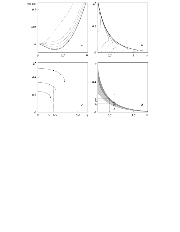
Figure 8: The total ground–state energy per site $\cal{E}(\delta)$ vs. dimerization parameter $\delta$ ($\alpha=0.5$, from bottom to top $\gamma=0,\;0.025,\;0.05,\;0.1,\;0.15,\;0.2,\;0.4$) (a), the dimerization parameter $\delta^{\star}$ vs. $\alpha$ (from right to left $\gamma=0,\;0.025,\;0.05,\;0.1,\;0.15,\;0.2,\;0.4$) (b), the dimerization parameter $\delta^{\star}$ vs. $\gamma$ (from top to bottom $\alpha=0.4,\;0.5,\;0.6$; the meaning of the characteristic values of the anisotropy parameter $\gamma_{A}$, $\gamma_{B}$, $\gamma_{C}$ (denoted for $\alpha=0.5$) is explained in the main text) (c), and the phase diagram in the plane $\alpha$ – $\gamma$ (in the region A (C) the dimerized (uniform) phase occurs; in the regions B₁, B₂ both phases are possible although in the region B₁ (B₂) the dimerized (uniform) phase is favorable) (d).

if $|\omega^{2}-\delta^{2}|\leq 1$. For the chain of period 3 Eq. (3.4) has again obvious solutions $\cos^{2}\theta_{1}=\cos^{2}\theta_{2}=\cos^{2}\theta_{3}=1$; another solution existing at a certain range of the transverse field can be found numerically (see Figs. 4j – 4l). The described analytical calculations reproduce the results obtained earlier numerically for some chains of periods 2 and 3 (dashed curves in Figs. 8a, 8b of Ref. 024, ).

In Figs. 4a – 4i we display the obtained dependences of the ground–state magnetizations $m^{z}$, $m^{x}$ and static transverse susceptibility $\chi^{z}$ on the transverse field for several classical transverse Ising/$XX$ chains of period 3 (the results for corresponding quantum chains are shown in Fig. 3). In contrast to the quantum case, the ground–state static transverse susceptibility $\chi^{z}$ of the classical chains remains always finite as the transverse field $\Omega$ varies and hence the classical chains do not exhibit any ground–state phase transitions driven by $\Omega$. However, a regularly alternating classical chain similarly to its quantum ($XX$) counterpart may exhibit plateaus in the ground–state dependence transverse magnetization $m^{z}$ vs. transverse field $\Omega$ (compare long–dashed–dotted curves in Fig. 4b (classical chain) and Fig. 3h (quantum chain) which have a plateau $-m^{z}=\frac{1}{6}$). Obviously, as $m^{z}$ remains constant with varying $\Omega$, the static transverse susceptibility is zero (long–dashed–dotted curves in Fig. 4e). Moreover, $m_{n}^{x}$ ($m_{n}^{\perp}$), $n=1,2,3$ in this region is zero (Fig. 4h) and the stable ground–state spin configuration is $\theta_{n}=\theta_{n+1}=\pi$, $\theta_{n+2}=0$ (see Fig. 4l). The Ising magnetization $m^{x}$ decays as the system runs out the Ising phase according to the power–law, $m^{x}\sim|\Omega^{\star}-\Omega|^{\beta}$, with $\beta=\frac{1}{2}$.

III.3 Quantum phase transitions

Let us have a closer look at the quantum phase transitions in regularly alternating transverse Ising chains discussing in some detail the critical behavior. For such a chain of period $p$ the quantum phase transition points are determined by Eq. (2.14). The effects of regular alternation on the number and position of the quantum phase transition points in the cases $p=2$ and $p=3$ were analyzed in Section II. Although Eq. (2.14) was found many years ago023 it was not discussed in the context of the quantum phase transition theory. In particular, an important question how the gap vanishes as the set of parameters becomes critical was not considered in Ref. 023, . Below we show that two types of critical behavior are possible: one as it occurs for the second–order phase transition (in Ehrenfest’s sense) and another one as it occurs for a weaker singularity (the fourth–order phase transition in Ehrenfest’s sense). These findings are confirmed by numerical computations of the two–site spin correlation functions.

First we analyze how the gap vanishes as the set of parameters becomes critical for the case $p=2$ when $\Omega^{\star}=\pm\sqrt{\Delta\Omega^{2}\pm|I_{1}I_{2}|}$. Eq. (II) yields

$$\Delta^{2}(\Omega)\approx\frac{\left(\Omega^{2}-{\Omega^{\star}}^{2}\right)^{2}}{2\left(\Omega^{2}+{\Delta\Omega}^{2}+\frac{I_{1}^{2}+I_{2}^{2}}{2}\right)}.$$ (3.6)

If $|\Omega-\Omega^{\star}|=\epsilon\to 0$ and $\Omega^{\star}\neq 0$ Eq. (3.6) suggests $\Delta^{2}(\Omega)\sim\epsilon^{2}$, i.e., the energy gap vanishes linearly (see Fig. 1a). A linear decay of the energy gap can be also seen in many cases in Figs. 1b – 1d for chains of period 3. The linearly vanishing gap corresponds to the square–lattice Ising model universality class for critical behavior. In particular, owing to such a decay of $\Delta$ the ground–state energy per site in the vicinity of $\Omega^{\star}$ has the form

$$e_{0}=-\int_{0}^{\infty}{\mbox{d}}EE^{2}R(E^{2})$$

$$=-\frac{1}{p\pi}\int_{\sqrt{\epsilon^{2}}}^{\sqrt{a_{2}}}{\mbox{d}}EE^{2}\frac{f(E^{2})}{\sqrt{E^{2}-\epsilon^{2}}}$$

$$+{\mbox{analytical with respect to}}\;\epsilon^{2}\;{\mbox{terms}}.$$ (3.7)

Here the first term is a contribution of the lowest energy band and the explicit expression for $f(E^{2})$ is not important for the analysis of nonanalytical behavior as $\epsilon\to 0$. The first term in (III.3) is proportional to $\epsilon^{2}\ln\epsilon$ and as a result the zero–temperature dependence of $m^{z}$ and $\chi^{z}$ on $\Omega$ contains the nonanalytical terms $\left(\Omega-\Omega^{\star}\right)\ln|\Omega-\Omega^{\star}|$ and $\ln|\Omega-\Omega^{\star}|$, respectively.

Let us turn to the case $p=2$ with $\Delta\Omega=\sqrt{|I_{1}I_{2}|}$ when we have three critical fields $\Omega^{\star}=\left\{\pm\sqrt{2|I_{1}I_{2}|},0\right\}$ and consider the behavior of $\Delta(\Omega)$ in the vicinity of $\Omega^{\star}=0$, i.e., as $\Omega\to 0$. From Eq. (3.6) one finds that $\Delta^{2}(\Omega)\sim\epsilon^{4}$. Repeating the calculation of the ground–state energy (see Eq. (III.3)) for such a decay of $\Delta$ one finds that $e_{0}$ contains the term $\epsilon^{4}\ln\epsilon$ and hence the system exhibits the fourth–order (in Ehrenfest’s sense) quantum phase transition at $\Omega^{\star}=0$ which is characterized by a logarithmic divergence of the second derivative of the susceptibility $\frac{\partial^{2}\chi^{z}}{\partial\Omega^{2}}$. (For an example of a fourth–order thermal phase transition see Ref. 027, .) For $p=3$ the dependence $\Delta(\Omega)\sim\epsilon^{2}$ (see Figs. 1b – 1d) may occur for the sets of parameters at the boundaries between different regions in Fig. 2 (e.g., at the points b, c, e). Such systems again show the fourth–order quantum phase transition behavior while approaching the corresponding critical fields.

To discuss further the quantum phases which occur as the transverse field varies we examine the spin correlation functions $\langle s_{n}^{\alpha}s_{n+l}^{\alpha}\rangle$. Unfortunately, we cannot obtain the spin correlation functions of a regularly alternating transverse Ising chain using the continued fraction approach which is restricted to the quantities that can be expressed through the density of states (2.4). However, the spin correlation functions can be determined numerically (see, for example, Ref. 028, ) for rather long chains of several thousand sites. Knowing $\langle s_{n}^{\alpha}s_{n+l}^{\alpha}\rangle$ we can obtain the on-site magnetization ${m_{n}^{\alpha}}^{2}=\mbox{lim}_{r\to\infty}\langle s_{n}^{\alpha}s_{n+rp}^{\alpha}\rangle$. Assuming that $\langle s_{n}^{\alpha}s_{n+rp}^{\alpha}\rangle-\langle s_{n}^{\alpha}\rangle\langle s_{n+rp}^{\alpha}\rangle$ decays as $\left(rp\right)^{-\gamma^{\alpha}}\exp\left(-\frac{rp}{\xi^{\alpha}}\right)$ if $r\to\infty$ we can also find the correlation length $\xi^{\alpha}$ and the power–law exponent $\gamma^{\alpha}$. In our calculations for $p=3$ we consider chains with $N=2100$, take $n=500$, $rp=999$ to determine $|m_{j}^{x}|$ and $rp=60,\ldots,360$ to determine $\xi^{x}$ and $\gamma^{x}$. Our findings are collected in Fig. 5. To illustrate the critical behavior of the order parameter in detail we also consider a chain of period 2 with $|I_{1}|=|I_{2}|=1$, $\Omega_{1,2}=\Omega\pm 1$ taking $N=2000,\;4000,\;5400$, $n=\frac{N}{4}$, $rp=\frac{N}{2}$. The zero–temperature dependences $|m^{x}_{j}|$ vs. $\Omega$ for this chain are reported in Fig. 6.

As can be seen from Figs. 5, 6 the behavior of the Ising magnetization $m^{x}$ (which plays the role of the order parameter) indicates the different phases (Ising phase if $m^{x}\neq 0$ or paramagnetic phase if $m^{x}=0$) and the phase transitions between them. For a set of parameters which yields weak singularities (i.e., $m^{x}=0$ in the Ising phase, see Figs. 5b, 5c, 5e, 6a, 6b) the finite–size effects are strong and the finite–chain result for $x$–magnetization tends to zero very slowly with increasing $N$ (compare data for different $N$ in Fig. 6b). For the second–order (fourth–order) quantum phase transition points the critical behavior is given by $m^{x}\sim|\Omega^{\star}-\Omega|^{\beta}$ with $\beta=\frac{1}{8}$ ($\beta=\frac{1}{4}$) (compare Figs. 6c and 6b). The appearance/disappearance of the Ising magnetization is accompanied by a divergence of the correlation length $\xi^{x}=|\Omega-\Omega^{\star}|^{-\nu}$ with $\nu=1$ ($\nu=2$) for the second–order (fourth–order) quantum phase transition points (Figs. 5g – 5l). Taking into account the values of the exponent characterizing the energy gap behavior we conclude that the relaxation time scales like the first power of the correlation length, i.e., the dynamic exponent $z=1$, for both the second–order and the fourth–order quantum phase transitions. At $\Omega=\Omega^{\star}$ the $xx$ spin correlation functions show power–law decay with the exponent $\gamma^{x}=\frac{1}{4}$ for both the second–order and the fourth–order quantum phase transitions (Figs. 5m – 5r). Finally, the results for spin correlation functions at special values of the transverse field $\Omega$, i.e., when one on–site field equals zero, coincide with the analytical predictions obtained using the 3–site cluster Hamiltonian eigenvectors (for a chain of period 2 the corresponding calculations are given in Ref. 029, ). For example, for the chain of period 3 with $I_{1}=I_{2}=I_{3}=1$, $\Delta\Omega_{1}=1$, $\Delta\Omega_{2}=0$, $\Delta\Omega_{3}=-1$ at $\Omega=-1$ we have found $|m_{1}^{x}|=\frac{1}{2},\;\;\;|m_{2}^{x}|\approx 0.417,\;\;\;|m_{3}^{x}|\approx 0.331$ (see Fig. 5a) whereas for such a chain with $\Delta\Omega_{1}=2$, $\Delta\Omega_{2}=0$, $\Delta\Omega_{3}=-2$ at $\Omega=-2$ we have found $|m_{1}^{x}|=\frac{1}{2},\;\;\;|m_{2}^{x}|\approx 0.267,\;\;\;|m_{3}^{x}|\approx 0.175$ (see Fig. 5f). It should be noted that the Ising magnetization at the sites with zero transverse fields has its maximal value $\frac{1}{2}$. Probably the most spectacular feature of the Ising chain with regularly alternating transverse field is the reentrant behavior with varying $\Omega$ nicely seen in Figs. 5d – 5f. The appearance of the paramagnetic phase at intermediate values of the transverse field when $x$–magnetization is zero and $z$–magnetization is almost constant can be associated with the following classical picture. Assume, for example, $p=2$ and $\Omega=0$; then owing to the regularly varying on–site transverse fields $\pm\Delta\Omega$ with large $\Delta\Omega$ all on–site magnetizations are directed in $\pm z$–direction in the spin space. Naturally, this picture may play only an auxiliary role for the considered quantum systems.

Finally we note that our results are in agreement with the scaling relations in the theory of conventional (temperature–driven) phase transitions030 . Thus, the quantum phase transition in dimension $d=1$ corresponds to the thermal phase transition in dimension $d+z=2$, the exponent $\nu$ which characterizes the divergence of the correlation length $\xi\sim|T-T_{c}|^{-\nu}$ characterizes the decay of the energy gap $\Delta\sim|\Omega-\Omega^{\star}|^{\nu}$, the exponent $\alpha$ characterizing the divergence of the specific heat $c\sim|T-T_{c}|^{-\alpha}$ characterizes the divergence of the transverse susceptibility $\chi^{z}\sim|\Omega-\Omega^{\star}|^{-\alpha}$. Moreover, a number of scaling relations (which do not account for logarithmic divergences) hold. For example, $2-\alpha=d\nu$. Substituting $d=2$, $\nu=1$ one gets $\alpha=0$, i.e., only a logarithmic divergence in the dependence $\chi^{z}$ vs. $\Omega$, whereas for more rapidly decaying energy gap when $\nu=2$ one finds $\alpha=-2$, i.e., $\chi^{z}$ does not diverge at $\Omega^{\star}$ (and only its second derivative exhibits a logarithmic peculiarity).

III.4 Temperature behavior of the specific heat

We turn to a discussion of the effects of regular alternation on the temperature dependence of the specific heat. The low–temperature behavior of this quantity is determined by the fact whether the system is gapped or gapless. Thus, the zero–energy excitations immediately produce a linear dependence of the specific heat on temperature. As a result the low–temperature behavior of the specific heat indicates the quantum phase transition points that can be seen in Fig. 7 in complete agreement with the outcomes which follow from the behavior of the $xx$ spin correlation functions shown in Fig. 5. Moreover, we notice that the regular alternation may produce many–peak structure of the temperature profiles of the specific heat (Fig. 7).

IV Anisotropic $XY$ chain without field. Spin–Peierls dimerization

As a byproduct of the study of regularly alternating transverse Ising chains we obtain the thermodynamic quantities of regularly alternating anisotropic $XY$ chains without field (1.3). Really, using the unitary transformations discussed in the end of Section I we can state that the Helmholtz free energy of the regularly alternating anisotropic $XY$ chain without field (1.3) defined by a sequence of parameters $I_{1}^{x}I_{1}^{y}I_{2}^{x}I_{2}^{y}\ldots I_{p}^{x}I_{p}^{y}I_{1}^{x}I_{1}^{y}I_{2}^{x}I_{2}^{y}\ldots I_{p}^{x}I_{p}^{y}\ldots$ is given by Eq. (2.5) with $R(E^{2})$ (2.7) and the diagonal Green functions involved into Eq. (2.7) are determined as follows

$$G_{nn}=\frac{1}{E^{2}-{I^{x}_{n-1}}^{2}-{I^{y}_{n}}^{2}-\Delta_{n}^{-}-\Delta_{n}^{+}},$$ (4.1)

$$\Delta_{n}^{-}=\frac{{I^{y}_{n-2}}^{2}{I^{x}_{n-1}}^{2}}{E^{2}-{I^{x}_{n-3}}^{2}-{I^{y}_{n-2}}^{2}-\frac{{I^{y}_{n-4}}^{2}{I^{x}_{n-3}}^{2}}{E^{2}-{I^{x}_{n-5}}^{2}-{I^{y}_{n-4}}^{2}-_{\ddots}}},$$

$$\Delta_{n}^{+}=\frac{{I^{y}_{n}}^{2}{I^{x}_{n+1}}^{2}}{E^{2}-{I^{x}_{n+1}}^{2}-{I^{y}_{n+2}}^{2}-\frac{{I^{y}_{n+2}}^{2}{I^{x}_{n+3}}^{2}}{E^{2}-{I^{x}_{n+3}}^{2}-{I^{y}_{n+4}}^{2}-_{\ddots}}}.$$

Moreover, we may use the obtained densities of states (2.11), (II), (II) to find the thermodynamic quantities of some regularly alternating anisotropic $XY$ chains. Thus, the anisotropic $XY$ chain of period 2 is unitary equivalent to two different transverse Ising chains both of period 1 and as a result

$$R(E^{2})=\left\{\begin{array}[]{ll}\frac{1}{2\pi}\frac{1}{\sqrt{{\cal{A}}_{xy}(E^{2})}},&{\mbox{if}}\;\;\;{\cal{A}}_{xy}(E^{2})>0\\ 0,&{\mbox{otherwise}}\end{array}\right.$$ (4.4)

$$+\left\{\begin{array}[]{ll}\frac{1}{2\pi}\frac{1}{\sqrt{{\cal{A}}_{yx}(E^{2})}},&{\mbox{if}}\;\;\;{\cal{A}}_{yx}(E^{2})>0,\\ 0,&{\mbox{otherwise}},\end{array}\right.$$ (4.7)

$${\cal{A}}_{\alpha\beta}(E^{2})=-\left(E^{2}-\left(I_{1}^{\alpha}-I_{2}^{\beta}\right)^{2}\right)\left(E^{2}-\left(I_{1}^{\alpha}+I_{2}^{\beta}\right)^{2}\right).$$

(Note, that for the isotropic case $I_{1}^{x}=I_{1}^{y}=I_{1}$, $I_{2}^{x}=I_{2}^{y}=I_{2}$, Eq. (4.4) yields the result obtained in Ref. 024, (Eqs. (9) – (11) of that paper); in the anisotropic case Eq. (4.4) agrees with the result reported in Ref. 010, .) The anisotropic $XY$ chain of period 3 after performing the above mentioned unitary transformations is equivalent to two identical transverse Ising chains of period 3 and, therefore, $R(E^{2})$ is given by Eqs. (2.11), (II) after the substitution $\Omega_{1}\to I_{1}^{y}$, $I_{1}\to I_{2}^{x}$, $\Omega_{2}\to I_{3}^{y}$, $I_{2}\to I_{1}^{x}$, $\Omega_{3}\to I_{2}^{y}$, $I_{3}\to I_{3}^{x}$. Let us also note that the anisotropic $XY$ chains of period 4 (6) are unitary equivalent to two different transverse Ising chains of period 2 (3) and hence after simple substitutions Eqs. (2.11), (II) (Eqs. (2.11), (II)) yield the thermodynamic properties of such chains.

Let us use the ground–state energy per site $e_{0}=-2\int_{0}^{\infty}{\mbox{d}}EE^{2}R(E^{2})$ of the anisotropic $XY$ chain of period 2 to examine the effects of the exchange interaction anisotropy on the spin–Peierls dimerization inherent in the isotropic $XY$ chain031 ; 032 . For this purpose we assume in (4.4) $I_{1}^{x}=(1+\delta)(1+\gamma)$, $I_{1}^{y}=(1+\delta)(1-\gamma)$, $I_{2}^{x}=(1-\delta)(1+\gamma)$, $I_{2}^{y}=(1-\delta)(1-\gamma)$ where $0\leq\delta<1$ is the dimerization parameter and $0\leq\gamma\leq 1$ is the exchange interaction anisotropy parameter. We consider the total energy per site ${\cal{E}}(\delta)$ and its dependence on $\delta$. ${\cal{E}}(\delta)$ consists of the magnetic part $e_{0}(\delta)$ and the elastic part $\alpha\delta^{2}$. Let us recall that in the isotropic limit $\gamma=0$ the total energy ${\cal{E}}(\delta)$ exhibits a minimum at a nonzero value of the dimerization parameter $\delta^{\star}\neq 0$ which is a manifestation of lattice instability with respect to spin–Peierls dimerization031 . In the other limiting case $\gamma=1$ the magnetic energy does not depend on $\delta$ and hence the uniform lattice is stable. In Fig. 8a one can see how the behavior of ${\cal{E}}(\delta)$ vs. $\delta$ varies as $\gamma$ increases from 0 to 0.4 for $\alpha=0.5$. At $\gamma=0$ the total energy ${\cal{E}}(\delta)$ exhibits a minimum at a nonzero value of dimerization parameter $\delta^{\star}\neq 0$. As $\gamma$ increases the dependence remains qualitatively the same with, however, slightly decreasing value of $\delta^{\star}$ (see Figs. 8b and 8c). At a certain value of anisotropy parameter $\gamma_{A}$ an additional minimum at $\delta=0$ appears. Both minima are separated by a maximum, and the minimum at $\delta^{\star}\neq 0$ remains the deeper one. At the value of $\gamma_{B}$ ($>\gamma_{A}$) the minima have the same depth and with further increase of $\gamma$ the minimum at $\delta=0$ becomes the deeper one. If $\gamma$ exceeds $\gamma_{C}$ ($>\gamma_{B}$) the minimum for a nonzero dimerization parameter disappears. In Fig. 8b one can see the behavior of $\delta^{\star}$ as $\gamma$ varies from 0 to 0.4 for different $\alpha$s (solid curves; the dashed curves show the behavior of the maximum in the dependence ${\cal{E}}(\delta)$ vs. $\delta$); in Fig 8c one can see the dependence of $\delta^{\star}$ on $\gamma$ for $\alpha=0.4,\;0.5,\;0.6$. The bold dots in the curves in this panel correspond to the characteristic values of the anisotropy parameter $\gamma_{A}<\gamma_{B}<\gamma_{C}$ discussed above. The effect of the anisotropy on the spin–Peierls dimerized phase occurs according to the first–order phase transition scenario. The corresponding phase diagram is shown in Fig. 8d where we indicate the region of stability of the dimerized (A) and uniform (C) phases as well as the metastable region (regions B₁ and B₂) where both phases may coexist.

It is interesting to compare the described effects of the exchange interaction anisotropy on the spin–Peierls dimerized phase with the effects of the transverse field on the spin–Peierls dimerized phase032 ; 024 . Similarly to the anisotropy $\gamma$ the transverse field $\Omega$ destroys the dimerized phase according to a first–order phase transition scenario. However, the value of the dimerization parameter $\delta^{\star}$ remains unchanged as $\Omega$ increases up to $\Omega_{C}$.

V Concluding remarks

In this work we have analyzed in some detail the ground–state and thermodynamic properties of regularly alternating spin–$\frac{1}{2}$ transverse Ising chains and anisotropic $XY$ chains without field. Due to the Jordan–Wigner mapping and the continued fraction approach we can calculate the thermodynamic quantities rigorously analytically. For certain values of parameters we can also calculate the ground–state spin correlation functions. For other values of parameters we have calculated the spin correlation functions numerically for long chains consisting of a few thousand sites. We have shown how the ground–state properties of regularly alternating classical transverse Ising/$XX$ chains can be examined. The main new results obtained are as follows. Firstly, we have examined the effects of regular alternation on quantum phases and quantum phase transitions in the transverse Ising chain. Owing to regularly alternating parameters the number of quantum phase transition may increase (but never exceeds $2p$ where $p$ is the period of alternation), the critical behavior remains as in the uniform chain, however, a weaker singularity may also appear. Secondly, we have demonstrated how the plateaus in the ground–state magnetization curves for the classical regularly alternating transverse Ising/$XX$ chains may emerge. Thirdly, we have shown how the exchange interaction anisotropy destroys the spin–Peierls dimerization inherent in the spin–$\frac{1}{2}$ isotropic $XY$ chain. The performed study provides a set of reference results which may be useful for understanding more complicated quantum spin chains.

Figure 1: The energy gap $\Delta$ vs. transverse field $\Omega$ for transverse Ising chains of period 2 (panel a) and 3 (panels b – d) ($\Omega_{n}=\Omega+\Delta\Omega_{n}$, $\sum_{n=1}^{p}\Delta\Omega_{n}=0$, $I_{n}=1$; $\Delta\Omega_{2}=\Delta\Omega_{1}$ (b), $\Delta\Omega_{2}=\frac{1}{2}\Delta\Omega_{1}$ (c), $\Delta\Omega_{2}=-\Delta\Omega_{1}$ (d)). The bold curves $\Delta$ vs. $\Omega$ correspond to the following values of parameters: $\Delta\Omega_{1}=0.5,\;1,\;1.5$ (panel a), $\Delta\Omega_{1}=0.5$, $\Delta\Omega_{1}\approx 0.630$, $\Delta\Omega_{1}=1$ (panel b), $\Delta\Omega_{1}=0.5$, $\Delta\Omega_{1}\approx 0.848$, $\Delta\Omega_{1}=1.5$, $\Delta\Omega_{1}\approx 1.921$ (panel c), $\Delta\Omega_{1}=1$, $\Delta\Omega_{1}\approx 1.375$, $\Delta\Omega_{1}=2$ (panel d). The bold curves in the plane $\Omega$–$\Delta\Omega_{1}$ indicate the values of parameters which yield the zero–energy gap, $\Delta=0$.

Figure 2: Phase diagram of the transverse Ising chain of period 3 with $|I_{1}I_{2}I_{3}|=1$, $\Omega_{1,2,3}=\Omega+\Delta\Omega_{1,2,3}$, $\Delta\Omega_{1}+\Delta\Omega_{2}+\Delta\Omega_{3}=0$. As $\Omega$ varies the energy gap vanishes two/four/six times if the set of parameters is in the dark/gray/light region. The sets of parameters denoted by a, b, c, d, e, f are used below to illustrate the dependence on $\Omega$ of the ground–state Ising magnetization (Fig. 5) and the low–temperature specific heat (Fig. 7).

Figure 3: The ground–state transverse magnetization (a, b, c, g, h, i) and static transverse susceptibility (d, e, f, j, k, l) curves for transverse Ising (a – f) and transverse $XX$ (g – l) chains of period $p=3$. $I_{1,2,3}=1$, $\Omega_{1,2,3}=\Omega+\Delta\Omega_{1,2,3}$, $\Delta\Omega_{1}+\Delta\Omega_{2}+\Delta\Omega_{3}=0$; a, d, g, j: $\Delta\Omega_{2}=\Delta\Omega_{1}$, $\Delta\Omega_{1}=0$ (solid curves), $\Delta\Omega_{1}=0.5$ (long–dashed curves), $\Delta\Omega_{1}=0.6$ (short–dashed curves), $\Delta\Omega_{1}=1$ (dotted curves); b, e, h, k: $\Delta\Omega_{2}=\frac{1}{2}\Delta\Omega_{1}$, $\Delta\Omega_{1}=0$ (solid curves), $\Delta\Omega_{1}=0.5$ (long–dashed curves), $\Delta\Omega_{1}=0.85$ (short–dashed curves), $\Delta\Omega_{1}=1.5$ (dotted curves), $\Delta\Omega_{1}=1.9$ (long–dashed–dotted curves); c, f, i, l: $\Delta\Omega_{2}=-\Delta\Omega_{1}$, $\Delta\Omega_{1}=0$ (solid curves), $\Delta\Omega_{1}=1$ (long–dashed curves), $\Delta\Omega_{1}=1.35$ (short–dashed curves), $\Delta\Omega_{1}=2$ (dotted curves).

Figure 4: The ground–state transverse magnetization (a, b, c), Ising magnetization (g, h, i), and static transverse susceptibility (d, e, f) curves for the classical transverse Ising/$XX$ chains of period $p=3$. $I_{1,2,3}=-1$, $\Omega_{1,2,3}=\Omega+\Delta\Omega_{1,2,3}$, $\Delta\Omega_{1}+\Delta\Omega_{2}+\Delta\Omega_{3}=0$; a, d, g: $\Delta\Omega_{2}=\Delta\Omega_{1}$, $\Delta\Omega_{1}=0$ (solid curves), $\Delta\Omega_{1}=0.5$ (long–dashed curves), $\Delta\Omega_{1}=0.6$ (short–dashed curves), $\Delta\Omega_{1}=1$ (dotted curves); b, e, h: $\Delta\Omega_{2}=\frac{1}{2}\Delta\Omega_{1}$, $\Delta\Omega_{1}=0$ (solid curves), $\Delta\Omega_{1}=0.5$ (long–dashed curves), $\Delta\Omega_{1}=0.85$ (short–dashed curves), $\Delta\Omega_{1}=1.5$ (dotted curves), $\Delta\Omega_{1}=1.9$ (long–dashed–dotted curves); c, f, i: $\Delta\Omega_{2}=-\Delta\Omega_{1}$, $\Delta\Omega_{1}=0$ (solid curves), $\Delta\Omega_{1}=1$ (long–dashed curves), $\Delta\Omega_{1}=1.35$ (short–dashed curves), $\Delta\Omega_{1}=2$ (dotted curves). We also show the ground–state spin configurations $\theta_{1}$, $\theta_{2}$, $\theta_{3}$ (the corresponding curves are denoted by 1, 2, 3) for the chains with $\Delta\Omega_{2}=\frac{1}{2}\Delta\Omega_{1}$ (see panels b, e, h) and $\Delta\Omega_{1}=0.85$ (j), $\Delta\Omega_{1}=1.5$ (k), $\Delta\Omega_{1}=1.9$ (l) as $\Omega$ varies.

Figure 5: The ground–state $x$–magnetization $m^{x}=\frac{1}{3}\left(|m_{1}^{x}|+|m_{2}^{x}|+|m_{3}^{x}|\right)$ (a, b, c, d, e, f), inverse correlation length $\frac{1}{\xi^{x}}$ (g, h, i, j, k, l), and $\gamma^{x}$ (m, n, o, p, q, r) for the transverse Ising chain of period 3 with $|I_{1}|=|I_{2}|=|I_{3}|=1$, $\Omega_{1,2,3}=\Omega+\Delta\Omega_{1,2,3}$, $\Delta\Omega_{1}+\Delta\Omega_{2}+\Delta\Omega_{3}=0$, $\Delta\Omega_{1}=1$, $\Delta\Omega_{2}=0$ ($\Omega^{\star}\approx\left\{\pm 1.325\right\}$) (a, g, m), $\Delta\Omega_{1}=1$, $\Delta\Omega_{2}\approx 0.292$ ($\Omega^{\star}\approx\left\{-1.355,0.678,1.513\right\}$) (b, h, n), $\Delta\Omega_{1}=\left(\frac{27}{4}\right)^{\frac{1}{6}}\approx 1.374$, $\Delta\Omega_{2}=0$ ($\Omega^{\star}\approx\left\{\pm 0.794,\pm 1.587\right\}$) (c, i, o), $\Delta\Omega_{1}=\left(\frac{27}{4}\right)^{\frac{1}{6}}\approx 1.374$, $\Delta\Omega_{2}=-1$ ($\Omega^{\star}\approx\left\{-1.574,-1.020,-0.348,1.367\right\}$) (d, j, p), $\Delta\Omega_{1}=2$, $\Delta\Omega_{2}\approx-1.575$ ($\Omega^{\star}\approx\left\{-2.107,-1.874,0.102,1.054,1.772\right\}$) (e, k, q), $\Delta\Omega_{1}=2$, $\Delta\Omega_{2}=0$ ($\Omega^{\star}\approx\left\{\pm 0.254,\pm 1.861,\pm 2.115\right\}$) (f, l, r). Connecting curves are guides to the eye. The taken sets of parameters are in correspondence with the points a, b, c, d, e, f in Fig. 2.

Figure 6: The ground–state sublattice $x$–magnetizations $|m_{j}^{x}|$, $j=1,2$ (triangles) and $m^{x}=\frac{1}{2}\left(|m_{1}^{x}|+|m_{2}^{x}|\right)$ (squares, diamonds, circles) for the transverse Ising chain of period 2 with $|I_{1}|=|I_{2}|=1$, $\Omega_{1,2}=\Omega\pm 1$. Connecting curves in panel a are guides to the eye. We also report the results for the dependence $m^{x}$ vs. $\Omega$ in the vicinity of the critical points $\Omega^{\star}=0$ (b) and $\Omega^{\star}=\sqrt{2}$ (c) (squares, diamonds, circles correspond to data for $N=2000,\;4000,\;5400$, respectively, solid lines represent dependences $\sim\Omega^{\frac{1}{4}}$ (b) and $\sim\left(\sqrt{2}-\Omega\right)^{\frac{1}{8}}$ (c)).

Figure 7: The low–temperature behavior of the specific heat for the transverse Ising chain of period 3 with $|I_{1}|=|I_{2}|=|I_{3}|=1$, $\Omega_{1,2,3}=\Omega+\Delta\Omega_{1,2,3}$, $\Delta\Omega_{1}+\Delta\Omega_{2}+\Delta\Omega_{3}=0$, $\Delta\Omega_{1}=1$, $\Delta\Omega_{2}=0$ (a), $\Delta\Omega_{1}=1$, $\Delta\Omega_{2}\approx 0.292$ (b), $\Delta\Omega_{1}\approx 1.374$, $\Delta\Omega_{2}=0$ (c), $\Delta\Omega_{1}\approx 1.374$, $\Delta\Omega_{2}=-1$ (d), $\Delta\Omega_{1}=2$, $\Delta\Omega_{2}\approx-1.575$ (e), $\Delta\Omega_{1}=2$, $\Delta\Omega_{2}=0$ (f).

References

- (1) E. Lieb, T. Schultz, and D. Mattis, Ann. Phys. (N.Y.) 16, 407 (1961).
- (2) E. Fradkin, Field Theories of Condensed Matter Systems (Addison–Wesley Publishing Company: Redwood City, California Menlo Park, California Reading, Massachusetts New York Don Mills, Ontario Workingham, United Kingdom Amsterdam Bonn Sydney Singapore Tokyo Madrid San Juan, 1991).
- (3) B. K. Chakrabarti, A. Dutta, and P. Sen, Quantum Ising Phases and Transitions in Transverse Ising Models (Springer–Verlag: Berlin Heidelberg, 1996).
- (4) S. Sachdev, Quantum Phase Transitions (Cambridge University Press: Cambridge New York Melbourne Madrid, 1999).
- (5) P. Pfeuty, Ann. Phys. (N.Y.) 57, 79 (1970).
- (6) J. M. Luck, J. Stat. Phys. 72, 417 (1993).
-
(7)
D. S. Fisher,
Phys. Rev. Lett. 69, 534 (1992);
D. S. Fisher, Phys. Rev. B 51, 6411 (1995). - (8) F. Iglói, L. Turban, D. Karevski, and F. Szalma, Phys. Rev. B 56, 11031 (1997).
- (9) Jong–Won Lieh, J. Math. Phys. 11, 2114 (1970).
- (10) J. H. H. Perk, H. W. Capel, M. J. Zuilhof, and Th. J. Siskens, Physica A 81, 319 (1975).
- (11) K. Okamoto and K. Yasumura, J. Phys. Soc. Jap. 59, 993 (1990).
- (12) L. L. Gonçalves and J. P. de Lima, J. Phys.: Condens. Matter 9, 3447 (1997).
- (13) F. F. B. Filho, J. P. de Lima, and L. L. Gonçalves, J. Magn. Magn. Mater. 226–230, 638 (2001).
- (14) P. Tong and M. Zhong, Physica B 304, 91 (2001).
- (15) F. Ye, G. – H. Ding, and B. – W. Xu, cond-mat/0105584.
- (16) M. Arlego, D. C. Cabra, J. E. Drut, and M. D. Grynberg, Phys. Rev. B 67, 144426 (2003).
-
(17)
O. Derzhko,
J. Phys. A 33, 8627 (2000);
O. Derzhko, Czechoslovak Journal of Physics 52, A277 (2002). - (18) D. C. Mattis, The Theory of Magnetism II. Thermodynamics and Statistical Mechanics (Springer–Verlag: Berlin Heidelberg New York Tokyo, 1985).
- (19) H. Braeter and J. M. Kowalski, Physica A 87, 243 (1977).
- (20) P. Henelius and S. M. Girvin, Phys. Rev. B 57, 11457 (1998).
-
(21)
O. V. Derzhko and T. Ye. Krokhmalskii,
Visn. L’viv. Univ., Ser. Fiz. (L’viv) 26, 47 (1993)
(in Ukrainian);
O. Derzhko and T. Krokhmalskii, Ferroelectrics 153, 55 (1994). - (22) J. Slechta, J. Phys. C 10, 2047 (1977).
- (23) P. Pfeuty, Phys. Lett. A 72, 245 (1979).
- (24) O. Derzhko, J. Richter, and O. Zaburannyi, Physica A 282, 495 (2000).
- (25) J. P. de Lima and L. L. Gonçalves, J. Magn. Magn. Mater. 206, 135 (1999).
- (26) G. S. Joyce, Phys. Rev. 155, 478 (1967).
-
(27)
P. Kumar, D. Hall, and R. G. Goodrich,
Phys. Rev. Lett. 82, 4532 (1999);
P. Kumar, cond-mat/0207373. -
(28)
O. Derzhko and T. Krokhmalskii,
Phys. Rev. B 56, 11659 (1997);
O. Derzhko and T. Krokhmalskii, physica status solidi (b) 208, 221 (1998). -
(29)
O. Derzhko, J. Richter, T. Krokhmalskii, and O. Zaburannyi,
Phys. Rev. B 66, 144401 (2002);
O. Derzhko, J. Richter, T. Krokhmalskii, and O. Zaburannyi, Acta Physica Polonica B 34, 1387 (2003). - (30) S. – K. Ma, Modern Theory of Critical Phenomena (Addison-Wesley Publishing: Reading, Mass., London, Benjamin, 1976).
- (31) P. Pincus, Solid State Commun. 9, 1971 (1971).
- (32) J. H. Taylor and G. Müller, Physica A 130, 1 (1985).