Coherent rotations of a single spin-based qubit in a single quantum dot at fixed Zeeman energy

Abstract

Coherent rotations of single spin-based qubits may be accomplished electrically at fixed Zeeman energy with a qubit defined solely within a single electrostatically-defined quantum dot; the $g$-factor and the external magnetic field are kept constant. All that is required to be varied are the voltages on metallic gates which effectively change the shape of the elliptic quantum dot. The pseudospin-1/2 qubit is constructed from the two-dimensional $S=1/2$, $S_{z}=-1/2$ subspace of three interacting electrons in a two-dimensional potential well. Rotations are created by altering the direction of the pseudomagnetic field through changes in the shape of the confinement potential. By deriving an exact analytic solution to the long-range Coulomb interaction matrix elements, we calculate explicitly the range of magnitudes and directions the pseudomagnetic field can take. Numerical estimates are given for GaAs.

I Introduction

The issue of real-time coherent control of individual quantum states is central to quantum computing and to many other ideas in the burgeoning field of quantum nanoelectronics. The main challenge is to isolate a system (or the interesting parts of a system) from its environment in order to prevent decoherence, yet have it environmentally coupled enough in order to perform measurements to determine what state (or distribution of states) the system is in. In a solid state system—semiconductors in particular—encoding information in the spin, rather than the charge, of an electron is a promising path since spin couples more weakly to the environment than does charge. But precisely because of this weaker environmental coupling, controlling (and measuring) the dynamics through external fields is slower and more problematic than in charge systems.

For quantum computing, employing the spin as the basic qubit, for essentially the reasons mentioned above, was recognized early on.Loss and DiVincenzo (1998) Here, the two-qubit gates are controlled electrically,Burkard et al. (1999) but single qubit rotations—a necessary ingredient in universal quantum computing—require local fields (or, more precisely, local Zeeman tuning), and necessitates breaking the spin symmetry explicitly. In contrast, one can define coded qubits;Bacon et al. (2000); Kempe et al. (2001) rather than defining a logical qubit as being a single electron (or excess electron) in a single quantum dot, a single logical qubit may be defined, for example, as several quantum dots. Explicit gate sequences Divincenzo et al. (2000) for three electrons respectively confined to three quantum dots explicitly show that the exchange interaction, controlled through gates (i.e., electrical means) alone is sufficient. This requires both additional gates and an order-of magnitude increase in gate operations.

In the present paper, we show how a spin-based qubit, defined in a single quantum dot, may be manipulated exclusively by pulsing voltages applied to gates; the external magnetic field and the $g$-factor are uniform, isotropic, and static. Thus, both single- and double-qubit gates can be constructed solely through voltage pulsing with a homogeneous, static Zeeman energy.

II Summary

Our qubit is encoded in the two-dimensional $S=1/2$, $S_{z}=-1/2$ subspace of three interacting electrons in a two-dimensional potential well. Rotations are created by tuning the eccentricity of the elliptic confinement potential.

Any two-level system can be described as a pseudospin-1/2 object in a pseudomagnetic field with a Hamiltonian written as

$$\hat{H}_{\text{qubit}}=b_{x}\hat{\sigma}_{x}+b_{y}\hat{\sigma}_{y}+b_{z}\hat{\sigma}_{z}.$$ (1)

(The most general Hamiltonian will have an additional term proportional to the identity operator.) The $\hat{\sigma}_{i}$ are the Pauli spin matrices, and the $b_{i}$ are parameters dependent upon the details of the problem. To rotate qubits, at least one of the three pseudofield components must be tunable; in principle, this degree of control can be arbitrarily small. As shown below, the pseudofield for the present system lies in a plane, which we take to be the $x$-$z$ plane ($b_{y}=0$). In particular, we consider pseudofield switching between two values, $\boldsymbol{b}_{0}$ and $\boldsymbol{b}_{1}$, which differ in magnitude and in direction $\theta$.

The crucial point demonstrated below is that the Hamiltonian of Eq. (1) may be realized in a single elliptic quantum dot, where $b_{x}$, $b_{y}$, and $b_{z}$ all have a different functional dependence on the eccentricity of the quantum dot.iso Since this eccentricity is tunable by external gates,Kyriakidis et al. (2002) the spin-based qubit may be rotated solely through external gate potentials which are local to the quantum dot.

Although our results below are for two-dimensional elliptic confinement, the general scheme holds equally well for any anisotropic (non-circular) confinement potential. The general requirements are guided by three considerations. First, the two qubit states $|0\rangle$ and $|1\rangle$ should both have the same spin ($1/2$) and spin projection. Second, if the two states differ by at least one spin-flipped pair, the relaxation should then be governed by the spin (rather than charge) relaxation time, regardless of the orbital configurations. Third, if those spin-1/2 states which define the qubit are the two lowest-energy states, then one can serve as the initial state, prepared by equilibration.

In the following section, we outline an exact solution to the one-body problem. This solution has been published before,Madhav and Chakraborty (1994) but we provide an alternate derivation based on Bose operators, similar to the circular case, which will facilitate the second-quantized treatment with interactions.

In section IV, we consider interactions. We provide, for the first time, an exact, closed-form expression for all Coulomb matrix elements (in the single-particle eigenbasis), valid for arbitrary quantum numbers.

We next detail the explicit construction of our qubit in section V, and derive Eq. (1), giving expressions for the pseudofields in terms of the various exchange energies, and, ultimately, in terms of the parameters appearing in the electronic Hamiltonian.

Following this, we give an explicit sequence of confinement deformations which enables a qubit flip and give estimates based on GaAs lateral dots using realistic potential and material parameters.

III One-body Hamiltonian: Exact solution

The Hamiltonian for a noninteracting elliptic quantum dot is given by

$$\hat{H}=\frac{1}{2m}\left(\hat{\boldsymbol{p}}-\frac{e}{c}\hat{\boldsymbol{A}}\right)^{2}+\frac{1}{2}m\left(\omega_{x}^{2}\hat{x}^{2}+\omega_{y}^{2}\hat{y}^{2}\right).$$ (2)

We have neglected the Zeeman term since it plays no significant role in what follows. Equation (2) describes one electron trapped in a plane, under a perpendicular magnetic field—we use the symmetric gauge, $\hat{\boldsymbol{A}}\equiv B(-\hat{y},\hat{x},0)/2$—with further lateral confinement by two different parabolic potentials with frequencies $\omega_{x}$ and $\omega_{y}$. This describes an elliptic confinement with the rotational symmetry (and consequent angular-momentum conservation) explicitly broken.

Equation (2) may be diagonalized by introducing Bose operators analogous to the isotropic case. (For an alternative but equivalent solution to the elliptic one-body problem, see Ref. Madhav and Chakraborty, 1994). These operators are explicitly given by

$$\begin{pmatrix}\hat{a}_{1}\\ \hat{a}_{2}^{\dagger}\end{pmatrix}=\frac{1}{\sqrt{2}}\left[\mathsf{X}\mathsf{Y}^{T}\begin{pmatrix}\hat{x}/2\ell_{0}\\ \hat{p}_{y}\ell_{0}/\hbar\end{pmatrix}+i\mathsf{X}^{-1}\mathsf{Y}\begin{pmatrix}\hat{p}_{x}\ell_{0}/\hbar\\ \hat{y}/2\ell_{0}\end{pmatrix}\right],$$ (3a)

$$\mathsf{X}=\begin{pmatrix}\alpha_{+}&0\\ 0&1/\alpha_{-}\end{pmatrix},\quad\quad\mathsf{Y}=\begin{pmatrix}\beta_{+}&\beta_{-}\\ -\beta_{-}&\beta_{+}\end{pmatrix},$$ (3b)

from which the adjoint operators $(\hat{a}_{1}^{\dagger},\ \hat{a}_{2})$ can easily be found. These four operators satisfy the canonical Boson commutation relations. The dimensionless parameters $\alpha_{\pm}$, $\beta_{\pm}$ are defined by

$$\alpha_{\pm}=\left(\frac{\omega_{0}^{2}\pm\left(\Omega^{2}+\omega_{-}^{2}\right)}{\omega_{0}^{2}\pm\left(\Omega^{2}-\omega_{-}^{2}\right)}\right)^{1/4},$$ (4a)

$$\beta_{\pm}=\left(1\pm\frac{\omega_{-}^{2}}{\Omega^{2}}\right)^{1/2},$$ (4b)

and we have also defined the (hybrid) magnetic length $\ell_{0}^{2}=\hbar/(m\omega_{0})$, cyclotron frequency $\omega_{c}=eB/(mc)$, as well as wxw

$$\omega_{0}=\left[\omega_{c}^{2}+2\left(\omega_{x}^{2}+\omega_{y}^{2}\right)\right]^{1/2},\quad\omega_{-}=\left(\omega_{x}^{2}-\omega_{y}^{2}\right)^{1/2},$$ (5)

$$\Omega=\left(\omega_{-}^{4}+\omega_{c}^{2}\omega_{0}^{2}\right)^{1/4}.$$ (6)

The Bose operators of Eq. (3) diagonalize the elliptic Hamiltonian, Eq. (2):

$$\hat{H}=\hbar\Omega_{+}\left(\hat{a}_{1}^{\dagger}\hat{a}_{1}+\frac{1}{2}\right)+\hbar\Omega_{-}\left(\hat{a}_{2}^{\dagger}\hat{a}_{2}+\frac{1}{2}\right),$$ (7)

where $\Omega_{\pm}=\frac{1}{2}\sqrt{\omega_{0}^{2}+\omega_{c}^{2}\pm 2\Omega^{2}}$. (In the isotropic limit of $\omega_{x}\rightarrow\omega_{y}$, we have $\alpha_{\pm}\longrightarrow 1$ and $\beta_{\pm}\longrightarrow 1$. The Bose operators and the Hamiltonian then reduce to the usual isotropic ones.Jacak et al. (1997))

IV Coulomb matrix elements: Exact solution

For the electron interactions, we use the long-range Coulomb energy ($\sim 1/r$) and work in the second quantized formalism using the exact single-particle basis $|mn\rangle$ ($\hat{a}_{1}^{\dagger}\hat{a}_{1}|mn\rangle=n|mn\rangle$, $\hat{a}_{2}^{\dagger}\hat{a}_{2}|mn\rangle=m|mn\rangle$); hence $\hat{V}_{C}=\frac{1}{2}\sum V_{ijkl}c^{\dagger}_{i\sigma}c^{\dagger}_{j\sigma^{\prime}}c_{l\sigma^{\prime}}c_{k\sigma}$, where all indices ($ijkl\sigma\sigma^{\prime}$) are summed over; each Latin index represents a pair of orbital quantum numbers ($m,n$) and the Greek indices represent spin ($\sigma,\sigma^{\prime}=\pm 1/2$). Calculation of the matrix element $V_{ijkl}$ proceeds through the two-dimensional Fourier transform, sta

$$V_{ijkl}=\int\!d^{2}q\,\frac{e^{2}}{2\pi q}(m_{1}n_{1},m_{2}n_{2}|\text{e}^{i\boldsymbol{q}\cdot(\hat{\boldsymbol{r}}_{1}-\hat{\boldsymbol{r}}_{2})}|m_{3}n_{3},m_{4}n_{4}),$$ (8)

by writing the position operator $\hat{\boldsymbol{r}}=(\hat{x},\hat{y})$ in terms of the Bose operators in Eq. (3) and their adjoint. After some calculation, we obtain

$$V_{ijkl}=\frac{e^{2}/(2\pi\ell_{0})}{\sqrt{2\prod_{k=1}^{4}m_{k}!\,n_{k}!}}\sum_{p_{1}=0}^{\text{min}(n_{1},n_{3})}p_{1}!\begin{pmatrix}n_{1}\\ p_{1}\end{pmatrix}\begin{pmatrix}n_{3}\\ p_{1}\end{pmatrix}\sum_{p_{2}=0}^{\text{min}(m_{1},m_{3})}p_{2}!\begin{pmatrix}m_{1}\\ p_{2}\end{pmatrix}\begin{pmatrix}m_{3}\\ p_{2}\end{pmatrix}\\ \mbox{}\times\sum_{p_{3}=0}^{\text{min}(n_{2},n_{4})}p_{3}!\begin{pmatrix}n_{2}\\ p_{3}\end{pmatrix}\begin{pmatrix}n_{4}\\ p_{3}\end{pmatrix}\sum_{p_{4}=0}^{\text{min}(m_{2},m_{4})}p_{4}!\begin{pmatrix}m_{2}\\ p_{4}\end{pmatrix}\begin{pmatrix}m_{4}\\ p_{4}\end{pmatrix}(-1)^{q^{-}}\Gamma\left(q^{+}+{\textstyle\frac{1}{2}}\right)\int_{-1}^{1}\!dx\,\frac{\lambda+\lambda^{*}}{\sqrt{1-x^{2}}},$$ (9)

where $q^{\pm}=\frac{1}{2}\sum_{i=1}^{4}(\pm 1)^{i-1}(m_{i}+n_{i}-2p_{i})$. The integral may be expressed as a sum of elementary functions and complete elliptic integrals of the first, second, and third kinds. The function $\lambda=\lambda(x)$ is explicitly given by

$$\lambda=\frac{u^{n_{12}}(u^{*})^{n_{34}}v^{m_{34}}(v^{*})^{m_{12}}}{\left(|u|^{2}+|v|^{2}\right)^{q^{+}+\frac{1}{2}}},$$ (10)

where $n_{ij}=n_{i}+n_{j}-(p_{1}+p_{3})$, $m_{ij}=m_{i}+m_{j}-(p_{2}+p_{4})$, and

$$\begin{pmatrix}u\\ v\end{pmatrix}=\begin{pmatrix}\beta_{+}/\alpha_{+}&i\alpha_{+}\beta_{-}\\ \alpha_{-}\beta_{-}&i\beta_{+}/\alpha_{-}\end{pmatrix}\begin{pmatrix}x\\ \sqrt{1-x^{2}}\end{pmatrix}.$$ (11)

The matrix element, Eq. (9), vanishes if $\sum_{i}(m_{i}+n_{i})$ is odd and is real otherwise. In the isotropic limit Kyriakidis et al. (2002) ($\omega_{x}=\omega_{y}$) the expression simplifies considerably and conservation of angular momentum emerges explicitly. Equation (9) is an exact result, valid for any set of quantum numbers $m_{i},\ n_{i}\ (i=1,\ldots,4)$. It can be used as the basis of a numerical treatment of the many-body problem.

V Qubit construction

Rotations are enabled through the mutual exchange interactions among the confined electrons. In what follows, we consider three-particle antisymmetric state vectors of the form $|m_{1}n_{1}\sigma_{1},m_{2}n_{2}\sigma_{2},m_{3}n_{3}\sigma_{3}\rangle$, with fixed orbital states $(m_{i},n_{i})$. For a given set of orbital quantum numbers, we construct the qubits from the (exact) two-dimensional subspace of the three-electron problem with spin $S=1/2,\ S_{z}=-1/2$. We shall consider the three orbital states $(m,n)=(0,0),\ (1,0),\ (2,0)$ with no double occupancy. We stress, however, that neither single occupancy nor three orbital states (only) are essential to the main conclusions. The important point is that the spin-degenerate space is two-dimensional—an exact result—and that the shape of the dot is tunable—an experimentally demonstrated fact.Kyriakidis et al. (2002) The resulting eight-dimensional Hilbert space is spanned by the antisymmetrised (Slater determinant) states $|00\sigma_{0},10\sigma_{1},20\sigma_{2}\rangle$, which we will simply write as $|\sigma_{0},\sigma_{1},\sigma_{2}\rangle$ (but note that these are antisymmetrised states). Three spin-1/2 particles can be combined to form a spin-3/2 quartet and two orthogonal spin-1/2 doublets. The two $|S,S_{z}\rangle=|1/2,-1/2\rangle$ states are orthogonal and form our two qubit states $|0\rangle$ and $|1\rangle$. They are explicitly given by

$$|0\rangle\equiv\frac{1}{\sqrt{6}}\left(2|\downarrow\downarrow\uparrow\rangle-|\downarrow\uparrow\downarrow\rangle-|\uparrow\downarrow\downarrow\rangle\right),$$ (12a)

$$|1\rangle\equiv\frac{1}{\sqrt{2}}\left(|\downarrow\uparrow\downarrow\rangle-|\uparrow\downarrow\downarrow\rangle\right).$$ (12b)

These states are linear combinations of single-determinant state vectors and, as such, go beyond the standard Hartree-Fock treatment. What’s more, at finite magnetic field, these states are both lower in energy than spin-1/2 states involving a doubly occupied $s$-shell.

We project the total Hamiltonian—consisting of both one-body, Eq. (7), and two-body, Eq. (9), terms—down to our two-dimensional qubit subspace, spanned by the vectors $|0\rangle$ and $|1\rangle$. This can be mapped to a pseudospin-1/2 problem whose general form is given by Eq. (1). The pseudomagnetic field components are given by various exchange interactions. We find $b_{y}=0$, whereas

$$b_{x}=\frac{\sqrt{3}}{2}\left(V_{0220}-V_{1221}\right),$$ (13a)

$$b_{z}=-V_{0110}+\frac{1}{2}\left(V_{1221}+V_{0220}\right).$$ (13b)

The pseudofields $b_{x}$ and $b_{z}$ depend on different combinations of exchange-interaction matrix elements, and each of these depends differently on the ratio $r\equiv\omega_{y}/\omega_{x}$. This will be true of almost any anisotropic confinement potential. Because of this, the direction of the pseudofield can be changed—inducing coherent rotations of the qubit—by changing the anisotropy parameter $r$. Analytic expression for the various exchange energies in Eq. (13) are given in the Appendix.

Figure 1 shows the angle $\theta$ of the pseudofield $\boldsymbol{b}$ (relative to the positive $x$ axis) as a function of both anisotropy $r$ and (actual) magnetic field $z\equiv\omega_{c}/\omega_{x}$.

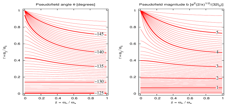
Figure 1: Contour plot showing the angle $\theta$ (left plot) and the magnitude $b$ (right plot) of the pseudomagnetic field $\boldsymbol{b}$ as a function of quantum dot anisotropy $r=\omega_{y}/\omega_{x}$ and (actual) magnetic field $z=\omega_{c}/\omega_{x}$. The angle $\theta$ is measured from the positive $x$ axis and $\boldsymbol{b}$ lies in the $x$-$z$ plane. Angles are measured in degrees and magnitudes in units of $e^{2}\sqrt{2/\pi}/(32\ell_{0})$. Shown are lines of constant $\theta$ and $b$ respectively.

The larger values of $r$ are the physically relevant ones. (The isotropic case, $\omega_{x}=\omega_{y}$ corresponds to $r=1$, whereas $r=0$ is the one-dimensional limit.) The figure shows that at a fixed magnetic field $z$, a range of pseudofield directions are available for qubit rotations by varying the voltage-tuned anisotropy $r$. In both extremes, $r=0,1$, Fig. 1 shows no dependence on $\theta$ with magnetic field $z$; in both cases, the system essentially has only one tunable parameter which, in the logical qubit space, tunes the magnitude of the pseudofield (through the hybrid magnetic length $\ell_{0}$). Figure 1 also shows how the magnitude (in units of $e^{2}\sqrt{2/\pi}/(32\ell_{0})$) of the pseudofield changes as a function of $r$ and $z$. In general, both the magnitude and direction of the pseudofield are altered by the anisotropy.

VI Explicit qubit flip sequence

By tuning $r(t)$ in real time, a qubit flip $|0\rangle\rightarrow|1\rangle$ can be performed; we give here an explicit example. It is useful to rotate our qubit, Eq. (12), so that it is oriented parallel (and antiparallel) to the direction of the pseudofield for $r=1$, given explicitly by

$$\boldsymbol{b}_{0}=\frac{-\sqrt{\pi}}{512}\left(\frac{57}{\sqrt{3}},0,21\right)\frac{e^{2}}{\ell_{0}}.$$ (14)

Thus, our rotated qubit states are $|\tilde{0}\rangle=c_{-}|0\rangle-c_{+}|1\rangle$ and $|\tilde{1}\rangle=c_{+}|0\rangle+c_{-}|1\rangle$, where $c_{\pm}=\sqrt{(b_{0}\pm b_{0z})/(2b_{0})}$.

The initial ($t=0$) qubit state is along the pseudofield direction $\boldsymbol{b}_{0}$ given by $r_{0}=1$, which, in our rotated frame, we take to lie along the $z$ axis. The field is then pulsed opt to a new value $\boldsymbol{b}_{1}$ given by, $r_{1}<1$. (This field lies in the $x$-$z$ plane.) The qubit will precess about $\boldsymbol{b}_{1}$ with period $T_{1}=\pi\hbar/b_{1}$. Half a period later, at $t=T_{1}/2$, the qubit is again in the $x$-$z$ plane, whereupon the field is pulsed back to $\boldsymbol{b}_{0}$. The qubit precess about this new field with period $T_{0}=\pi\hbar/b_{0}$. Half a period later, at $t=(T_{1}+T_{0})/2$, the field is again pulsed to $\boldsymbol{b_{1}}$ and the process is repeated every half period. (Actually, the pseudofield does not need to be switched every half period; an odd number of half-periods suffices.) If the angle $\mu$ between $\boldsymbol{b}_{0}$ and $\boldsymbol{b}_{1}$ is chosen such that $\mu=\pi/(2k)$, where $k$ is an integer, the qubit may be flipped by $k$ pulses at $\boldsymbol{b}_{1}$ with pulse width $T_{1}/2$, each separated by an interval $T_{0}/2$ at $\boldsymbol{b}_{0}$. The total switching time is $t^{\text{flip}}_{k}=kT_{1}/2+(k-1)T_{0}/2$ and can be very fast. (See below). The qubit can in fact cover the Bloch sphere by judicious choice of pseudofields, which are entirely controlled by the quantum dot anisotropy.

For definiteness, we give here numerical estimates based on material parameters for GaAs. We take $\omega_{x}=6$ meV, while $\omega_{y}$ switches between 3 and 6 meV. We also take a (fixed, uniform) magnetic field of $B=0.42$ T. Thus, $r=1,\ 0.5$ and $z=0.12$ for GaAs. For $r=1$, the pseudofield is explicitly given by Eq. (14) and yields a magnitude of $b_{0}\approx 1.61$ meV. At $r=0.5$ the magnitude is decreased, $b_{1}\approx 0.94$ meV, whereas the direction $\theta$ is increased. Figure 2 shows both the direction and magnitude of the pseudofield for these particular parameters.

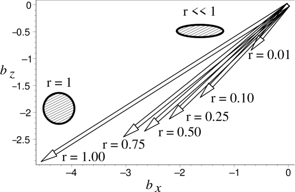
Figure 2: Direction and magnitude of magnetic field ($b_{y}=0$) for various anisotropy values $r=\omega_{y}/\omega_{x}$ at fixed magnetic field $\omega_{c}=0.12\omega_{x}$. This is essentially a plot of Eq. (13) in units of $e^{2}\sqrt{2/\pi}/(32\ell_{0})$. The hatched circle and ellipse are schematics of the quantum-dot shape at different anisotropies.

The field $\boldsymbol{b}_{1}$ is tilted away from $\boldsymbol{b}_{0}$ by $\mu=9^{\circ}$. This gives a qubit flip in ten pulses. With these pseudofield values, the precession periods are $T_{0}=1.3$ ps for $\boldsymbol{b}_{0}$ and $T_{1}=2.2$ ps for $\boldsymbol{b}_{1}$. The lower bound on the flipping time $t^{\text{flip}}$ is for a pseudofield switch every half-period; this yields $t^{\text{flip}}\approx 16.8$ ps. These times are closer to optical frequencies than what is currently achievable using pulse generators. Recent pulsed-gate experiments Fujisawa et al. (2003) employed electrical pulse-widths on the order of 10 ns. With such pulse generators, we have $t^{\text{flip}}\approx 190$ ns.

VII Discussion

Our qubit, Eq. (12), has been constructed from a linear combination of single-determinant (Hartree-Fock) state vectors, where the orbital degrees of freedom have been frozen out. But the general scheme is certainly not limited to our specific state vectors. In general, each logical qubit state can be written as a correlated many-body state $|Q\rangle=\sum_{i}\alpha^{(Q)}_{i}|\psi\rangle_{i}$, where $|Q\rangle=|0\rangle,|1\rangle$ is the logical qubit state and the $|\psi\rangle$ are antisymmetrised orthonormal states, $|\psi\rangle=|m_{1}n_{1}\sigma_{1},m_{2}n_{2}\sigma_{2},m_{3}n_{3}\sigma_{3}\rangle$, such that $|Q\rangle$ is a spin eigenstate with $S=1/2,\ S_{z}=-1/2$. Equation (12), for example, has $(m_{1}n_{1},m_{2}n_{2},m_{3}n_{3})=(00,10,20)$ for both $|Q\rangle=|0\rangle$, and $|Q\rangle=|1\rangle$; the differences between the two logical states are, in this case, solely due to spin flips and phase factors of $\pm 1$. Although there is no requirement that the orbital degrees of freedom are identical for each qubit state, it is nevertheless advantageous to have the orbital quantum numbers identical since this will reduce the electromagnetic fluctuations which would be present if the qubit rotation involved orbital transitions as well as spin transitions.

It is always possible to define the logical qubit states in such a way that they differ only by spin flips and relative phases and not by their orbital quantum numbers. This statement is not restricted to the simple (yet relevant) case of that described by Eq. (12). It is an exact result, valid even for correlated states involving many Slater determinants. Thus, voltage fluctuations due to orbital transitions can be mitigated.

It is also possible to choose the qubit states such that one is the ground spin-1/2 state and, consequently, state preparation can be a matter of equilibration.

Finally, the two qubit states will not be energetically degenerate. Thus, each qubit state will have different transport characteristics; the magnitude of current through the dot will depend differently on gate and bias voltages for each of the qubit states. This may be exploited to be used as a detection scheme for final readout.

*

Appendix A Exchange energies

The pseudofield, Eq. (13), is determined by various exchange energies. These $V_{ijkl}$ are in turn determined from the exact expression of Eq. (9) with the subscripts $(i,j,k,l)=(m_{1},m_{2},m_{3},m_{4})$ and all $n_{i}=0$. For the cases on interest here, the relevant $V_{ijkl}$ are given by:

$$V_{0110}=CX_{2},\quad\quad V_{0220}=\frac{1}{4}CX_{4},$$ (15a)

$$V_{1221}=\frac{1}{2}C\left(\frac{1}{4}X_{6}-2X_{4}+4X_{2}\right),$$ (15b)

where $C=e^{2}/(4\pi\ell_{0})$ is the Coulomb energy scale, $X_{s}=2^{(s+3)/2}\Gamma\bigl{(}(s+1)/2\bigr{)}I_{s}$, and

$$I_{s}=\int_{0}^{1}\!du\,\frac{(cu^{2}+d)^{s/2}}{(1-u^{2})^{1/2}(au^{2}+b)^{(s+1)/2}}.$$ (16)

Each $I_{s}$ is a linear combination of complete elliptic integrals of the first and second kindell

$$I_{s}=A_{s}K(m)+B_{s}E(m),$$ (17)

where $m=(\alpha_{+}^{2}-\alpha_{-}^{2})/\alpha_{+}^{2}$, and the coefficients $A_{s}$ and $B_{s}$ are given by

$$A_{2} =\frac{c}{a\sqrt{b}},$$ (18a)

$$A_{4} =\frac{1}{a^{2}\sqrt{b}}\left(c^{2}-\frac{\nu^{2}}{3b(a+b)}\right),$$ (18b)

$$A_{6} =\frac{1}{a^{3}\sqrt{b}}\left(c^{3}-\frac{c\nu^{2}}{b(a+b)}-\frac{4\nu^{3}(a+2b)}{15b^{2}(a+b)^{2}}\right),$$ (18c)

$$B_{2} =\frac{\nu}{a\sqrt{b}(a+b)},$$ (18d)

$$B_{4} =\frac{2\nu}{a^{2}\sqrt{b}(a+b)}\left(c+\frac{\nu(a+2b)}{3b(a+b)}\right),$$ (18e)

$$B_{6} =\frac{1}{a^{3}\sqrt{b}}\left(\frac{3c^{2}\nu}{a+b}+\frac{2c\nu^{2}(a+2b)}{b(a+b)^{2}}\right.$$

$$\left.\quad\quad\quad\quad\quad\quad+\frac{8\nu^{3}(a+2b)^{2}}{15b^{2}(a+b)^{3}}-\frac{3\nu^{3}}{5b(a+b)^{2}}\right),$$ (18f)

where

$$a =\beta^{2}_{+}\left(\frac{1}{\alpha^{2}_{+}}-\frac{1}{\alpha^{2}_{-}}\right)+\beta^{2}_{-}(\alpha^{2}_{-}-\alpha^{2}_{+}),$$ (19a)

$$b =\beta^{2}_{+}/\alpha^{2}_{-}+\alpha^{2}_{+}\beta^{2}_{-},$$ (19b)

$$c =\alpha^{2}_{-}\beta^{2}_{-}-\beta^{2}_{+}/\alpha^{2}_{-},$$ (19c)

$$d =\beta^{2}_{+}/\alpha^{2}_{-},$$ (19d)

$$\nu =ad-bc,$$ (19e)

and the $\alpha_{\pm}$ and $\beta_{\pm}$ are given in Eq. (4).

References

- Loss and DiVincenzo (1998) D. Loss and D. P. DiVincenzo, Phys. Rev. A 57, 120 (1998), eprint cond-mat/9701055.
- Burkard et al. (1999) G. Burkard, D. Loss, and D. P. DiVincenzo, Phys. Rev. B 59, 2070 (1999), eprint cond-mat/9808026.
- Bacon et al. (2000) D. Bacon, J. Kempe, D. A. Lidar, and K. B. Whaley, Phys. Rev. Lett. 85, 1758 (2000).
- Kempe et al. (2001) J. Kempe, D. Bacon, D. A. Lidar, and K. B. Whaley, Phys. Rev. A 63, 042307 (2001).
- Divincenzo et al. (2000) D. P. Divincenzo, D. Bacon, J. Kempe, G. Burkard, and K. B. Whaley, Nature 408, 339 (2000).
- (6) In the istropic limit of a circular quantum dot, we find and ; only the magnitude, not the direction, of the pseudofield can be changed; the direction of the pseudofield can only be changed through control of the anisotropy.
- Kyriakidis et al. (2002) J. Kyriakidis, M. Pioro-Ladriere, M. Ciorga, A. S. Sachrajda, and P. Hawrylak, Phys. Rev. B 66, 035320 (2002).
- Madhav and Chakraborty (1994) A. V. Madhav and T. Chakraborty, Phys. Rev. B 49, 8163 (1994).
- (9) Without loss of generality, we restrict in what follows.
- Jacak et al. (1997) L. Jacak, P. Hawrylak, and A. Wójs, Quantum Dots (Springer, Berlin, 1997).
- (11) The notation denotes unsymmetrised states, while denotes properly antisymmetrised and normalised states.
- (12) A smoother pulse shape for , while more realistic, would entail a careful treatment of time-ordering and would unnecessarily obfuscate the present simple example.
- Fujisawa et al. (2003) T. Fujisawa, D. G. Austing, Y. Tokura, Y. Hirayama, and S. Tarucha, J. Phys.: Condens. Matter 15, R1395 (2003).
-
(14)
We define elliptic integrals of the first and second kind as
and
respectively.