Photons and electrons as emergent phenomena

Abstract

Recent advances in condensed matter theory have revealed that new and exotic phases of matter can exist in spin models (or more precisely, local bosonic models) via a simple physical mechanism, known as ”string-net condensation.” These new phases of matter have the unusual property that their collective excitations are gauge bosons and fermions. In some cases, the collective excitations can behave just like the photons, electrons, gluons, and quarks in our vacuum. This suggests that photons, electrons, and other elementary particles may have a unified origin – string-net condensation in our vacuum. In addition, the string-net picture indicates how to make artificial photons, artificial electrons, and artificial quarks and gluons in condensed matter systems.

I Introduction

Throughout history, people have attempted to understand the universe by dividing matter into smaller and smaller pieces. This approach has proven extremely fruitful: successively smaller distance scales have revealed successively simpler and more fundamental structures. At the turn of the century, chemists discovered that all matter was formed out of a few dozen different kinds of particles – atoms. Later, it was realized that atoms themselves were composed out of even smaller particles – electrons, protons and neutrons. Today, the most fundamental particles known are photons, electrons, quarks and a few other particles. These particles are described by a field theory known as the $U(1)\times SU(2)\times SU(3)$ standard model For a review, see Cheng and Li (1991).

It is natural to wonder – are photons, electrons, and quarks truly elementary? Or are they composed out of even smaller and more fundamental objects (perhaps superstrings Green et al. (1988))? A great deal of research has been devoted to answering these questions.

However, the questions themselves may be fundamentally flawed. They are based on the implicit assumption that we can understand the nature of particles by dividing them into smaller pieces. But does this line of thinking necessarily make sense? There are many examples from condensed matter physics indicating that sometimes, this line of thinking does not make sense.

Consider, for example, a crystal. We know that a sound wave can propagate inside a crystal (see Fig. 1). According to quantum theory, these waves behave like particles called phonons. Phonons are no less particle-like than photons. But no one attempts to gain a deeper understanding of phonons by dividing them into smaller pieces. This is because phonons – as sound waves – are collective motions of the atoms that form the crystal. When we examine phonons at short distances, we do not find small pieces that make up a phonon. We simply see the atoms in the crystal.

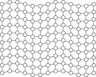
Figure 1: Sound waves in a crystal are particles called phonons, according to quantum theory.

This example suggests an alternate line of inquiry. Are photons, electrons, and other elementary particles collective modes of some deeper structure? If so, what is this “deeper structure”?

Ultimately, these questions will have to be answered by experiment. However, in this paper we would like to address the plausibility of this condensed matter model of the universe on theoretical grounds.

The laws of physics seem to be composed out of five fundamental ingredients:

1. Identical particles

2. Gauge interactions

3. Fermi statistics

4. Chiral fermions

5. Gravity

The question is whether one can find a “deeper structure” that gives rise to all five of these phenomena. In addition to being consistent with our current understanding of the universe, such a structure would be quite appealing from a theoretical point of view: it would unify and explain the origin of these seemingly mysterious and disconnected phenomena.

The $U(1)\times SU(2)\times SU(3)$ standard model fails to provide such a complete story for even the first four phenomena. Although it describes identical particles, gauge interactions, Fermi statistics and chiral fermions in a single theory, each of these components are introduced independently and by hand. For example, field theory is introduced to explain identical particles, vector gauge fields are introduced to describe gauge interactions Yang and Mills (1954) and anticommuting fields are introduced to explain Fermi statistics. One wonders – where do these mysterious gauge symmetries and anticommuting fields come from? Why does nature choose such peculiar things as fermions and gauge bosons to describe itself? We hope that the “deeper structure” that we are looking for can resolve these mysteries.

So far we do not know any structure that gives rise to, and unifies all five phenomena. In this paper, we will describe a partial solution – a structure that naturally gives rise to, and unifies the first three phenomena (and possibly also the fifth Smolin (2002)). In the language of condensed matter physics, this structure has the unusual property that its collective modes are gauge bosons (such as photons) and fermions (such as electrons).

II Locality principle

What kinds of “structures” should we look for in order to understand the origin of gauge bosons and fermions? In this paper, we will consider a very general class of structures. In fact, we will impose only one constraint on the structures we consider: locality. We will require that (a) the total Hilbert space is a product of small Hilbert spaces that describe local degrees of freedom, and that (b) the Hamiltonian only involves local interactions. For the sake of concreteness, we will also restrict our attention to lattice models.

These two requirements naturally lead us to large class of structures that we call “local bosonic models” or (generalized) “spin models”. These are lattice models where each lattice site can be in a few states $|a\rangle$ labeled by $a=0,1,2,...,N$.

The question is – can we find a local bosonic model whose collective modes are fermions and gauge bosons?

III From new phases of matter to a unification of gauge interactions and Fermi statistics

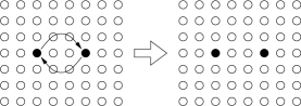
Figure 2: The empty circles correspond to sites in the $|0\rangle$ state. The solid circles correspond to sites in the $|1\rangle$ state. The states before and after the exchange are naturally the same, and hence the $|1\rangle$ states represent bosonic particles.

At first, it appears that the local bosonic models do not work. Consider, for example, a local bosonic model whose ground state has $a=0$ for every lattice site. We think of this ground state as the vacuum. A particle in the vacuum corresponds to a state with $a\neq 0$ for one site, and $a=0$ for all other sites (see Fig. 2). One can easily check that these particles are identical bosons. They are a particular kind of boson – a scalar boson. They are very different from gauge bosons and they are definitely not fermions. Thus, local bosonic models with this particularly simple ground state do not have the appropriate collective modes.

But we should not give up just yet. We know that the properties of excitations depend on the properties of the ground state. If we change the ground state qualitatively, we may obtain a new phase of matter with new excitations. These new excitations may be gauge bosons or fermions.

For many years, this was thought to be impossible. This conviction was largely based on Landau’s symmetry breaking theory – a general framework for describing phases of matter Landau (1937). According to Landau theory, phases of matter are characterized by the symmetries of their ground states. The ground state symmetry directly determines the properties of the collective excitations Landau and Lifschitz (1958). Using Landau theory, one can show that the collective modes can be very different for different ground states, but that they are always scalar bosons. There is no sign of gauge bosons or fermions.

After the discovery of the fractional quantum Hall effect (Tsui et al. (1982); Laughlin (1983)), it became clear that Landau theory could not describe all possible phases of matter. Fractional quantum Hall states contain a new kind of order – topological order Wen (1995, 2004) – that is beyond Landau theory. The collective excitations of the FQH states are not scalar bosons. Instead, they have fractional statistics Arovas et al. (1984), statistics somewhere in between Bose and Fermi statistics Leinaas and Myrheim (1977); Wilczek (1982).

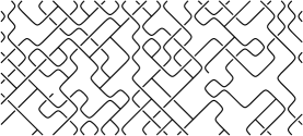
Figure 3: A typical string-net configuration in a string-net condensed state. The fluctuations of the strings correspond to gauge bosons (such as photons) and the ends of strings correspond to fermions (such as electrons).

So there is still hope. Perhaps gauge bosons and fermions can emerge from new phases of matter – phases of matter that are beyond Landau theory. This is indeed the case. Recently, it was realized that a new class of phases of matter – 3D string-net condensed phases Levin and Wen (2003); Wen (2003b); Levin and Wen (2005) – have the desired property. String-net condensed states are liquids of fluctuating networks of strings (see Fig. 3). In some sense, they are analogous to Bose condensed states, except that the condensate is formed from extended objects rather then particles. However, the collective excitations above string-net condensed states are not scalar bosons, but rather gauge bosons and fermions! Roughly speaking, the vibrations of the strings give rise to gauge bosons, while the ends of the strings correspond to fermions (see section VI).

This result may change our conception of gauge bosons and fermions. If we believe that the vacuum is some kind of string-net condensed state, then gauge bosons and fermions are just different sides of the same coin Levin and Wen (2003). In other words, string-net condensation provides a way to unify gauge bosons (such as photons) and fermions (such as electrons). It explains what gauge bosons and fermions are, where they come from, and why they exist. One application of this deeper understanding is the construction of 3D spin systems that contain both artificial photons and artificial electrons as low energy collective excitations (see section VII.2) Wen (2002, 2003b).

IV String-net condensation

What is string-net condensation? Let us first describe string-nets and string-net models. A string-net is a network of strings. The strings, which form the edges or links of the network, can come in different ”types” and can carry a sense of orientation. Thus, string-nets can be thought of as networks or graphs with oriented, labeled edges.

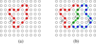
Figure 4: The empty circles are sites in the $|0\rangle$ state. The filled circles are sites in some $|a\neq 0\rangle$ state. (a) A string formed by a loop of sites with state $a$. (b) A string-net formed by a type-$a$ string, a type-$b$ string and a type-$c$ string. The string-net has two branching points where the three types of strings join.

String-net models are a special class of local bosonic models whose low energy physics is described by fluctuating string-nets. To understand how this works, consider a general local bosonic model with the states on site $\boldsymbol{i}$ labeled by $a_{\boldsymbol{i}}=0,1,...,N$. The states of this model can be thought of as configurations of string-nets in space. We regard the state with all $a_{\boldsymbol{i}}=0$ as the no-string state. We think of the state with a loop of sites in the $|a\neq 0\rangle$ state as containing a closed “type-$a$” string (see Fig. 4a). More complicated states will correspond to networks of strings as in Fig. 4b. The orientations of the corresponding strings are determined by some specified orientation convention, where one assigns some (arbitrary) orientation to each site $i$.

For most local bosonic models, this string-net picture is misleading. Each local bosonic degree of freedom fluctuates independently and the physics is better described by individual spins than by extended objects. However, for one class of local bosonic models, the string-net picture is appropriate. These are local bosonic models with the property that when strings end or change string type in empty space, the system incurs a finite energetic penalty. In these models, energetic constraints force the local bosonic degrees of freedom on the lattice sites to organize into effective extended objects. The low energy physics is then described by the fluctuations of these effective string-nets. String-net models are local bosonic models with this additional property.

Figure 5: $a$ and $a^{*}$ label strings with opposite orientations.

To specify a particular string-net model, one needs to provide several pieces of information that characterize the structure of the effective string-nets. First, one needs to give the number of string types $N$. Second, one needs to specify the branching rules – that is, what triplets of string types $(abc)$ can meet at a point. (Here for simplicity, we only consider the simplest type of branching – where three strings join at a point). The branching rules are specified by listing the “legal” branching triplets $\{(abc),(def),...\}$. For example, if $(abc)$ is legal then the string-net configuration shown in Fig. 4b is allowed. Finally, one needs to describe the string orientations: for every string type $a$, one needs to specify another string type $a^{*}$ that corresponds to a string with the opposite orientation (see Fig. 5). A string loses its sense of orientation if its string type satisfies $a=a^{*}$.

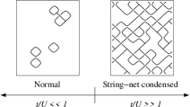
Figure 6: A schematic phase diagram for the generic string-net Hamiltonian (1). When $t/U$ is small the system is in the normal phase. The ground state consists of a few small string-nets. When $t/U$ is large the string-nets condense and large fluctuating string-nets fill all of space. We expect a phase transition between the two states at some $t/U$ of order unity. We have omitted string labels and orientations for the sake of clarity.

Given a string-net model with some string types, branching rules, and string orientations, we can imagine writing down a Hamiltonian to describe the dynamics of the string-nets. A typical string-net Hamiltonian $H$ is a sum of potential and kinetic energy pieces and a constraint term:

$$H=UH_{U}+tH_{t}+VH_{c}$$ (1)

The constraint term $H_{c}$ enforces the branching roles by making “illegal” branching points cost a huge energy $V$. Because of this term, the low energy states contain only “legal” branchings. The kinetic energy $H_{t}$ gives dynamics to these low energy string-net states while the potential energy $H_{U}$ is typically some kind of string tension. When $U\gg t$, the string tension dominates and we expect the ground state to be the no-string state with a few small string-nets. On the other hand, when $t\gg U$, the kinetic energy dominates, and we expect the ground state to consist of many fluctuating string-nets (see Fig. 6). Large string-nets with a typical length on the order of the system size fill all of space. We expect that there is a quantum phase transition between the two states at some $t/U$ on the order of unity. Because of the analogy with particle condensation, we say that the large $t$, highly fluctuating string-net phase is “string-net condensed.”

V Wave functions for string-net condensates

String-net condensed phases are new phases of matter with many interesting properties (Wen (2003a); Freedman et al. (2003); Levin and Wen (2005)). But how can we describe them quantitatively? One approach is to write down a ground state string-net wave function $\Phi(\text{string-nets})$. However, string-net condensed wave functions are usually too complicated to write down explicitly. Therefore, we will use a more indirect approach: we will describe a series of local constraint equations on string-net wave functions which have a unique solution $\Phi$. In this way, we can construct potentially complicated string-net wave functions without writing them down explicitly.

Before we state the constraint equations, we note that we can project a three-dimensional string-net configuration onto a two dimensional plane, resulting in a two-dimensional graph with branching and crossings (see Fig. 3). Thus, a wave function of three-dimensional string-nets can also be viewed as a wave function of the projected two-dimensional graphs.

The local constraints relate the amplitudes of string-net configurations that only differ by small local transformations. To write down a set of these local constraint equations or local rules, one first chooses a real tensor $d_{i}$ and two complex tensors $F^{ijm}_{kln}$, $\omega^{k}_{ij}$ where the indices $i,j,k,l,m,n$ run over the different string types $0,1,...N$. The local rules are then given by:

$$\Phi\begin{pmatrix}\includegraphics[height=21.68121pt]{Xi0.eps}\end{pmatrix} =\Phi\begin{pmatrix}\includegraphics[height=21.68121pt]{Xis0.eps}\end{pmatrix}$$

$$\Phi\begin{pmatrix}\includegraphics[scale={0.35}]{Xil0.eps}\end{pmatrix} =d_{i}\Phi\begin{pmatrix}\includegraphics[scale={0.35}]{X0.eps}\end{pmatrix}$$

$$\Phi\begin{pmatrix}\includegraphics[scale={0.35}]{XikljO.eps}\end{pmatrix} =\delta_{ij}\Phi\begin{pmatrix}\includegraphics[scale={0.35}]{XikliO.eps}\end{pmatrix}$$

$$\Phi\begin{pmatrix}\includegraphics[scale={0.35}]{XijklmXO.eps}\end{pmatrix} =\sum_{n=0}^{N}F^{ijm}_{kln}\Phi\begin{pmatrix}\includegraphics[scale={0.35}]{XijklnXO.eps}\end{pmatrix}$$

$$\Phi\begin{pmatrix}\includegraphics[scale={0.35}]{Brd1O.eps}\end{pmatrix} =\sum_{k=0}^{N}\omega^{k}_{ij}\Phi\begin{pmatrix}\includegraphics[scale={0.35}]{Brd2O.eps}\end{pmatrix}$$

$$\Phi\begin{pmatrix}\includegraphics[scale={0.35}]{Brd1pO.eps}\end{pmatrix} =\sum_{k=0}^{N}\omega^{k}_{ij}\Phi\begin{pmatrix}\includegraphics[scale={0.35}]{Brd2O.eps}\end{pmatrix}$$ (2)

where the shaded gray areas represent other parts of string-nets that are not changed. Here, the type-$0$ string is interpreted as the no-string state. We would like to mention that we have drawn the first local rule somewhat schematically. The more precise statement of this rule is that any two string-net configurations that can be continuously deformed into each other have the same amplitude. In other words, the string-net wave function $\Phi$ only depends on the topologies of the projected graphs; it only depends on how the strings are connected and crossed (see Fig. 7).

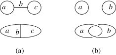
Figure 7: (a) Three strings with different connections. (b) Two strings with different crossings. The numbers of the crossings are 0 and 2 respectively.

By applying the local rules in (V) multiple times, one can compute the amplitude of any string-net configuration in terms of the amplitude of the no-string configuration. Thus (V) determines the string-net wave function $\Phi$.

However, an arbitrary choice of $(d_{i},F^{ijk}_{lmn},\omega^{k}_{ij})$ does not lead to a well defined $\Phi$. This is because two string-net configurations may be related by more then one sequence of local rules. We need to choose the $(d_{i},F^{ijk}_{lmn},\omega^{k}_{ij})$ carefully so that different sequences of local rules produce the same results. That is, we need to choose $(d_{i},F^{ijk}_{lmn},\omega^{k}_{ij})$ so that the rules are self-consistent. Finding these special tensors is the subject of tensor category theory Turaev (1994). It has been shown that only those that satisfy Levin and Wen (2005)

$$F^{ijk}_{j^{*}i^{*}0} =\frac{v_{k}}{v_{i}v_{j}}\delta_{ijk}$$

$$F^{ijm}_{kln}=F^{lkm^{*}}_{jin} =F^{jim}_{lkn^{*}}=F^{imj}_{k^{*}nl}\frac{v_{m}v_{n}}{v_{j}v_{l}}$$

$$\sum_{n=0}^{N}F^{mlq}_{kp^{*}n}F^{jip}_{mns^{*}}F^{js^{*}n}_{lkr^{*}} =F^{jip}_{q^{*}kr^{*}}F^{riq^{*}}_{mls^{*}}$$

$$\omega^{m}_{js}F^{sl^{*}i}_{kjm^{*}}\omega^{l}_{si}\frac{v_{j}v_{s}}{v_{m}} =\sum_{n=0}^{N}F^{ji^{*}k}_{s^{*}nl^{*}}\omega^{n}_{sk}F^{jl^{*}n}_{ksm^{*}}$$

$$\omega^{j}_{is} =\sum_{k=0}^{N}\omega^{k}_{si^{*}}F^{i^{*}s^{*}k}_{isj*}$$ (3)

will result in self-consistent rules and a well defined string-net wave function $\Phi$. Such a wave function describes a string-net condensed state. Here, we have introduced some new notation: $v_{i}$ is defined by $v_{i}=v_{i^{*}}=\sqrt{d_{i}}$ while $\delta_{ijk}$ is given by

$$\delta_{ijk}=\begin{cases}1,&\text{if $(ijk)$ is legal,}\\ 0,&\text{otherwise}\end{cases}$$

There is a one-to-one correspondence between 3D string-net condensed phases and solutions of (V). It is interesting to compare this with a more familiar classification scheme: the classification of crystals. In a crystal, atoms organize themselves into a very regular pattern – a lattice. Since different lattice structures are distinguished by their symmetries, we can use group theory to classify all the 230 crystals in three dimensions. In much the same way, string-net condensed states are highly structured. The different possible structures are described by solutions to (V). Tensor category theory provides a classification of the solutions of (V), which leads to a classification of string-net condensates. Thus tensor category theory is the underlying mathematical framework for understanding string-net condensed phases, just as group theory is for symmetry breaking phases.

VI Properties of collective excitations above string-net condensed states

Both crystals and string-net condensed states contain highly organized patterns. Fluctuations of these patterns lead to collective excitations. We know that the fluctuations of the lattice pattern are phonons. But what are the fluctuations of the pattern of string-net condensation? It turns out that the collective excitations above string-net condensed states are gauge bosons (Kogut and Susskind (1975); Banks et al. (1977); Foerster (1979); Foerster et al. (1980); Sakita (1980)) and fermions Levin and Wen (2003). The gauge bosons correspond to vibrations of the string-nets while the fermions correspond to the ends of strings.

Physically, the vibrating-string picture of gauge boson makes a lot of sense. We know that atoms in a crystal can vibrate in three directions and that this leads to three phonon modes. In contrast, strings can only vibrate in two transverse directions (see Fig. 8). So string vibrations can only produce excitations with two modes. This explains why gauge bosons (such as photons) have only two transverse polarizations.

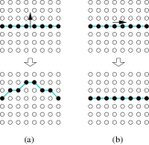
Figure 8: (a) A transverse motion of a string results in a new state and leads to a collective excitation. (b) A motion along the string does not result in any new states. Such a motion does not lead to any collective excitations.

There are many different gauge theories, each associated with a different gauge group and a different kind of gauge boson. (For example, the gauge group for electromagnetism is $U(1)$). Hence, it is natural to wonder – what is the gauge group associated with each string-net condensate? It turns out that the gauge group is determined by the same data $(d_{i},F^{ijk}_{lmn},\omega^{k}_{ij})$ that characterizes the condensate.

Given a gauge group $G$, the corresponding string types, branching rules and $(d_{i},F^{ijk}_{lmn},\omega^{k}_{ij})$ are determined as follows. The number of string types $N+1$ is given by the number of irreducible representations of $G$; each string type $i$ corresponds to a representation. The branching rules are the Clebsch-Gordan rules for $G$; that is, $(abc)$ is a “legal” branching if and only if the tensor product of the corresponding representations $a$, $b$, $c$ contains the trivial representation. The $d_{i}$ are the dimensions of the irreducible representations $i$ and the tensor $F^{ijk}_{lmn}$ is the $6j$ symbol of the group $G$. Finally, the tensor $\omega^{k}_{ij}$ is given by $\omega^{k}_{ij}=-\frac{v_{k}}{v_{i}v_{j}}$ if $i=j$ and the invariant tensor in the tensor product $i\otimes i\otimes k^{*}$ is antisymmetric, and $\omega^{k}_{ij}=\frac{v_{k}}{v_{i}v_{j}}$ otherwise. For any group $G$, this construction provides a solution $(d_{i},F^{ijk}_{lmn},\omega^{k}_{ij})$ to (V). Therefore, string-net condensed states can generate gauge bosons with any gauge group.

The second type of excitation of string-net condensed states are point defects in the condensate. These can be created by adding an open string to the condensate: new defects are formed at the ends of the string.

These defects behave like independent particles even though they are the endpoints of open strings. This is because the string connecting the two ends blends in with the condensed string already in the ground state and hence is unobservable (see Fig. 9). Only the endpoints of the string stand out and are observable. Thus the ends of strings behave like point-like objects and can be treated as particles.

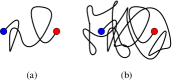
Figure 9: (a) An open string with two ends. (b) The same open string is unobservable when placed in a background of string-net condensed state. Thus the ends of open strings behave like independent particles.

It turns out that the string endpoints interact with the string vibrations just like charges interact with gauge bosons. Thus the endpoints of open strings are the charges of the gauge theory. For example, if the vibrations of the strings behave like photons, then the endpoints of the strings behave like electric charges.

For some string-net condensates the ends are bosons while for others the ends are fermions. What determines the statistics of the charges? It turns out that the statistics are also determined by the $(d_{i},F^{ijk}_{lmn},\omega^{k}_{ij})$ associated with the condensate. To see this, we note that $\Phi\begin{pmatrix}\includegraphics[scale={0.3}]{2phex.eps}\end{pmatrix}$ is the amplitude to create two pairs of particle-hole, then exchange the particles, and then annihilate the particle-hole pairs. So the phase of the exchange is the phase of $\Phi\begin{pmatrix}\includegraphics[scale={0.3}]{2phex.eps}\end{pmatrix}$ which turns out to be $e^{i\theta}=\omega^{0}_{i^{*}i}d_{i}$. Thus the end of a type-$i$ string is a fermion if $\omega^{0}_{i^{*}i}d_{i}=-1$ and a boson if $\omega^{0}_{i^{*}i}d_{i}=1$. We note that there is no way to create a single end of a string all by itself. Thus the string-net picture of fermions explains why we cannot create a single fermion.

VII Simple examples of string-net condensed states

VII.1 $Z_{2}$ gauge theory

The simplest string-net model contains only one type of string ($N=1$), and has no branching. In this case, one finds that (V) has two solutions. Each solution corresponds to a set of self-consistent local rules. The two sets of local rules, labeled by $\eta=\pm 1$, are given by

$$\Phi\begin{pmatrix}\includegraphics[height=12.28577pt]{Xl.eps}\end{pmatrix} =\Phi\begin{pmatrix}\includegraphics[height=12.28577pt]{X0.eps}\end{pmatrix},\ \ \ \ \ \Phi\begin{pmatrix}\includegraphics[height=12.28577pt]{XijklX.eps}\end{pmatrix}=\Phi\begin{pmatrix}\includegraphics[height=12.28577pt]{XijX.eps}\end{pmatrix},$$

$$\Phi\begin{pmatrix}\includegraphics[height=12.28577pt]{Brd1Z2.eps}\end{pmatrix} =\Phi\begin{pmatrix}\includegraphics[height=12.28577pt]{Brd1pZ2.eps}\end{pmatrix}=\eta\Phi\begin{pmatrix}\includegraphics[height=12.28577pt]{Brd2Z2.eps}\end{pmatrix}.$$ (4)

The local rules are so simple that we can calculate the corresponding string-net wave function explicitly. We find $\Phi(X)=\eta^{X_{c}}$, where $X_{c}$ is the number of the crossings in the string-net configuration $X$ (see Fig. 7b). The two string-net wave functions correspond to two different string-net condensed phases. In the $\eta=+1$ phase, the string fluctuations above the condensate are described by a $Z_{2}$ gauge theory. The ends of the strings are bosonic $Z_{2}$ gauge charges. In the $\eta=-1$ phase, the string fluctuations are still described by a $Z_{2}$ gauge theory, but the ends of the strings are fermions.

VII.2 $U(1)$ gauge theory with fermions

To construct a string-net condensate with photon-like and electron-like excitations, we need a string-net model with oriented stings labeled by integers $a=0,\pm 1,\pm 2,...$. We need the following branching rules: $(abc)$ is legal if $a+b+c=0$ (see Fig. 10). These branching rules have a simple physical interpretation if we view the strings as electric flux lines and the labels $a$ as measuring the amount of electric flux flowing through the string. The branching rule $a+b+c=0$ is then simply a statement of flux conservation (e.g. Gauss’ law).

Figure 10: The branching rule $a+b+c=0$.

One finds that (V) has two solutions. One of these solutions can be represented by the following local rules:

$$\Phi\begin{pmatrix}\includegraphics[scale={0.35}]{XijklmXU1.eps}\end{pmatrix} =\Phi\begin{pmatrix}\includegraphics[scale={0.35}]{XijklnXU1.eps}\end{pmatrix},$$

$$\Phi\begin{pmatrix}\includegraphics[scale={0.35}]{Brd1O.eps}\end{pmatrix} =\Phi\begin{pmatrix}\includegraphics[scale={0.35}]{Brd1pO.eps}\end{pmatrix}$$

$$=(-1)^{i\times j}\Phi\begin{pmatrix}\includegraphics[scale={0.35}]{Brd2U1.eps}\end{pmatrix}.$$

The local rules lead to the string-net wave function $\Phi(X)=(-1)^{X_{co}}$, where $X_{co}$ is the number of the crossings between strings labeled by odd integers, in the string-net configuration $X$.

The collective excitations in the above string-net condensed phase are $U(1)$ gauge bosons which behave in every way like the photons in our vacuum. We call these excitations “artificial photons.” The ends of type-$1$ strings behave like fermions with unit charge. They interact with artificial photons in the same way that electrons interact with photons. Therefore, we call the ends of type-$1$ strings “artificial electrons.” More generally, the ends of type-$i$ strings behave like bound states of $i$ artificial electrons.

VIII Artificial photons and Artificial electrons

We have seen that, for any solution $(d_{i},F^{ijk}_{lmn},\omega^{ik}_{j})$ of (V), we can construct a corresponding string-net condensed state. The properties of collective excitations of this state are determined by the data $(d_{i},F^{ijk}_{lmn},\omega^{ik}_{j})$. Now the question is, can we realize such a string-net condensed state in a condensed matter system? The answer is yes, at least theoretically. It was shown recently that for every solution $(d_{i},F^{ijk}_{lmn},\omega^{ik}_{j})$ of (V), we can construct an exactly soluble local bosonic model such that the ground state of the model is the corresponding string-net condensed state Levin and Wen (2005). The collective excitations in such a model are the gauge bosons and fermions discussed above. So in principle, we can construct condensed matter systems which can generate gauge bosons with arbitrary gauge groups and fermions with arbitrary gauge charges.

However, these exactly soluble bosonic models are usually complicated and hard to realize in real materials. On the other hand, if we only want to make artificial photons, then there is a simple spin-$S$ model on the (three-dimensional) pyrochlore lattice. The Hamiltonian is given by

$$H=J_{1}\sum_{\boldsymbol{i}}(S^{z}_{\boldsymbol{i}})^{2}+J_{2}\sum_{\langle\boldsymbol{i}\boldsymbol{j}\rangle}S^{z}_{\boldsymbol{i}}S^{z}_{\boldsymbol{j}}+J_{\perp}\sum_{\langle\boldsymbol{i}\boldsymbol{j}\rangle,a=x,y}S^{a}_{\boldsymbol{i}}S^{a}_{\boldsymbol{j}},$$ (5)

where $\langle\boldsymbol{i}\boldsymbol{j}\rangle$ are nearest neighbors. It turns out that the above model exhibits string-net condensation for integer $S$ and $J_{1}\gg|J_{\perp}^{3}/J_{1}^{2}|\gg|J_{1}-J_{2}|$ Wen (2003a). In this limit, the model contains gapless artificial photons as its low energy excitations. The ground state – a string-net condensed state – represents a new state of matter that cannot be described by Landau’s symmetry breaking theory. A similar model with spin $S=1/2$ may also contain artificial photons Hermele et al. (2004).

To understand this result and its generalizations to other lattices, it is useful to consider the low energy behavior of (5). In the limit of large $J_{1}\approx J_{2}$, the above model has a low energy sector consisting of states satisfying $S_{t1}^{z}+S_{t2}^{z}+S_{t3}^{z}+S_{t4}^{z}=0$ for all tetrahedra $t$ in the pyrochlore lattice. Restricting to this subspace – which can be thought of as the string-net sector – we find that the low energy effective Hamiltonian is given by

$$H_{eff} =g\sum_{\boldsymbol{p}}(B_{\boldsymbol{p}}+h.c.)+\delta J\sum_{\boldsymbol{i}}(S^{z}_{\boldsymbol{i}})^{2},$$ (6)

$$B_{\boldsymbol{p}} \equiv S_{1}^{+}S_{2}^{-}S_{3}^{+}S_{4}^{-}S_{5}^{+}S_{6}^{-}.$$

Here the sum runs over the hexagonal plaquettes $\boldsymbol{p}$ of the pyrochlore lattice, and $1,\cdots,6$ label the sites of the hexagon $\boldsymbol{p}$. The two coupling constants are given by $\delta J=J_{1}-J_{2}$ and $g=\frac{3J_{\perp}^{3}}{2J_{2}^{2}}$.

According to the string picture, the $\delta J$ term corresponds to a string tension term, while the $g$-term corresponds to a string kinetic energy term. When $|g|\gg|\delta J|$, the string fluctuations overwhelm the string tension, and the string-nets condense. The result is a new state of matter with gapless artificial photons as its low energy excitations.

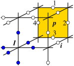
Figure 11: A picture of the cubic lattice model (7) with artificial photons. The term $Q_{\boldsymbol{I}}=(-1)^{\boldsymbol{I}}\sum_{\text{legs of }\boldsymbol{I}}S_{\boldsymbol{i}}^{z}$ acts on the six “legs” of $\boldsymbol{I}$ – that is, the six spins adjacent to $\boldsymbol{I}$, drawn above as filled dots. The term $B_{\boldsymbol{p}}=S^{+}_{1}S^{-}_{2}S^{+}_{3}S^{-}_{4}$ acts on the four spins, labeled by 1,2,3,4, along the boundary of the plaquette $\boldsymbol{p}$.

With this understanding, one can easily generalize this result to other lattices. A particularly simple example is a cubic lattice model with spins on the links Levin and Wen (2004). The Hamiltonian is given by

$$H =V\sum_{\boldsymbol{I}}Q^{2}_{\boldsymbol{I}}+g\sum_{\boldsymbol{p}}(B_{\boldsymbol{p}}+h.c.)+\delta J\sum_{\boldsymbol{i}}(S^{z}_{\boldsymbol{i}})^{2},$$ (7)

$$B_{\boldsymbol{p}} =S^{+}_{1}S^{-}_{2}S^{+}_{3}S^{-}_{4},\ \ \ \ \ \ \ \ \ Q_{\boldsymbol{I}}=(-1)^{\boldsymbol{I}}\sum_{\text{legs of }\boldsymbol{I}}S_{\boldsymbol{i}}^{z},$$

where $\boldsymbol{I}=(I_{x},I_{y},I_{z})$ labels the vertices, $\boldsymbol{i}$ labels the links and $\boldsymbol{p}$ labels the plaquettes of the cubic lattice (see Fig. 11). Also, $(-1)^{\boldsymbol{I}}\equiv(-1)^{I_{x}+I_{y}+I_{z}}$.

As in the previous case, the model (7) has a low energy sector consisting of string-net states, in the limit of large $V$. When $|g|\gg|\delta J|$, the string-nets condense giving rise to a phase with gapless artificial photons as its low energy excitations.

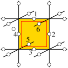
Figure 12: A picture of the modified cubic lattice model (8) with artificial photons and artificial electrons. The term $\tilde{B}_{\boldsymbol{p}}=S^{+}_{1}S^{-}_{2}S^{+}_{3}S^{-}_{4}(-1)^{S^{z}_{5}+S^{z}_{6}}$ acts on the four spins, labeled by 1,2,3,4, along the boundary of the plaquette $\boldsymbol{p}$, and the two spins, labeled by 5,6 on the “crossed” links adjacent to $\boldsymbol{p}$. The “crossed” links are defined by projecting the cubic lattice onto the plane and drawing a small closed curve just inside but along the boundary of each plaquette $\boldsymbol{p}$. The edges adjacent to $\boldsymbol{p}$ that cross this closed curve, are known as “crossed” links.

In the above two models, the electric charges are bosonic. However, one can obtain models with fermionic electric charges (e.g. artificial electrons) by modifying these Hamiltonians in a simple way: one simply multiplies the ring exchange term $B_{\boldsymbol{p}}$ by a phase factor which depends on the spins adjacent to the plaquette $\boldsymbol{p}$ Levin and Wen (2004). In the cubic lattice model (7), this factor is of the form $(-1)^{S^{z}_{5}+S^{z}_{6}}$, where $S_{5},S_{6}$ are two of the 16 spins adjacent to $\boldsymbol{p}$. The modified Hamiltonian is thus

$$H =V\sum_{\boldsymbol{I}}Q^{2}_{\boldsymbol{I}}+g\sum_{\boldsymbol{p}}(\tilde{B}_{\boldsymbol{p}}+h.c.)+\delta J\sum_{\boldsymbol{i}}(S^{z}_{\boldsymbol{i}})^{2},$$ (8)

$$\tilde{B}_{\boldsymbol{p}} =S^{+}_{1}S^{-}_{2}S^{+}_{3}S^{-}_{4}(-1)^{S^{z}_{5}+S^{z}_{6}},\ \ \ \ \ \ Q_{\boldsymbol{I}}=(-1)^{\boldsymbol{I}}\sum_{\text{legs of }\boldsymbol{I}}S_{\boldsymbol{i}}^{z}$$

The two spins $S_{5},S_{6}$ associated with each plaquette $\boldsymbol{p}$ are specified as follows: first, one projects the cubic lattice onto the plane. Then one examines the $16$ spins adjacent to each plaquette $\boldsymbol{p}$. Two of these spins will be located on links that “cross” the boundary of the plaquette $\boldsymbol{p}$ – in the sense that they cross a closed curve drawn just inside but along the boundary of $\boldsymbol{p}$. The spins $S_{5},S_{6}$ are precisely the two spins located on these “crossed” links (see Fig. 12).

The ground state of (8) exhibits a different type of string-net condensation from the previous two models. While string fluctuations still correspond to $U(1)$ gauge bosons (e.g. artificial photons), the ends of strings now correspond to charged fermions (e.g. artificial electrons).

IX Are we living in a noodle soup?

We have seen that string-net condensed states naturally give rise to gauge bosons (such as photons) and fermions (such as electrons). Thus, the existence of photons and electrons is no longer mysterious if we assume that our vacuum is a string-net condensate. Photons are vibrations of condensed strings, while electrons are the ends of the strings.

But is our vacuum really a string-net condensed state? Photons and electrons are just two of the elementary particles in nature. So the real question is – can string-net theory explain the other elementary particles? The answer is yes and no. String-net condensation naturally explains three of the mysteries of nature discussed in the introduction – identical particles, gauge interactions and Fermi statistics. But so far we do not know how to explain the fourth and the fifth mysteries – chiral fermions and gravity. In terms of elementary particles, we can construct a string-condensed local bosonic model that produces $U(1)$ gauge bosons (photons), $SU(3)$ gauge bosons (gluons), leptons (which includes electrons), and quarks Wen (2003b), but we do not know how to produce the neutrinos, $SU(2)$ gauge bosons, or gravitons.

The problem with the neutrinos and the $SU(2)$ gauge bosons is the famous chiral-fermion problem Lüscher (2001). Neutrinos are chiral fermions and the $SU(2)$ gauge bosons couple chirally to other fermions. At the moment, we do not know how to obtain chiral fermions and chiral gauge theories from any local lattice model, much less a local bosonic model.

Gravity is also a formidable problem. To obtain general relativity from a local bosonic model, one must develop a quantum theory of gravity, a notoriously difficult task. However, there is one possible approach: loop quantum gravity Smolin (2002). Remarkably, it appears that the theory of loop quantum gravity can be reformulated in terms of a particular kind of string-net, where the strings are labeled by positive integers. This means that, in addition to gauge interactions and Fermi statistics, string-net condensation in a spin model may also give rise to gravity!

X Emergence vs. reductionism

In this paper, we propose local bosonic models as a possible origin of elementary particles. But local bosonic models are far from unique. Should we be worried about being overwhelmed with possibilities? If one takes a reductionist point of view, this is indeed a serious concern. The string-net picture does not tell us how to derive a unique local bosonic model that describes our universe, and the models it does suggest are neither simple nor beautiful.

However, according to the point of view of emergence Anderson (1972) – the point of view we take in this paper – this is not an issue. We are not interested in the details of the particular model that produces the observed elementary particles. We expect that these details are both complicated and irrelevant to the low energy emergent physics we observe around us. Instead, we are interested in the general mechanism that leads to these particles. In this paper we have shown that string-net condensation may be one such mechanism. Photons and electrons will emerge if the local bosonic models are in a particular string-net condensed phase, irrespective of microscopic details.

On theoretical grounds, string-net condensation appears to be a promising approach to understanding our universe. Ultimately, however, the validity of the string-net picture, or more generally the condensed matter picture of the universe, will be decided by experiment. As we probe nature at shorter and shorter distance scales, we will either find increasing simplicity, as predicted by the reductionist particle physics paradigm, or increasing complexity, as suggested by the condensed matter point of view. We will either establish that photons and electrons are elementary particles, or we will discover that they are emergent phenomena – collective excitations of some deeper structure that we mistake for empty space.

This research is supported by NSF Grant No. DMR–01–23156, NSF-MRSEC Grant No. DMR–02–13282, and NFSC no. 10228408.

References

- Anderson (1972) Anderson, P. W., 1972, Science 177, 393.
- Arovas et al. (1984) Arovas, D., J. R. Schrieffer, and F. Wilczek, 1984, Phys. Rev. Lett. 53, 722.
- Banks et al. (1977) Banks, T., R. Myerson, and J. B. Kogut, 1977, Nucl. Phys. B 129, 493.
- For a review, see Cheng and Li (1991) Cheng, T. P., and L. F. Li, 1991, Gauge theory of elementary particle physics (Oxford Univ. Press, Oxford).
- Foerster (1979) Foerster, D., 1979, Physics Letters B 87, 87.
- Foerster et al. (1980) Foerster, D., H. B. Nielsen, and M. Ninomiya, 1980, Phys. Lett. B 94, 135.
- Freedman et al. (2003) Freedman, M., C. Nayak, K. Shtengel, K. Walker, and Z. Wang, 2003, cond-mat/0307511.
- Green et al. (1988) Green, M. B., J. H. Schwarz, and E. Witten, 1988, Superstring Theory (Cambridge University Press).
- Hermele et al. (2004) Hermele, M., M. P. A. Fisher, and L. Balents, 2004, Phys. Rev. B 69, 064404.
- Kauffman and Lins (1994) Kauffman, L., and S. Lins, 1994, Tempereley-Lieb Recoupling Theory and Invariants of 3-Manifolds (Princeton University Press, Princeton).
- Kogut and Susskind (1975) Kogut, J., and L. Susskind, 1975, Phys. Rev. D 11, 395.
- Landau (1937) Landau, L. D., 1937, Phys. Z. Sowjetunion 11, 26.
- Landau and Lifschitz (1958) Landau, L. D., and E. M. Lifschitz, 1958, Statistical Physics – Course of Theoretical Physics Vol 5 (Pergamon, London).
- Laughlin (1983) Laughlin, R. B., 1983, Phys. Rev. Lett. 50, 1395.
- Leinaas and Myrheim (1977) Leinaas, J. M., and J. Myrheim, 1977, Il Nuovo Cimento 37B, 1.
- Levin and Wen (2003) Levin, M., and X.-G. Wen, 2003, Phys. Rev. B 67, 245316.
- Levin and Wen (2004) Levin, M., and X.-G. Wen, 2004, hep-th/0507118 .
- Levin and Wen (2005) Levin, M., and X.-G. Wen, 2005, Phys. Rev. B 71, 045110.
- Lüscher (2001) Lüscher, M., 2001, hep-th/0102028 .
- Penrose (1971) Penrose, R., 1971, in Quantum Theory and Beyond, edited by T. Bastin (Cambridge Univ. Press, Cambridge).
- Sakita (1980) Sakita, B., 1980, Phys. Rev. D 21, 1067.
- Smolin (2002) Smolin, L., 2002, Three Roads to Quantum Gravity (Basic Books).
- Tsui et al. (1982) Tsui, D. C., H. L. Stormer, and A. C. Gossard, 1982, Phys. Rev. Lett. 48, 1559.
- Turaev (1994) Turaev, V. G., 1994, Quantum invariants of knots and 3-manifolds (W. de Gruyter, Berlin-New York).
- Wen (1995) Wen, X.-G., 1995, Advances in Physics 44, 405.
- Wen (2002) Wen, X.-G., 2002, Phys. Rev. Lett. 88, 11602.
- Wen (2003a) Wen, X.-G., 2003a, Phys. Rev. B 68, 115413.
- Wen (2003b) Wen, X.-G., 2003b, Phys. Rev. D 68, 065003.
- Wen (2004) Wen, X.-G., 2004, Quantum Field Theory of Many-Body Systems – From the Origin of Sound to an Origin of Light and Electrons (Oxford Univ. Press, Oxford).
- Wilczek (1982) Wilczek, F., 1982, Phys. Rev. Lett. 49, 957.
- Yang and Mills (1954) Yang, C. N., and R. L. Mills, 1954, Phys. Rev. 96, 191.