Theory of Edge States in Systems with Rashba Spin-Orbit Coupling
Abstract
We study the edge states in a two dimensional electron gas with a transverse magnetic field and Rashba spin-orbit coupling. In the bulk, the interplay between the external field perpendicular to the gas plane and the spin-orbit coupling leads to two branches of states that, within the same energy window, have different cyclotron radii. For the edge states, surface reflection generates hybrid states with the two cyclotron radii. We analyze the spectrum and spin structure of these states and present a semiclassical picture of them.
pacs:
71.70.Di,71.70.Ej,73.20-rI Introduction
Since the seminal spin-transistor proposal by Datta and Das,Datta and Das (1990) it has been recognized that the spin-orbit interaction may be a useful tool to manipulate and control the spin degree of freedom of the charge carriers. This opens novel opportunities for the developing field of spintronics.Awschalom et al. (2002) The challenging task of building spin devices based purely on semiconducting technology requires to inject, control and detect spin polarized currents without using strong magnetic fields. For this purpose, the spin-orbit coupling may be a useful intrinsic effect that links currents, spins and external fields. During the last years a number of theoretical and experimental papers were devoted to study the effect of spin-orbit coupling on the electronic and magnetotransport properties of two dimensional electron gases (2DEG).Aronov and Lyanda Geller (1993); Hirsch (1999); Molenkamp et al. (2001); Zümbuhl et al. (2002); Governale and Zülicke (2002); Streda and Seba (2003); Mishchenko and Halperin (2003); Schliemann and Loss (2003); Sinova et al. (2004); Chen et al. ; Rashba (2004) This is endorsed by the fact that, in some of the semiconducting heterostructures used to confine the electron or hole gas, the spin orbit interaction is large. Moreover it may be varied by changing carrier densities or gating with external electric fields.Nitta et al. (1997); Miller et al. (2003)
In many transport experiments in 2DEG with a transverse magnetic field, including quantum Hall effectHalperin (1982) and transverse magnetic focusing,van Houten et al. (1989); Beenakker and van Houten (1991); Potok et al. (2002) edge states play a central role. To our knowledge, a detailed analysis of the effect of the spin-orbit coupling on the edge states has not been done yet. In this paper we present a theory for edge states in 2DEG with transverse magnetic fields and a Rashba term describing the spin orbit interaction.Rashba (1960)
First we focus on the quantum mechanical solution. By numerical diagonalization of the Hamiltonian in a truncated Hilbert space we calculate the energy spectrum and the wavefunctions that, as we show below, present an intricate structure. Then we resort to a semiclassical analysis to interpret and illustrate the nature of the edge states in the high energy or low field limit.
Our starting point is a 2DEG with Rashba coupling and an external magnetic field perpendicular to the plane containing the electron gas:
| (1) |
where is the effective mass of the carriers, , with and being the -component of the momentum and vector potential respectively, is the Rashba coupling parameter, are the Pauli matrices and is the gyromagnetic factor. The last term is the lateral confining potential. For simplicity, from hereon we consider a hard wall potential that confines the electrons in the transverse -direction: for and infinite otherwise.
II The Quantum Solution
In the geometry where electrons are confined in the -direction, it is convenient to use the Landau gauge and write the wavefunction in the form:
| (2) |
with the function expanded in the basis set of the infinite potential well
| (3) |
The Schrödinger equation leads to the following equations for the spinors
| (6) | |||
| (9) |
with , and proportional to the matrix elements of the operators , and respectively,
| (11) |
Here, is the cyclotron frequency, and . We solve these equations in a truncated Hilbert space disregarding the highest energy states. Typically we take a matrix Hamiltonian of dimension of a few hundreds and keep the first thirty states. In all cases the width of the sample is taken large enough to have the cyclotron radius smaller than . The right and left edge states are then well separated in real space.
For the states are equal to the bulk states, except for exponential corrections. The wave functions and the energy spectrum reproduces the known results: in the bulk the spin-orbit coupling mixes the two spin components and there are two branches of states with energies given byRashba (1960); Bychkov and Rashba (1984)
| (12) |
with and a single state () with energy . The corresponding eigenfunctions for are
| (13) |
and
| (14) |
Here is the length of the sample in the -direction, is the harmonic oscillator wavefunction centered at the coordinate , and
| (15) |
The wavefunction of the state with is
| (16) |

In the bulk (), the ground state has the spin along the -direction. In the excited states the spin is tilted with an expectation value of its -component that decreases as and increase. The condition , that is equivalent to for all , is referred as the weak field condition.Bychkov and Rashba (1984) For large enough , when , the spin-orbit dominates and .
For high fields or low electron density, the physical properties of the system are dominated by the states with low quantum number . We first consider this case and present the results for the first few Landau levels.
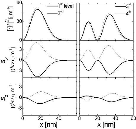
As the momentum parallel to the edge varies, the center of gravity of the wavefunctions changes and as it approaches the sample edge,the effect of the confining potential becomes important generating the -dependent dispersion of the energy levels.Halperin (1982)The interplay of the spin-orbit coupling and the confining potential produce a tilting of the spin for all the edge states. Edge states probability densities and the corresponding spin densities are shown in Fig.1 for . The spin is predominantly in the -plane even for the lowest energy edge states and the sign of the spin densities alternates as the energy increases. The current carried by these states is then polarized and for the parameters of the figure the polarization is determined by the Rashba coupling. We use the charge and spin currents operators defined as: for the charge current and and for the spin currents.Rashba (2003) In these expressions the velocity operator in the -direction is given by
| (17) | |||||
The total current densities, defined as where the sum runs over all occupied states, are shown in Fig.2 for different values of the Fermi energy. The charge and current densities are confined at the sample edge indicating that they are due to the edge states. Conversely the current density has a non-zero value inside the sample. The origin of this current can be understood in terms of the simple semiclassical picture shown in Fig.2e: electrons moving in the positive (negative) -direction have a positive (negative) projection of the spin along the -axis. Since the spin is not conserved, these currents do not necessarily produce spin accumulation in samples with constrictions or edges perpendicular to the current direction.Rashba (2004)
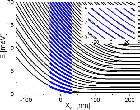
Let us now consider the low field case where many Landau levels are below the Fermi energy. The energy spectrum as a function of is presented in Fig.3. For the bulk states, the typical energy splitting of the two branches and is different (see Eq.(12)), leading to a beat in the total energy spectrum. Within the same energy interval, the two branches have different quantum number and consequently different cyclotron radius . We takeFerry and Goodnick (1997)
| (18) |
that for large gives . According to equation (12), in this limit states with approximately the same energy belonging to different branches have cyclotron radius differing in . Note that the radius difference in this large approximation does not depend on .
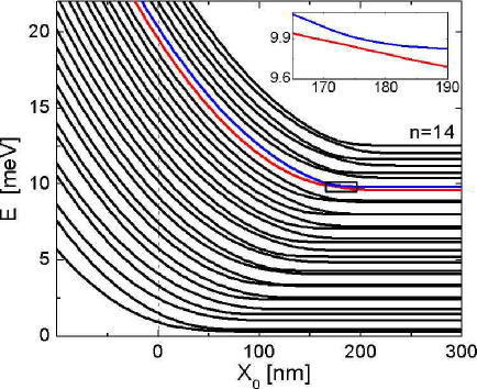
For the effect of the confining potential becomes important and the two bulk branches mix leading to edge states that combine the two cyclotron radii. This mixing is apparent from the energy spectrum that presents level anticrossings as shown in the inset of Fig.3.
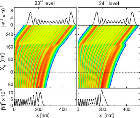
The behavior of the levels 23 and 24 is illustrated in Fig.4. In the top panel the figure their probability densities for are shown. These states correspond to a state of the branch with and a state of the branch with respectively. The branch state radius is larger than the branch one as can be inferred from the figure. We can follow the evolution of these states as changes from to a negative value. A contour plot illustrating this evolution in shown in the central panel of Fig.4. For a sudden change in the wave function spatial extension is observed. States belonging to the bulk branch shrink for due to the mixing with the branch states. Conversely, states belonging to the bulk branch expand for . This sudden change in the wave function extension is of the order of . The lower panel of Fig.4 shows the probability densities of the two levels for a negative value of .
For the number of nodes of the wavefunction of a given level is conserved as changes. With spin-orbit coupling, the anticrossing of energy levels is an indication that the wavefunctions change in character as changes. Then, for a given energy level the number of maxima of the probability density is no longer conserved as it is shown in Fig.4. It is also interesting to analyze the spin densities associated to these states.
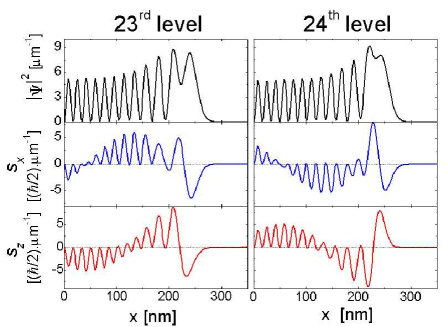
The spin structure of the edge states for is shown in Fig.5. The spin densities and show an intricate behavior due to the beating of two contributions. This is a consequence of the mixing of states that are and in character. As we discuss below the semiclassical analysis also unveils that edge states are formed by combining states with different radii and different spin projections.
III The Semiclassical Solution
III.1 Bulk States
In a recent approach,Pletyukhov et al. (2002) both the orbital and the spin degrees of freedom have been treated semiclassicaly in an extended phase space. The spin coherent state is defined as
| (19) |
where is a -number. A unit vector associated with the classical spin is defined in terms of the coherent state , which for spin reads
| (20) |
with components determined by
| (21) |
and .
The classical phase-space symbol of the Hamiltonian defined in Eq.(1) isPletyukhov et al. (2002)
| (22) |
where the first term is the classical Hamiltonian without spin orbit coupling and
| (23) |
The equations of motion are:
| (24) |
whose solutions represent the classical orbits in the extended phase space. In bulk there is an additional constant of motion besides the energy and the system is classically integrable. We are interested in the periodic solutions of Eq.(24) from which the action integral can be computed in order to apply an EBK quantization scheme.Gutzwiller (1991) We propose and replace it in Eq.(24). For the initial conditions are impossed leading to
| (25) |
where we have defined . The normalization condition for the spin components gives an algebraic equation of order fourth in that to leading order in (semiclassical limit) gives
| (26) |
Given the two frequencies one must go one step further to find an explicit expression for the cyclotron radius. Replacing Eq.(25) evaluated a in the equation for the energy conservation , and taking into account the value of obtained in (26), we find
| (27) |
Therefore for a given energy the periodic solutions result in two orbits of radii , frequencies and opposite values of the spin respectively. The cyclotron radii difference is in exact correspondence with the quantum mechanical estimate that we obtained for large . In these two orbits, with different radii and frequencies, the electron has the same velocity; that is .
Once we know the periodic solutions in extended phase space we need to compute the action integral . Following Ref.[Pletyukhov et al., 2002], the action can be expressed as:
with . The EBK quantization rule sets
| (29) |
where is an integer and is the sum of the phase shifts acquired at the turning points of the motion Gutzwiller (1991). For the bulk solutions the turning points are two caustics giving a total phase shift . Replacing Eq.(27) in Eq.(III.1) we finally obtain
| (30) |
which is the quantum spectrum for the bulk states (neglecting the zero point energy) Bychkov and Rashba (1984). With the notation we emphasize that for a given quantum index , the (energy associated to ) is lower than (energy associated to ).
III.2 Edge States
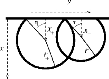
As we mentioned above, for the bulk () and () branches mix, and the wavefunctions spatial extension present a remarkable change. The avoided level crossings structure observed around in the energy spectrum is the fingerprint of this behavior. The semiclassical image that we propose consists of a skipping orbit formed by a series of translated circular arcs of radii and and centers and in the direction respectively (see Fig.6). The center coordinate of these circular arcs changes at each specular reflection. In Fig.6 this primitive orbit is plotted for a complete period of the motion. The fact that the reflection at the boundary is specular is guaranteed by the conservation of the modulus of the velocity ( ) and can be cast in the form
| (31) |
being the angle depicted in Fig.6.
As it can be inferred from the semiclassical solutions obtained in Eq.(25), to lowest order in the in plane spin components ( and ) of the orbit have opposite signs than those of the orbit and in both cases is . Therefore the spin conservation is guaranteed at each specular reflection of the skipping orbit with the boundary if and . Our goal is to perform a semiclassical quantization employing this classical skipping orbit. The semiclassical approach is fully justified for angles and we will obtain the energy spectrum and the dispersion relation quite accurately around .
We proceed analogously to the previous section, taking now into account that the orbital motion projected on the axis is periodic with a period . For the sake of clarity we divide the action integral in two terms . The action associated to the orbital motion is
| (32) | |||||
For the spin degrees of freedom the action integral is straightforward to evaluate and gives . For the skipping orbit the phase shift is , due to the fact that we have to consider now for each period of motion two bounces with the boundary and also two caustics. Replacing the obtained values for and into Eq.(III.1) we finally obtain
| (33) |
as a function of the parameter .
For , is and the energy levels are
| (34) |
To obtain the dispersion relation, we proceed numerically due to the fact that the variable depends on the energy through the cyclotron radii. In order to compare with the quantum mechanical solution for one needs to rewrite Eq.(33) as a function of the center of the classical skipping orbit which plays the role of for the edge states. For we have checked that , or leads to almost the same dispersion relation. In Fig.8 we plot Eq.(33) after chossing . Notice that the semiclassical solution follows quite satisfactory the quantum results even in the low energy region and it is almost indistinguishable from them for .
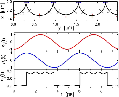
We end this section by presenting results of the numerical integration of the semiclassical equations Eq.(24) using a fourth order Runge-Kutta algorithm. The results agree with the analytical solution obtained to lowest order in , and they are summarized in Fig.8 where the skipping orbit with two radii is clearly observed. The components and of the classical vector show the expected behavior with a continuous evolution at the bouncing point. The out of plane component is small and presents fast changes at the bouncing points. This component decreases as the energy increases in agreement with the semiclassical assumption that, to lowest order in , predicts .
IV Summary and Conclusions
We have analyzed the eigenstates and the energy spectrum of a 2DEG with spin-orbit coupling in the presence of a perpendicular magnetic field. We focused on the edge states that appear when the 2DEG is confined in the transverse -direction by a square well potential. We first discussed the low energy states in the high field limit. The rest of our work was devoted to study the high energy states (high quantum number ). In this regime, the spin-orbit coupling has an important effect on the edge states: while for the the edge states with (that corresponds to ) have an energy separation ,van Houten et al. (1989) for the energy separation is , see Eq. (34). As pointed out in section II, the effect of the spin-orbit coupling increases with and with the quantum number , and there is always a high energy regime where the spin-orbit coupling dominates. In this high regime, the energy spectrum of the edge states follows Eq. (34).
In the bulk, states with large and small radii are quasi-degenerated. The bouncing at the surface mixes them leading to hybrid states that combine large and small radii. The mixing is evident in the quantum solution where the energy spectrum versus shows avoided level crossings, a fingertip of level mixing.
The spin texture of these states is also discussed in terms of the classical solution. To lowest order in the spin lies in the plane of the 2DEG and its direction is perpendicular to the velocity. The relative orientation of the spin with respect to the velocity is different along the segments with large and small cyclotron radius.
The picture obtained with the semiclassical approximation accounts for the quantum mechanical prediction of a splitted transverse focusing peaksUsaj and Balseiro (2004) that was recently experimentally observed in hole gas in GaAs.Rokhinson et al. (2004)
Partial financial support by ANPCyT Grant 99 3-6343 and Foundación Antorchas, Grants 14169/21 and 14116/192, are gratefully acknowledged.
References
- Datta and Das (1990) S. Datta and B. Das, Appl. Phys. Lett. 56, 665 (1990).
- Awschalom et al. (2002) D. Awschalom, N. Samarth, and D. Loss, eds., Semiconductor Spintronics and Quantum Computation (Springer, New York, 2002).
- Aronov and Lyanda Geller (1993) A. G. Aronov and Y. B. Lyanda–Geller, Phys. Rev. Lett. 70, 343 (1993).
- Hirsch (1999) J. E. Hirsch, Phys. Rev. Lett. 83, 1834 (1999).
- Molenkamp et al. (2001) L. W. Molenkamp, G. Schmidt, and G. E. W. Bauer, Phys. Rev. B 64, 121202 (2001).
- Zümbuhl et al. (2002) D. M. Zümbuhl, J. B. Miller, C. M. Marcus, K. Campman, and A. C. Gossard, Phys. Rev. Lett. 89, 276803 (2002).
- Governale and Zülicke (2002) M. Governale and U. Zülicke, Phys. Rev. B 66, 07331 (2002).
- Streda and Seba (2003) P. Streda and P. Seba, Phys. Rev. Lett. 90, 256601 (2003).
- Mishchenko and Halperin (2003) E. G. Mishchenko and B. I. Halperin, Phys. Rev. B 68, 045317 (2003).
- Schliemann and Loss (2003) J. Schliemann and D. Loss, Phys. Rev. B 68, 165311 (2003).
- Sinova et al. (2004) J. Sinova, D. Culcer, Q. Niu, N. A. Sinitsyn, T. Jungwirth, and A. H. MacDonald, Physical Review Letters 92, 126603 (2004).
- (12) H. Chen, J. J. Heremans, J. A. Peters, J. P. Dulka, and A. O. Govorov, eprint cond-mat/0308569.
- Rashba (2004) E. I. Rashba (2004), eprint cond-mat/0404723.
- Nitta et al. (1997) J. Nitta, T. Akazaki, H. Takayanagi, and T. Enoki, Phys. Rev. Lett. 78 (1997).
- Miller et al. (2003) J. B. Miller, D. M. Zümbuhl, C. M. Marcus, Y. B. Lyanda-Geller, D. Goldhaber-Gordon, K. Campman, and A. C. Gossard, Phys. Rev. Lett. 90, 076807 (2003).
- Halperin (1982) B. I. Halperin, Phys. Rev. B 25, 2185 (1982).
- van Houten et al. (1989) H. van Houten, C. W. Beenakker, J. G. Willianson, M. E. I. Broekaart, P. H. M. Loosdrecht, B. J. van Wees, J. E. Mooji, C. T. Foxon, and J. J. Harris, Phys. Rev. B 39, 8556 (1989).
- Beenakker and van Houten (1991) C. W. Beenakker and H. van Houten, in Solid State Physics, edited by H. Eherenreich and D. Turnbull (Academic Press, Boston, 1991), vol. 44, pp. 1–228.
- Potok et al. (2002) R. M. Potok, J. A. Folk, C. M. Marcus, and V. Umansky, Physical Review Letters 89, 266602 (2002).
- Rashba (1960) E. I. Rashba, Sov. Phys. Solid State 2, 1109 (1960).
- Bychkov and Rashba (1984) Y. A. Bychkov and E. I. Rashba, JETP Letters 39, 78 (1984).
- Rashba (2003) E. I. Rashba, Phys. Rev. B 68, 241315(R) (2003).
- Ferry and Goodnick (1997) D. K. Ferry and S. M. Goodnick, Transport in Nanostructures (Cambridge University Press, New York, 1997).
- Pletyukhov et al. (2002) M. Pletyukhov, C. Amann, M. Mehta, and M. Brack, Phys. Rev. Lett. 89, 116601 (2002).
- Gutzwiller (1991) M. Gutzwiller, Chaos in Classical and Quantum Mechanics (Spring-Verlag, New York, 1991).
- Usaj and Balseiro (2004) G. Usaj and C. A. Balseiro (2004), eprint cond-mat/0405061.
- Rokhinson et al. (2004) L. Rokhinson, Y. Lyanda-Geller, L. Pfeiffer, and K. West (2004), eprint cond-mat/0403645.