Nonlinear supratransmission and bistability in the Fermi-Pasta-Ulam model

Abstract

The recently discovered phenomenon of nonlinear supratransmission consists in a sudden increase of the amplitude of a transmitted wave triggered by the excitation of nonlinear localized modes of the medium. We examine this process for the Fermi-Pasta-Ulam chain, sinusoidally driven at one edge and damped at the other. The supratransmission regime occurs for driving frequencies above the upper band-edge and originates from direct moving discrete breather creation. We derive approximate analytical estimates of the supratransmission threshold, which are in excellent agreement with numerics. When analysing the long-time behavior, we discover that, below the supratransmission threshold, a conducting stationary state coexists with the insulating one. We explain the bistable nature of the energy flux in terms of the excitation of quasi-harmonic extended waves. This leads to the analytical calculation of a lower-transmission threshold which is also in reasonable agreement with numerical experiments.

I Introduction

In a recent series of interesting papers J. Leon and coworkers leon ; leon2 ; leon3 ; leon4 discovered that nonlinear chains driven at a boundary can propagate energy in the forbidden band gap. Numerical experiments were performed for harmonic driving, and the semi-infinite chain idealization was simulated by adding damping on the boundary opposite to driving. In this case, energy transmission occurs above a well defined (frequency dependent) critical amplitude. This phenomenon has been called nonlinear supratransmission by the authors, and is characterized by the propagation of nonlinear localized modes (gap solitons) inside the bulk. Several models have been considered: sine-Gordon and Klein-Gordon leon , double sine-Gordon and Josephson transmission lines leon2 , Bragg media leon4 , and an experimental realization has been proposed for a mechanical system of coupled pendula leon2 . The generic features of the supratransmission instability have been described in terms of an evanescent wave destabilization leon3 . Moreover, the same process has been described in Ref. ramaz1 for the discrete nonlinear Schrödinger equation, suggesting an experimental application to optical waveguide arrays.

In this paper we show that the supratransmission phenomenon is present for Fermi-Pasta-Ulam (FPU) nonlinear chains fermi . At variance with all previously considered cases, the harmonic driving frequency must lie above the phonon band, since the FPU interparticle potential is translationally invariant and, hence, a forbidden lower band does not exist (the phonon spectrum begins at zero frequency). This entails that the nonlinear modes which propagate in the bulk are moving discrete breathers flach . Exact static discrete breathers profiles have been presented in the literature, but here we use approximate analytic expressions for both the low-amplitude solitonic case and for the large amplitude situation kosprl . This allows to perform a study of the instability at the boundary and a detailed analysis of the process which leads to the birth and the propagation of the discrete breather. By using these approximate solutions, we are able to provide analytic expressions for the supratransmission critical amplitudes as a function of the forcing frequencies, which are then successfully compared with numerically determined values.

Besides that, we analyse the long-time behavior of the system, studying the formation of a stationary state with a given energy flux across the chain. The order parameter of the transition from the insulating to the conducting state is, indeed, the average energy flux, which displays a jump at the supratrasmission threshold (which could then be thought as a sort of non-equilibrium first-order transition). We discover that lowering the amplitude below the threshold, after the stationary state is established, does not interrupt trasmission: the conducting state survives even at smaller amplitudes and coexists with the insulating state (a sort of bistability is present in the system). By further reducing the amplitude, a threshold appears below which the energy flux vanishes without any apparent discontinuity (here we have a sort of second-order transition): we develop a theoretical analysis of this new threshold phenomenon, which was absent in previous studies.

The paper is organized as follows. In Section II we introduce the model and the equations of motion. Section III deals with the calculation of the energy flux in the quasi-linear approximation. Section IV illustrates all analytic and numerical results concerning the determination of the supratransmission threshold. Section V is devoted to the characterization of the stationary states and of their bistability. Section VI contains some conclusions. In the Appendix we report, for completeness, a calculation of the nonlinear phonon dispersion relation.

II The model

We consider the Fermi-Pasta-Ulam (FPU) chain fermi , which is an extremely well studied nonlinear lattice for which a large class of quasi-harmonic and localized solutions is known. The equations of motion for the so-called $\beta$-FPU chain (interparticle potential with a quadratic and a quartic term) are

$$\ddot{u}_{n}=u_{n+1}+u_{n-1}-2u_{n}+(u_{n+1}-u_{n})^{3}+(u_{n-1}-u_{n})^{3}~{},$$ (1)

where $u_{n}$ stands for the displacement of $n$-th site in dimensionless units ($n=0,1,2\ldots,N$). All force parameters have been chosen equal to unity for computational convenience.

To simulate the effect of an impinging wave we impose the boundary condition

$$u_{0}(t)\;=\;A\cos\omega t\quad.$$ (2)

Free boundary conditions are enforced on the other side of the chain.

In order to be able to observe a stationary state in the conducting regime we need to steadily remove the energy injected in the lattice by the driving force. Thus, we damp a certain number of the rightmost sites (typically 10% of the total) by adding a viscous term $-\gamma\dot{u}_{n}$ to their equations of motion. A convenient indicator to look at is the averaged energy flux $j=\sum_{n}j_{n}/N$, where the local flux $j_{n}$ is given by the following formula rep

$$j_{n}=\frac{1}{2}(\dot{u}_{n}+\dot{u}_{n+1})\left[u_{n+1}-u_{n}+(u_{n+1}-u_{n})^{3}\right].$$ (3)

Time averages of this quantity are taken in order to characterize the insulating (zero flux)/conducting (non zero flux) state of the system.

III In-band driving: nonlinear phonons

For illustration, we first discuss the case when the driving frequency is located inside the phonon band. Although trivial, this issue is of importance to better appreciate the fully nonlinear features described later on.

Under the effect of the driving (2), we can look for extended quasi-harmonic solutions (nonlinear phonons) of the form

$$u_{n}\;\;=A\cos(kn-\omega t)\quad.$$ (4)

We consider the semi–infinite chain, so that $k$ varies continously between $0$ and $2\pi$. The nonlinear dispersion relation can be found in the rotating wave approximation (see e.g. Ref. rwa ). Neglecting higher–order harmonics (see the Appendix for details) it reads

$$\omega_{0}^{2}(k,A)=2(1-\cos k)+3(1-\cos k)^{2}A^{2}~{}.$$ (5)

Thus the nonlinear phonon frequencies range from 0 to the upper band–edge $\omega_{0}(\pi,A)\geq 2$.

If we simply assume that only the resonating phonons whose wavenumbers satisfy the condition

$$\omega=\omega_{0}(k,A)$$ (6)

are excited, we can easily estimate the energy flux. Neglecting, for simplicity, the nonlinear force terms in the definition of the flux (3), we have

$$j=\frac{1}{2}v(k,A)\,\omega^{2}A^{2}\quad,$$ (7)

where $v$ is the group velocity as derived from dispersion relation (5). This simple result is in very good agreement with simulations, at least for small enough amplitudes (see Fig. 1). For $A>0.15$ the measured flux is larger than the estimate (7), indicating that something more complicated occurs in the bulk (possibly, a multiphonon transmission) and that higher-order nonlinear terms must be taken into account.

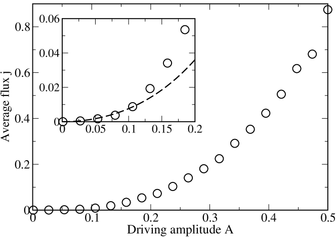
Figure 1: Average energy flux vs. driving amplitude for in-band forcing, $\omega=1.8$, $\gamma=5$. Data have been averaged over $10^{5}$ periods of the driving. The inset is an enlargment of the small-amplitude region and the dashed line is the single nonlinear phonon approximation (7).

IV Out-band driving: supratransmission

Let us now turn to the more interesting case in which the driving frequency lies outside the phonon band, $\omega>\omega_{0}(\pi,0)=2$. In a first series of numerical experiments we have initialized the chain at rest and switched on the driving at time $t=0$. To avoid the formation of sudden shocks shocks , we have chosen to increase smoothly the amplitude from 0 to the constant value $A$ at a constant rate, i.e.

$$u_{0}=A\cos(\omega t)\left[1-e^{-t/\tau_{1}}\right]~{},$$ (8)

where typically we set $\tau_{1}=10$.

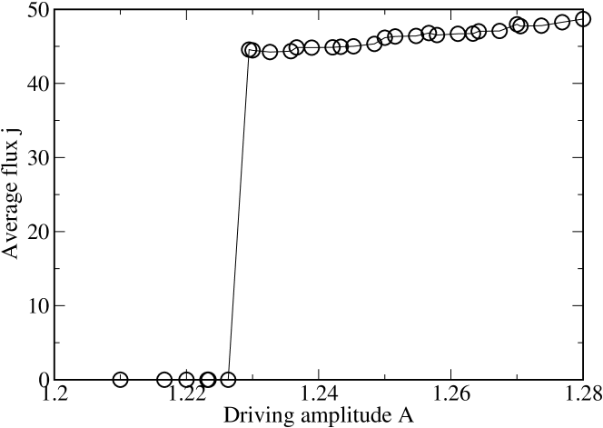
Figure 2: Average energy flux vs. driving amplitude for out–band forcing, $\omega=3.5$, $\gamma=5$. Data have been averaged over $2\,10^{5}$ periods of the driving for a chain of $N=512$ particles.

At variance with the case of in–band forcing, we observe a sharp increase of the flux at a given threshold amplitude of the driving, see Fig. 2. This phenomenon has been denoted as nonlinear supratransmission leon to emphasize the role played by nonlinear localized excitations in triggering the energy flux.

This situation should be compared with the one of in–band driving, shown in Fig. 1, where no threshold for conduction exists and the flux increases continuously from zero (more or less quadratically in the amplitude). Indeed, the main conclusion that can be drawn from the previous section is that there cannot be any amplitude threshold for energy transmission in the case of in-band forcing. Moreover, although at the upper band edge the flux vanishes, since it is proportional to the group velocity (see formula (7)), it is straightforward to prove that it goes to zero with the square root of the distance to the band edge frequency. Hence, the sudden jump we observe in the out-band case cannot be explained by any sort of quasi-linear approximation.

In the following we investigate the physical origin of nonlinear supratransmission, distinguishing the cases of small and large amplitudes.

Figure 3: Snapshot of the local energy below the supratransmission threshold $A=0.15<A_{th}$ for $\omega=2.1$ $\gamma=10$. The initial condition is an envelope soliton (11) with $x_{0}=-1.8$ (above) and $x_{0}=+1.8$ (below).

IV.1 Small amplitudes

When the driving frequency is only slightly above the band ($0<\omega-2\ll 1$), one can resort to the continuum envelope approximation. Since we expect the zone–boundary mode $k=\pi$ to play a major role, we let

$$u_{n}\;=\;(-1)^{n}\frac{1}{2}\left[\psi_{n}\,e^{i\omega t}+\psi_{n}^{*}\,e^{-i\omega t}\right]~{}.$$ (9)

In the rotating wave approximation rwa and for slowly varying $\psi_{n}$ one obtains from the FPU lattice equations the nonlinear Schrödinger equation ($\psi_{n}\longrightarrow\psi(x,t)$) scott

$$2i\omega\dot{\psi}\;=\;(\omega^{2}-4)\psi-\psi_{xx}-12\psi|\psi|^{2}~{},$$ (10)

with the boundary condition $\psi(0,t)=A$.

The well-known static single–soliton solution of Eq. (10) corresponds to the family of envelope solitons (low-amplitude discrete breathers)

$$u_{n}\;=\;a(-1)^{n}\cos(\omega t)\,{{\rm sech}\left[\sqrt{6}(n-x_{0})a\right]},$$ (11)

with amplitude $a=\sqrt{(\omega^{2}-4)/6}$. The maximum of the soliton shape is fixed by the boundary condition to be

$$x_{0}\;=\;\pm{{\rm acosh}(a/A)\over a\sqrt{6}}~{}.$$ (12)

In this approximation we have two possible solutions: one with the maximum outside the chain, which is purely decaying inside the chain (minus sign in (12)), and another with the maximum located within the chain (plus sign in (12)). Overcoming the supratrasmission threshold corresponds to the disappearence of both solutions. Indeed, when the driving amplitude reaches the critical value $A_{th}$, given by

$$\omega^{2}=4+6A_{th}^{2}~{},$$ (13)

solution (11) ceases to exists.

Figure 4: Snapshot of the local energy at the transmission threshold $A=0.253\approx A_{th}$ for $\omega=2.1$ $\gamma=10$. The initial condition is the envelope soliton (11) with $x_{0}\approx 0$.

We have investigated this issue by simulating the lattice dynamics with the initial conditions given by Eqs. (11) and (12). The evolution of the local energy

$$e_{n}\;=\;{\dot{u}^{2}_{n}\over 2}+\frac{1}{2}\left[V(u_{n+1}-u_{n})+V(u_{n}-u_{n-1})\right]$$ (14)

with $V(x)=x^{2}/2+x^{4}/4$, is shown in Fig. 3. The solution with the maximum outside the chain (upper figure) stabilizes after the emission of a small amount of radiation (generated by the fact that we have used an approximate solution). On the contrary, the other solution (lower figure) slowly moves towards the right and, eventually, leaves a localized boundary soliton behind. The release of energy to the chain is non stationary and does not lead to a conducting state.

The scenario drastically changes at the supratransmission amplitude $A_{th}$. The chain starts to conduct: a train of travelling envelope solitons is emitted from the left boundary (see Fig. 4). Here we should emphasize that the envelop soliton solution (11), which is characterized by the $k=\pi$ carrier wave–number, has a zero group velocity. Thus, transmission cannot be realized by such envelope solitons. Instead, transmission starts when the driving frequency resonates with the frequency of the envelope soliton with carrier wave–number $k=\pi(N-2)/N$, next to the $\pi$-mode. However, as far as we consider a large number of oscillators ($N=500$), we can still use expression (13) for the $\pi$-mode frequency.

IV.2 Large amplitudes

The above soliton solution is valid in the continuum envelope limit, and is therefore less and less accurate as its amplitude increases. Indeed, if the weakly nonlinear condition is violated, the width of the envelope soliton becomes comparable with lattice spacing and, thus, one cannot use the continuum envelope approach. Fortunately, besides the slowly varying envelope soliton solution (11), an analytic approximate expression exists for large amplitude static discrete breather solutions, which is obtained from an exact extended plane wave solution with “magic” wave–number $2\pi/3$ kosprl

$$u_{n}=a(-1)^{n}\cos\left[\omega_{B}(a)t\right]\cos\left(\frac{\pi}{3}n\pm x_{0}\right)~{},$$ (15)

if $\left|(\pi n/3)\pm x_{0}\right|<\pi/2$ and $u_{n}=0$ otherwise.

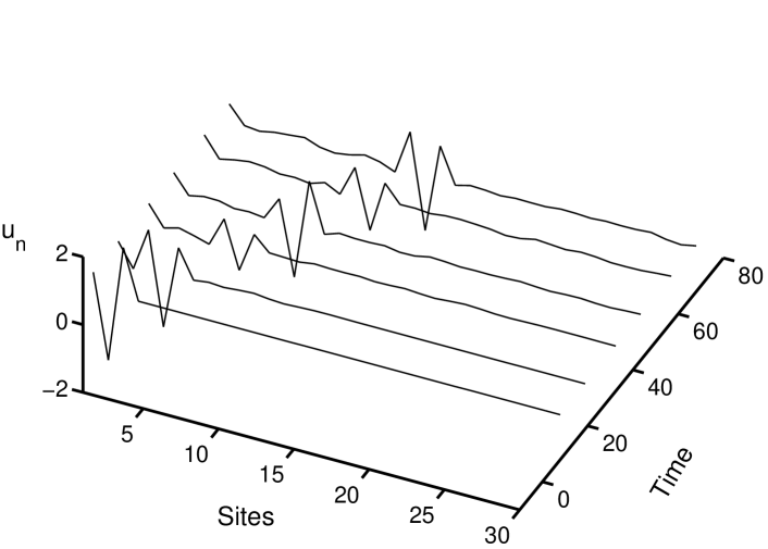
Figure 5: Snapshot of particle displacements $u_{n}$ below the supratransmission threshold for a driving frequency $\omega=5.12$ and a driving amplitude $A=0.5<A_{th}=2.05$. One can observe, similarly to the lower Fig. 3, that a moving discrete breather appears at the left boundary and propagates inside the bulk, leaving behind the static solution.

Here $x_{0}$ is defined as follows

$$x_{0}=\mbox{acos}(A/a)~{},$$ (16)

where $A$ is the driving amplitude. The breather frequency $\omega_{B}(a)$ depends on amplitude $a$ as follows

$$\omega_{B}(a)\simeq 1.03\frac{\sqrt{3\pi^{2}(4+9a^{2})}}{4K(s)},$$ (17)

where $K(s)$ is the complete elliptic integral of the first kind with argument $s=3a/\sqrt{2(9a^{2}+4)}$ and the factor $1.03$ takes into account a rescaling of the frequency of the “tailed” breather note (see also kos ). As previously for the case of the envelope soliton solution, we perform a numerical experiment where we put initially on the lattice the breather solution of formula (15). Choosing the plus sign in this expression, we do not observe any significant transmission of energy inside the chain. Instead, the minus sign causes the appearance of a moving breather, which travels inside the chain leaving behind the static breather solution with plus sign. Fig. 5 presents this numerical experiment.

The static breather solution (15) ceases to exist if the driving amplitude exceeds the threshold $A_{th}$ given by the resonance condition

$$\omega=\omega_{B}(A_{th}).$$ (18)

Above this threshold the supratransmission process begins via the emission of a train of moving breathers from the boundary, exactly as it happens in the case of small amplitudes. It should be mentioned again that the transmission regime is established due to moving discrete breathers. It has been remarked kosprl that discrete breathers are characterized by quantized velocities, while their frequency is given by the same formula (17). This explains why one can use resonance condition (18) for the static discrete breather solution (15) to define the supratransmission threshold in the large amplitude limit.

IV.3 Supratransmission threshold: numerical test

To check these predictions, we have performed a numerical determination of $A_{th}$ for several values of $\omega$, starting the chain at rest. This is accomplished by gradually increasing $A$ and looking for the minimal value $A_{th}$ for which a sizeable energy propagates into the bulk of the chain. At early time, the scenario is qualitatively similar to the one shown in Fig.4. Later on, the interaction of nonlinear and quasi-linear modes and their “scattering” with the dissipating right boundary establishes a steady energy flux into the chain. A conducting steady state, which is present also below $A_{th}$, will be discussed in Section V in connection with a lower-transmission threshold $A_{th}^{-}$.

As seen in Fig. 6, formulae (18) [with definition (17)] and (13) (see the inset) are in excellent agreement with simulations for large $A>2$ and small $A\lesssim 1$ amplitudes, respectively. The accuracy of the analytical estimate in formulae (18) and (13) is of the order of few percents, at worst, in the intermediate amplitude range. We don’t discuss here the lower curves in Fig. 6, which are related to the lower-transmission threshold.

For comparison, we have checked that the supratransmission threshold is definitely not associated with the quasi-harmonic waves with nonlinear dispersion relation (5). If this were the case, the transmission should start when the oscillation amplitude reaches the value for which the resonance condition $\omega=\omega_{0}(k,A)$ holds. As $\omega_{0}(k,A)$ is maximal for $k=\pi$, we can get the expression for the threshold value from the relation $\omega=\omega_{0}(\pi,A_{th})$, i.e.

$$\omega^{2}=4+12A_{th}^{2}.$$ (19)

The amplitude values one obtains from Eq. (19) are far away from the numerical values and we don’t even show them in Fig. 6. This is a further confirmation that supratransmission in the FPU model originates from direct discrete breather generation as it happens in the cases of discrete sine-Gordon and nonlinear Klein-Gordon lattices leon .

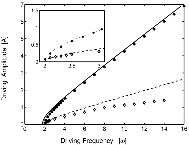
Figure 6: Comparison between analytic estimates and numerical values of threshold amplitudes vs. the driving frequency. Main plot: the full dots are the numerical values of $A_{th}$ and the solid line is a plot of formulae (17-18), which are valid for large amplitudes. The inset shows an enlargement of the small $A_{th}$ region, in order to illustrate the accuracy of the small-amplitude approximation (13) (dotted line). The diamonds are simulation data for the lower-transmission threshold $A_{th}^{-}$ and the dashed line is formula (22). Notice how the latter is accurate only for small enough amplitudes (see again the inset).

V Stationary states

As announced in the Introduction, we have also investigated the long-time behavior of the chain. As shown in the upper Fig. 7 the time averaged local energy (see formula (14)) reaches asymptotically a given profile: local energy monotonously decreases along the chain as in the case of simulations of stationary heat transport with two thermal baths rep . The time–average of the flux (3) in the stationary state is almost constant along the chain, apart from statistical fluctuations and some persistent flux oscillations at the left boundary.

However, as we mentioned above, the value of the stationary flux depends on the initial state of the chain. To illustrate this effect, let us excite the chain imposing a different boundary condition

$$u_{0}=\cos(\omega t)\left[B(1-e^{-t/\tau_{1}})+(A-B)(1-e^{-t/\tau_{2}})\right]$$ (20)

where $\tau_{2}\gg\tau_{1}$ (in the experiment $\tau_{2}=10\tau_{1}=100$), $A<A_{th}$ and $B>A_{th}$. Obviously, both the boundary condition (8) and (20) lead to the same driving amplitude $A$ for $t\gg\tau_{2}$. However, at variance with (8), when imposing (20), the istantaneous forcing amplitude overcomes the critical amplitude $A_{th}$ for a time of the order of $\tau_{2}$, which is enough to establish a stationary flux regime. This drastically reduces the transmission threshold to a value $A_{th}^{-}<A_{th}$, which we denote as lower-transmission threshold. This is the first observation of this phenomenon, of which we will give a theoretical interpretation in the following. The numerical determination of $A_{th}^{-}$ versus the driving frequency $\omega$ is reported with diamonds in Fig. 6.

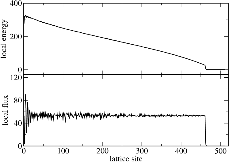
Figure 7: Time–averaged local energy (above) and energy flux (below) versus lattice position in the case of out-band driving, $\omega=3.5$, $A=1.27$. The 50 rightmost particle out of $N=512$ have been damped with $\gamma=5$. The averages are taken over $2\,10^{5}$ driving periods .

In the amplitude interval $[A_{th}^{-},A_{th}]$, two steady states coexist, a conducting state and an insulating one. Each of the two steady states can be attained with different initial conditions of the chain and different driving pathways. For instance, the conducting state is reached when imposing driving (20), the insulating one when using (8). It is a typical bistable situation, where two (possibly chaotic) attractors coexist in a given control parameter range.

This behaviour is illustrated in Fig.8 using a different simulation method. The average flux is computed after changing $A$ stepwise. A back and forth sweep around the amplitude interval $[A_{th}^{-},A_{th}]$ reveals the presence of the two states.

A justification of the presence of the lower-trasmission threshold can be given in terms of quasi-linear theory. This theory leads to dispersion relation (5) only if one restricts to a single right-propagating mode. However, due to reflection with the boundary and to mode interaction, both the right-propagating mode and the left-propagating one can contribute to the dispersion relation. In the Appendix, we derive this more general dispersion relation. After introducing the complex mode amplitude $a_{k}$ for the $k$-th mode, the dispersion relation takes the following form

$$\omega(k)^{2}=2(1-\cos k)+3(1-\cos k)^{2}\left[|a_{k}|^{2}+2|a_{-k}|^{2}\right]~{}.$$ (21)

In order to fulfill the resonance condition with both the right-propagating ($a_{k}$) and the left-propagating ($a_{-k}$) mode, their amplitudes must be equal $|a_{k}|=|a_{-k}|$. Since $\omega(k)$ is maximal for $k=\pi$, the condition for the threshold amplitude is

$$\omega^{2}\;=\;4+36\left(A_{th}^{-}\right)^{2}.$$ (22)

This analytical estimate (dashed line in Fig. 6) fits well the numerical data only for driving frequencies close to the band edge (see the inset). This can be justified by taking into account that dispersion relation (21) is valid only in the weakly nonlinear regime, i.e. mode amplitudes $|a_{k}|$ and $|a_{-k}|$ much smaller than $1$. This condition certainly applies to the case in which the driving frequency is close to the band edge, since, then, the threshold amplitude $A_{th}^{-}$ is small. When the driving frequency is far from the band edge, one has to take into account higher-order corrections. The inclusion of the first “satellite” mode ($3k$) produces a lower threshold amplitude, but the agreement with numerical data extends only to slightly larger amplitudes. To obtain a definitely better agreement, one should treat all satellite modes $5k$, $7k$, etc.. We briefly discuss this aspect in the Appendix.

From the above considerations, it follows that the bistable nature of the energy flux can be explained making reference to the different excitations of the system. Indeed, with the system initially at rest, when following the driving method (8), extended quasi-harmonic waves cannot be excited. Then, energy flow appears only when the driving amplitude reaches the value necessary for localized mode excitation. On the other hand, with driving (20), the energy flow is initiated by the overcoming of the supratransmission threshold and then sustained also by extended quasi-harmonic waves.

It is also possible to give a heuristic argument to explain why the transition from non zero to zero flux is “continuous” at the lower-transmission threshold $A_{th}^{-}$, while there is flux jump at the supratransmission threshold $A_{th}$. When the quasi-harmonic waves are already excited, reducing the driving amplitude diminishes also the number of resonating modes continuously. Hence, the flux goes continuously to zero proportionally to this number, producing a sort of second-order phase transition, when the flux is considered as an order parameter. On the contrary, when increasing the driving amplitude with the lattice at rest across the supratransmission threshold $A_{th}$, localized modes are excited, which successively excite also extended waves. Hence, a non zero flux is created suddenly from the zero flux state, generating a sort of first-order phase transition.

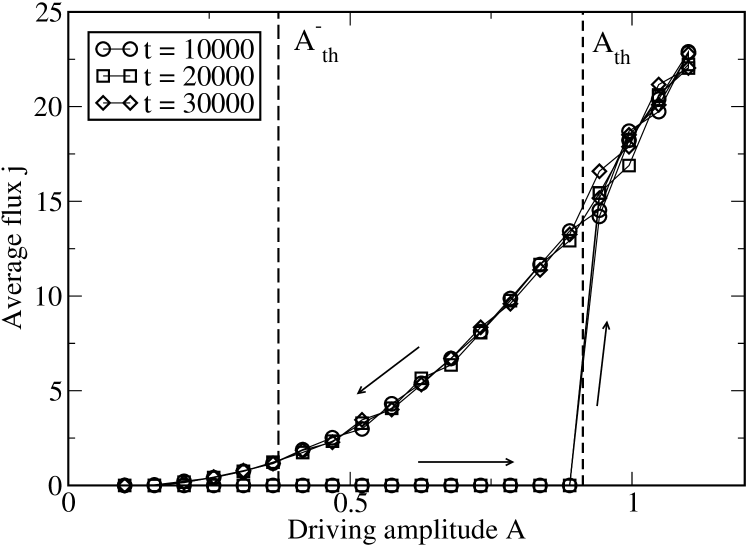
Figure 8: Energy flux versus driving amplitude for $\omega=3$, $N=512$, $\gamma=5$. The coexistence of the conducting and insulating regimes is revealed by sweeping the forcing amplitude in the range $[A_{th}^{-},A_{th}]$. The sweeping direction is indicated by the arrows. The analytical values of the two thresholds are indicated by the vertical dashed lines. While the prediction for the supratransmission threshold $A_{th}$ is quite good, the one for the lower-transmission threshold $A_{th}^{-}$ overestimates the numerical value (the prediction becomes better for smaller driving frequencies, as shown in Fig. 6). In order to show that the steady state is already reached for these integration times, results for increasing averaging times are displayed with different symbols.

VI Conclusions and perspectives

We have discussed the supratransmission phenomenon for the Fermi-Pasta-Ulam one-dimensional lattice. A theory, based on a resonance condition of the driving frequency with the typical frequency of localized excitations (solitons, breathers), gives a good agreement of the supratransmission threshold with numerical data. Below this threshold two steady states coexist, a conducting and an insulating one. For even lower driving amplitudes a further transition occurs to a region where only the insulating state persists: we have called this new phenomenon lower-transmission threshold. Imposing a resonance condition for nonlinear quasi-harmonic waves, we are able to derive an analytic expression for the lower-transmission threshold amplitude.

At the supratransmission threshold a jump in the energy flux appears. This is reminiscent of a first-order phase transition. At variance, at the lower-transition threshold the flux goes to zero continuously. This analogy with non-equilibrium phase transitions mukamel should be further explored.

Fluctuations in steady states could be analysed to verify the possible role played by the Gallavotti-Cohen out-of equilibrium fluctuation theorem gallavotti .

The supratransmission phenomenon is quite generic and has already been observed experimentally in a chain of coupled pendula leon2 . Also the bistability of conducting/insulating states is generic and could be observed experimentally in similar conditions. For instance, one could apply this theory to micromechanical experiments of the type performed by Sievers and coworkers sievers .

Appendix A Nonlinear phonon dispersion

In order to derive the nonlinear dispersion relation for extended quasi-harmonic waves, let us seek for the solutions of the equations of motion (1) of the form

$$u_{n}=\frac{1}{2}\sum\limits_{p}\left[a_{p}e^{i(\omega(p)t+pn)}+a_{-p}^{+}e^{-i(\omega(p)t-pn)}\right]~{},$$ (23)

where $\omega(p)$ is the frequency of the $p$-th mode and $a_{p}$ its complex amplitude. Substituting this Fourier expansion into the equations of motion, one gets the following infinite set of algebraic equations for mode amplitudes raleru

$$\left[\omega(p)^{2}-2(1-\cos p)\right]a_{p}=6\sum\limits_{q_{1},q_{2}}G_{q_{1},q_{2}}^{p}a_{q_{1}}a_{q_{2}}a_{q_{1}+q_{2}-p}^{+},$$ (24)

where

$$G_{q_{1},q_{2}}^{p}=\frac{1}{4}[1+\cos(q_{1}+q_{2})+\cos(p-q_{2})+\cos(p-q_{1})$$

$$-\cos p-\cos q_{1}-\cos q_{2}-\cos(p-q_{1}-q_{2})].$$

If only a single mode $p=k$ is excited, one gets the following dispersion relation

$$\omega(k)^{2}=2(1-\cos k)+3(1-\cos k)^{2}|a_{k}|^{2},$$ (25)

which has been introduced in Eq. (5).

On the other hand, when both mode $k$ and mode $-k$ are excited, one obtains

$$\omega(k)^{2}=2(1-\cos k)+3(1-\cos k)^{2}\left[|a_{k}|^{2}+2|a_{-k}|^{2}\right]~{},$$ (26)

which is presented as Eq. (21) in the text.

As also mentioned in the text, one must sometimes consider the excitation of “satellite” modes $3k$, $5k$, etc.. The inclusion of the $3k$ mode produces the addition of the following term

$$3\left[3\cos^{2}k-1-2\cos^{3}k\right]\left(|a_{-k}|^{4}+2|a_{-k}|^{2}|a_{k}|^{2}\right),$$ (27)

to the r.h.s of Eq. (26). This gives the following resonance condition at $k=\pi$

$$\omega^{2}=4+36(A_{th}^{-})^{2}\left(1+\frac{12(A_{th}^{-})^{2}}{\omega^{2}-4}\right)~{},$$

where $\omega$ and $A_{th}^{-}$ are the driving frequency and lower-threshold amplitude, respectively. Since the coefficient of the $(A_{th}^{-})^{4}$ term in this relation is always positive, the threshold amplitude one obtains is smaller that the one derived from Eq. (22) in the text.

References

- (1) F. Geniet, J. Leon, Phys. Rev. Lett., 89, 134102, (2002).
- (2) F. Geniet, J. Leon, J. Phys.: Condens. Matter, 15, 2933 (2003).
- (3) J. Leon and A. Spire, arXiv:nlin.PS/0310006.
- (4) J. Leon, Phys. Lett. A, 319, 130 (2003).
- (5) R. Khomeriki, Phys. Rev. Lett., 92, 063905 (2004).
- (6) E. Fermi, J. Pasta, S. Ulam, M. Tsingou, in The Many-Body Problems, edited by D.C. Mattis (World Scientific, Singapore, 1993 reprinted).
- (7) S. Flach and C.R. Willis, Phys. Rep., 295, 181 (1998).
- (8) Yu. A. Kosevich, Phys. Rev. Lett. 71, 2058 (1993) and Phys. Rev. B, 47, 3138, (1993).
- (9) S. Lepri, R. Livi, A. Politi, Phys. Rep., 377, 1, (2003).
- (10) S. Takeno, K. Kisoda, A.J. Sievers, Prog. Theor. Phys. Suppl., 94, 242, (1988).
- (11) Yu. A. Kosevich, R. Khomeriki, S. Ruffo, Europhys. Lett., 66, 21 (2004).
- (12) A. Scott, Nonlinear science, Oxford University Press (1999), Chapter 3.3..
- (13) R. Khomeriki, Phys. Rev. E, 65, 026605, (2002).
- (14) Notice that a simpler approximate expression for the breather frequency has been proposed in kosprl in the form . We have checked that this expression is also in good agreement with numerical data, but we prefer to use the more accurate form in formula (17).
- (15) Yu. A. Kosevich, G. Corso, Physica D, 170, 1, (2002).
- (16) R. Khomeriki, S. Lepri, S. Ruffo, Phys. Rev. E., 64, 056606, (2001).
- (17) D. Mukamel, in Soft and fragile matter: non-equilibrium dynamics, metastability and flow, Eds. M.E. Cates and M.R. Evans (Bristol, IOP Publishing)(2000).
- (18) G. Gallavotti and E.G.D. Cohen, J. Stat. Phys, 80, 931 (1995).
- (19) M. Sato et al., Phys. Rev. Lett., 90, 044102 (2003).