THERMAL EFFECTS IN PHOTOEMISSION AND ELECTRON-PHONON COUPLINGS OF FULLERENE

Abstract

We show that thermal effects play a relevant role in the determination of the electron-phonon couplings based on the intensity of the phonon-shakeup peaks in photoemission spectra. In particular, we re-consider the determination of the electron-phonon couplings of fullerene based on a fit of the photoemission spectrum of C${}_{60}^{-}$ in gas phase [1]. We show that taking thermal effects into account reduces the obtained couplings by approximately 10%.

1 INTRODUCTION

Many of the interesting phenomena observed in electron-donor doped fullerides are related to electron-phonon coupling of the partly filled band derived from the lowest unoccupied molecular orbital (LUMO) of C₆₀. These couplings, in turn, are mainly of molecular origin, involving the optical phonons derived from the molecular modes of $A_{g}$ and $H_{g}$ symmetry. Several different determinations of the electron-phonon couplings of the LUMO are available on the market, both from calculations [2, 3, 4, 5], and derived from experimental data [1]. All calculations based on density-functional theory (DFT) invariably turn out much smaller couplings than those obtained through fitting the experimental photoemission spectrum (PES) of gas-phase C${}_{60}^{-}$ (see for example Table 1). This spectrum is affected by the electron-phonon shakeup associated to relaxation after the sudden ejection of the extra electron from the LUMO. That fit was realized on the basis of a zero-temperature model for the electron-phonon coupled system. The authors of Ref. 1 estimate the vibrational temperature of the sample ions of the order of 200 K. We claim that even such a low temperature could affect significantly the spectrum, in a way not unlike an increase of the couplings. We conclude that a determination of the couplings via a model including realistic thermal effects must turn out smaller couplings than a zero-temperature model.

Mode(j)	Exp. freq. (cm-1)	DFT Energy (meV)	$g_{\Lambda_{j}}$ PES[1]	$g_{\Lambda_{j}}$ DFT[5]
$A_{g}^{(1)}$	496		0.0	0.157
$A_{g}^{(2)}$	1470		0.851	0.340
$H_{g}^{(1)}$	271	32	0.824	0.412
$H_{g}^{(2)}$	437	53	0.941	0.489
$H_{g}^{(3)}$	710	89	0.421	0.350
$H_{g}^{(4)}$	774	97	0.474	0.224
$H_{g}^{(5)}$	1099	139	0.325	0.193
$H_{g}^{(6)}$	1250	158	0.197	0.138
$H_{g}^{(7)}$	1428	180	0.339	0.315
$H_{g}^{(8)}$	1575	197	0.376	0.289

Table 1: Experimental frequencies of the vibrational modes of fullerene linearly coupled to the $t_{1u}$ LUMO. Computed energies and dimensionless coupling constants.

2 THE MODEL

The standard formulation of the linear electron-phonon model [6, 7, 1] describing the JT coupling of the orbitally degenerate $t_{1u}$ molecular triplet with the vibrations of symmetry $\Lambda=A_{g},\,H_{g}$ is the following:

$$\hat{H} = \hat{H}_{0}+\hat{H}_{\rm vib}+\hat{H}_{\rm e-v}\,,$$ (2.1)

$$\hat{H}_{0} = \epsilon\,\sum_{m\sigma}\hat{c}_{m\sigma}^{\dagger}\hat{c}_{m\sigma}\,,$$ (2.2)

$$\hat{H}_{\rm vib} = \frac{1}{2}\sum_{j\mu}\hbar\omega_{\Lambda j}\left(\hat{P}_{j\mu}^{2}+\hat{Q}_{j\mu}^{2}\right)\,,$$ (2.3)

$$\hat{H}_{\rm e-v} = \,k^{\Lambda}\sum_{{\sigma\,\mu mm^{\prime}}}C^{\Lambda\mu}_{m\;-m^{\prime}}\,\sum_{j}g_{\Lambda j}\hbar\omega_{\Lambda j}\hat{Q}_{j\mu}\,\hat{c}^{\dagger}_{m\sigma}\hat{c}_{m^{\prime}\sigma}\,.$$ (2.4)

Here, $\hat{Q}_{j\mu}=\left(\hat{b}_{j\mu}^{\dagger}+\hat{b}_{j\mu}\right)/\sqrt{2}$ is the dimensionless normal-mode vibrational coordinate (in units of the natural length scale of the harmonic oscillator), and $\hat{P}_{j\mu}$ the corresponding conjugate momentum for mode $j$ of symmetry $\Lambda$ (either $A_{g}$: 2 modes, or $H_{g}$: 8 modes). $\hat{c}^{\dagger}_{m\sigma}$ is a fermion operator creating a spin-$\sigma$ electron in orbital $m=0,\pm 1$ of the LUMO. $m$, $m^{\prime}$ and $\mu$ label components within the degenerate multiplets, for example according to the $C_{5}$ character in the ${\cal I}\supset D_{5}\supset C_{5}$ group chain [8, 9]. In particular, $\mu=0,\pm 1,\pm 2$ for $H_{g}$ modes and $\mu=0$ only for $A_{g}$ modes. $C^{\Lambda\mu}_{mm^{\prime}}$ are Clebsch-Gordan coefficients [9] of the icosahedral group ${\cal I}$ that couple two $t_{1u}$ tensor operators and a $\Lambda$ tensor operator to a global scalar $A$ operator (in practice these coefficients equal spherical Clebsch-Gordan coefficients for coupling two $l=1$ angular momenta to $L=0$ for $\Lambda=A_{g}$ and $L=2$ for $\Lambda=H_{g}$). Numerical factors $k^{A}=\sqrt{3}$, $k^{H}=\sqrt{3/2}$ (which could otherwise be re-absorbed into the definition of $g_{\Lambda j}$) are included to make contact with previous notation [7, 5]. $g_{\Lambda j}$ are precisely the electron-phonon coupling parameters whose determination is addressed in this work.

The $H_{g}$-mode coupling in the model [2.1] is of the Jahn-Teller (JT) type: exact solution are known only for very large or very small couplings. The couplings of fullerene appear to be in an intermediate regime, for which only numerical solutions are available. Indeed, the authors of Ref. 1, applied Lanczos diagonalization to the Hamiltonian [2.1] on a truncated harmonic basis, to obtain its ground state. The analysis of this ground state in terms of the harmonic ladder of oscillators of the non-JT neutral C₆₀ provided the intensities to reconstruct the spectrum. At any finite temperature one should in principle repeat the analysis not only for the JT ground state, but also for a number of low-lying excitations and sum the resulting spectra, each multiplied by the corresponding Boltzmann weight. An attempt to follow this route at any finite temperature such that $k_{B}T$ is comparable to even the lowest quanta of vibration ($\approx 30$ meV) is beyond the possibilities of nowadays computers, due to the large number of oscillators, and the associated rapidly increasing density of coupled states: a reliable evaluation of the spectrum would require the accurate determination of the wavefunction of several hundred thousand of the lowest states in a Hilbert space of several million.

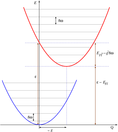
Figure 1: The schematic “Frank-Condon” structure of the PES experiment, as seen from the point of view of any given normal-mode coordinate $Q$. Along each normal-mode direction, the displacement of the minimum of the ionized configuration with respect to that of the neutral configuration is proportional to the coupling of that mode.

We propose here a more efficient method, based on a related much simpler model, for which an analytical solution allows to carry out the calculation even to fairly high temperature, with mild computational requirements. The basic observation here is that in the experiment under examination the final states (neutral C₆₀) involve simple harmonic ladders of phonons. These are excited by an amount which is related to the displacement of the adiabatic minimum of the initial C${}_{60}^{-}$ with respect to that of the final C₆₀, as illustrated in Fig. 1. The intricate details of the initial JT state should play only a minor role in this spectrum, the main thing that needs to be made right being the displacement between the two minima. We replace therefore each of the $H_{g}$ modes (with the complication of the full JT Hamiltonian [2.1]) with a set of five effective $A_{g}$ modes, with the same frequency as the original fivefold-degenerate mode, and a suitable coupling $g_{A}^{\rm eff}$. It is important to introduce 5 degenerate oscillators per mode, to reproduce correctly the increasing density of oscillator states with energy, which is crucial to describe thermal effects. The advantage of $A_{g}$ nondegenerate oscillators is that their wavefunction expansion on a displaced basis is known analytically. Note that this approximation could not possibly work in a context (such as that of the PES from neutral C₆₀ [10, 11]) where the final states are affected by JT.

Briefly, starting from an initial state $|i\rangle=|v\rangle$ with $v$ quanta in the initial state, the required probability amplitude to end up into a final state $|f\rangle=T^{-a}|w\rangle$ ($\hat{T}^{-a}$ is a space translation operator and the distance $a=\frac{1}{2}\,g_{A}$) with $w$ quanta is

$$\langle f|\hat{c}_{m\sigma}^{\dagger}|i\rangle=\langle\varphi_{w}|T^{a}|\varphi_{v}\rangle=\sqrt{\frac{2^{v}\,v!}{2^{w}\,w!}}\;e^{-\frac{1}{4}a^{2}}\,a^{w-v}\,L_{v}^{w-v}\!\left(\frac{a^{2}}{2}\right)$$ (2.5)

where $L_{r}^{\lambda}(z)$ are the Laguerre polynomials of degree $r$: $L_{r}^{\lambda}(z)\!=\!\frac{z^{-\lambda}e^{z}}{r!}\frac{\mathrm{d}^{r}}{\mathrm{d}z^{r}}\Big{(}z^{r+\lambda}e^{-z}\Big{)}$. The spectral function is then computed according to Fermi’s golden rule in the sudden approximation:

$$I_{i}(h\nu)=\frac{2\pi}{\hbar}\sum_{f}|\langle f|V_{I}|i\rangle|^{2}\delta(h\nu-(E_{f}-E_{i})),$$ (2.6)

where $E_{i}$ and $E_{f}$ have trivial harmonic expressions. Assuming a Boltzmann population of the initial states

$$P(i)=\frac{\exp\left[-\frac{E_{i}}{k_{\rm B}T}\right]}{\sum_{l}\exp\left[-\frac{E_{l}}{k_{\rm B}T}\right]}\,,$$ (2.7)

the final spectrum is obtained through the following thermal average:

$$I(h\nu)=\sum_{i}P(i)\,I_{i}(h\nu)\,.$$ (2.8)

In the problem of C₆₀ at hand, the total number of oscillators is $5\times 8+2=42$. To combine the spectral contributions of individual oscillators, the collective matrix element in [2.6] is the product of the matrix elements of the individual oscillators, while the position $(E_{f}-E_{i})$ of the peak is of course the sum of the energy change of the individual oscillators:

$$\langle f|V_{I}|i\rangle\!\!\! = \!\!\!\langle w_{1},w_{2},...|V_{I}|v_{1},v_{2}\rangle=\langle w_{1}|T^{a_{1}}|v_{1}\rangle\langle w_{2}|T^{a_{2}}|v_{2}\rangle...$$ (2.9)

$$E_{f}-E_{i}\!\!\! = \!\!\!(E_{w_{1}}+E_{w_{2}}+...)-(E_{v_{1}}+E_{v_{2}}+...)=$$

$$= \!\!\!(E_{w_{1}}-E_{v_{1}})+(E_{w_{2}}-E_{v_{2}})+...$$

The delta-function peaks are finally broadened into Gaussians of 20 meV HWHM to account for the final resolution of the spectrometer. For more details on this simple model, the reader is referred to Ref. 12.

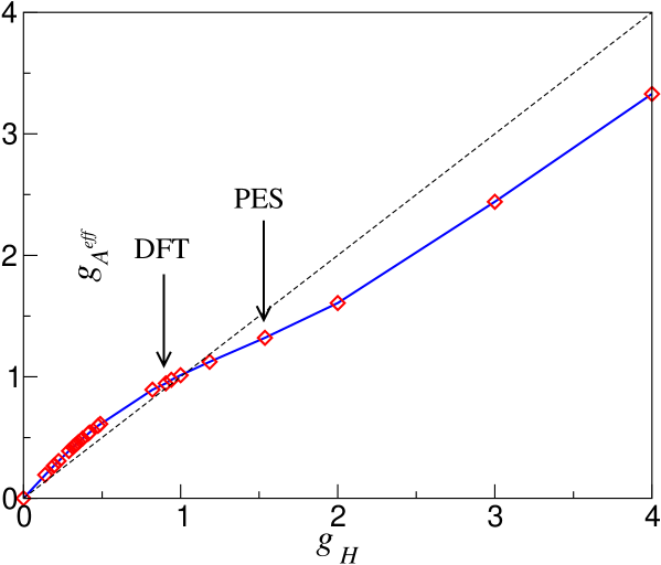
Figure 2: The best fit value of $g_{A}^{\rm eff}$ as a function of $g_{H}$, according to a $T=0$ calculation. Arrows point to the values of the total $\overline{g}_{H}$ according to the DFT [5] and PES [1] estimates.

To determine the value of the effective couplings $g_{A_{j}}^{\rm eff}$, we fit the $T=0$ spectrum of a single $H_{g}$ mode (computed by exact Lanczos diagonalization of [2.1]) with that of 5 degenerate $A_{g}$ oscillators of the same frequency. By repeating this fit for a range of couplings, we obtain the curve of Fig. 2. We have then verified that the temperature dependence of the spectrum based on the zero-temperature fit is in very good accord to that obtained by exact diagonalization (which, for this single-mode case, can be carried out up to moderately high temperature).

Figure 3: $T=0$ comparison between the exact JT Lanczos spectrum (solid line) and that obtained by the simplified effective-$A$ modes model (dashed line). Comparison done for PES couplings [1], Gaussian broadening of 10 meV HWHM, including only $H_{g}$ modes.

For treating many modes, it is necessary to take into account the “collective” nature of the JT interaction. Therefore, instead of converting each individual $g_{Hj}$ through the relation of Fig. 2, we consider the “total coupling” [13, 14] $\overline{g}_{H}=\left(\sum_{j}g_{Hj}^{2}\right)^{1/2}$, and convert $\overline{g}_{H}$ into a $\overline{g}_{A}^{\rm eff}$, through Fig. 2. We then multiply each individual $g_{Hj}$ by the same ratio $\overline{g}_{A}^{\rm eff}/\overline{g}_{H}$, to obtain the effective $g_{Aj}^{\rm eff}$ couplings for each mode. For the DFT coupling reported in Table 1, the ratio $\overline{g}_{A}^{\rm eff}/\overline{g}_{H}=1.045$, while for the PES couplings $\overline{g}_{A}^{\rm eff}/\overline{g}_{H}=0.859$. On the basis of these couplings, we compute the $T=0$ spectrum, and in both cases we obtain a good accord with the exact Lanczos calculation. Figure 3 illustrates this comparison for the PES couplings.

3 RESULTS AND DISCUSSION

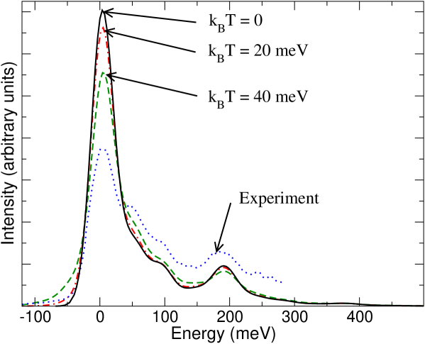
Figure 4: All-modes PES computed based on the effective-$A$ modes model at $k_{B}T$=$20$ and $40$ meV, for the DFT couplings of Ref. 5. The poor accord with experiment indicates that, even accounting for thermal effects, the DFT couplings are indeed too small to account for the observed transfer of spectral weight to the phonon satellites.

We apply now the effective-$A$ modes model to the computation of the PES at finite temperature. Figure 4 reports the thermal spectrum for realistic values $k_{B}T=20$, 40 meV, computed on the basis of the DFT parameters [5], rescaled as discussed above. Clearly, even though thermal effects go in the direction of increasing the transfer of weight to the phonon excitation and reducing the distance to the experimental spectrum, the agreement remains poor, thus confirming that the DFT parameters are indeed too small. There is not a satisfactory explanation yet for this failure of DFT, which is particularly surprising in light of the accurate values for the couplings of the HOMO of C₆₀ obtained by the same method [11].

We then verify thermal effects on the spectrum based on the couplings parameters fitted on the PES spectrum using the $T=0$ model [1]. Figure 5 reports the thermal spectrum for $k_{B}T$ = 0, 20, 40 meV. Clearly, for $T=0$, the accord with experiment is good. As $T$ is raised, more and more weight moves to the phonon satellites, making the accord less good. To restore a better accord at finite temperature, smaller couplings should be considered, reduced by perhaps 10%. For a precise evaluation of the amount of this reduction, a reliable estimate of the temperature of the sample is needed. Unfortunately, the intensity of the “pre-edge” anti-Stokes feature is only a rather indirect measure of temperature, since this intensity depends crucially also on the value of the coupling of the involved low-frequency phonon mode. (This is clearly illustrated in the comparison of the $k_{B}T=40$ meV dashed curves of Figs. 4 and 5). To obtain more reliable couplings, an independent estimate of the vibrational temperature of these ions would be necessary. It would then be possible to re-compute the electron-phonon parameters by means of a new fit, including thermal effects.

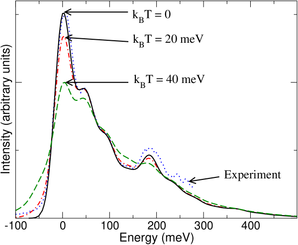
Figure 5: All-modes PES computed based on the effective-$A$ modes model at $k_{B}T$=$20$ and $40$ meV, for the couplings of Ref. 1, obtained through a $T=0$ fit to the PES data, and compared to experiment.

References

- [1] O. Gunnarsson, H. Handschuh, P. S. Bechthold, B. Kessler, G. Ganteför, and W. Eberhardt, Phys. Rev. Lett. 74, 1875 (1995); O. Gunnarsson, Phys. Rev. B 51, 3493 (1995).
- [2] C. M. Varma, J. Zaanen, and K. Raghavachari, Science 254, 989 (1991).
- [3] M. Schlüter, M. Lannoo, M. Needels, G. A. Baraff, and D. Tománek, Phys. Rev. Lett. 68, 526 (1991); J. Phys. Chem. Solids 53, 1473 (1992).
- [4] V. P. Antropov, O. Gunnarsson, and A. I. Lichtenstein, Phys. Rev. B 48, 7651 (1993).
- [5] N. Manini, A. Dal Corso, M. Fabrizio, and E. Tosatti, Philos. Mag. B 81, 793 (2001).
- [6] M. C. M. O’Brien, Phys. Rev. 187, 407 (1969).
- [7] A. Auerbach, N. Manini, and E. Tosatti, Phys. Rev. B 49, 12998 (1994).
- [8] N. Manini and P. De Los Rios, Phys. Rev. B 62, 29 (2000).
- [9] P. H. Butler, Point Group Symmetry Applications (Plenum, New York, 1981).
- [10] P. Brühwiler, A. J. Maxwell, P. Balzer, S. Andersson, D. Arvanitis, L. Karlsson, and N. Mårtensson, Chem. Phys. Lett. 279, 85 (1997).
- [11] N. Manini, P. Gattari, and E. Tosatti, Phys. Rev. Lett. 91, 196402 (2003).
- [12] P. Gattari, Diploma thesis, http://www.mi.infm.it/manini/theses/gattari.pdf .
- [13] M. C. M. O’Brien, J. Phys. C 5, 2045 (1972).
- [14] N. Manini and E. Tosatti, Phys. Rev. B 58, 782 (1998).