Elastic Behavior of a Two-dimensional Crystal near Melting

Abstract

Using positional data from video-microscopy we determine the elastic moduli of two-dimensional colloidal crystals as a function of temperature. The moduli are extracted from the wave-vector-dependent normal mode spring constants in the limit $q\to 0$ and are compared to the renormalized Young’s modulus of the KTHNY theory. An essential element of this theory is the universal prediction that Young’s modulus must approach $16\pi$ at the melting temperature. This is indeed observed in our experiment.

In the early 70th Kosterlitz and Thouless Kosterlitz73 developed a theory of melting for two-dimensional systems. In their model the phase transition from a system with quasi-long-range order mermin is mediated by the unbinding of topological defects like vortices or dislocation pairs in the case of 2D crystals. They showed that the phase with higher symmetry has short-range translational order. Halperin and Nelson Halperin78 ; nelson79 pointed out that this phase still exhibits quasi-long-range orientational order and proposed a second phase transition now mediated by the unbinding of disclinations to an isotropic liquid. The intermediate phase is called hexatic phase. This theory, being based also on the work of Young Young79 , is known as KTHNY theory (Kosterlitz, Thouless, Halperin, Nelson and Young); it describes the temperature-dependent behavior of the elastic constants, the correlation lengths, the specific heat and the structure factor (for a review see Strandburg88 ; Glaser93 ). Experiments with electrons on helium Grimes79 ; Morf79 and with 2D interfacial colloidal systems Pieranski80 ; Murray87 ; Kusner94 ; Marcus97 ; zahn99 as well as computer simulations Chen95 ; Bagchi96 ; Jaster98 have been performed to test the essential elements of this theory. But research has mainly focused on the behavior of the correlation functions (an illustrative example is the work of Murray and van Winkle Murray87 ). Only a few works can be found that deal with the elastic constants, especially the shear modulus, Morf79 ; Fisher82 ; Morales94 ; Sengupta00 even though the Lam$\acute{e}$ coefficients and their renormalization near melting take a central place in the KTHNY theory.

A very strong prediction of the KTHNY theory has never been verified experimentally. It states that the renormalized Young’s Modulus $K_{R}(T)$, being related just to the renormalized Lam$\acute{e}$ coefficients $\overline{\mu}_{R}$ and $\overline{\lambda}_{R}$, must approach the value $16\pi$ at the melting temperature nelson79 ,

$$K_{R}(T)=4\overline{\mu}_{R}(1-\overline{\mu}_{R}/(2\overline{\mu}_{R}+\overline{\lambda}_{R}))\to 16\pi\quad\mbox{if}\>T\to T_{m}^{-}\>,$$ (1)

which is obviously an universal property of 2D systems at the melting transition. This Letter presents experimental data for elastic moduli of a two-dimensional colloidal model system, ranging from deep in the crystalline phase via the hexatic to the fluid phase. These data, indeed, confirm the theoretical prediction expressed by eq. (1).

The experimental setup is the same as already described in keim04 . The system is known to be an almost perfect 2D system; it has been successfully tested, and explored in great detail, in a number of studies zahn99 ; zahn97 ; zahn00 ; keim04 . Therefore we only briefly summarize the essentials here: Spherical colloids (diameter $d=4.5\>\mu m$) are confined by gravity to a water/air interface formed by a water drop suspended by surface tension in a top sealed cylindrical hole of a glass plate. The flatness of the interface can be controlled within $\pm$ half a micron. The field of view was $835\times 620\>\mu m^{2}$ containing typically up to $3\cdot 10^{3}$ particles (the whole system has a size of $50~{}mm^{2}$ and contains about $3\cdot 10^{5}$ particles). The particles are super-paramagnetic, so a magnetic field $\vec{B}$ applied perpendicular to the air/water interface induces in each particle a magnetic moment $\vec{M}=\chi\vec{B}$ which leads to a repulsive dipole-dipole pair-interaction energy of $\beta v(r)=\Gamma/(\sqrt{\pi\rho}r)^{3}$ with the dimensionless interaction strength given by $\Gamma=\beta(\mu_{0}/4\pi)(\chi B)^{2}(\pi\rho)^{3/2}$ ($\beta=1/kT$ inverse temperature, $\chi$ susceptibility, $\rho$ area density). The interaction can be externally controlled by means of the magnetic field $B$. $\Gamma$ was determined as in Ref. zahn99 and is the only parameter controlling the phase-behavior of the system. It may be considered as an inverse reduced temperature, $T=1/\Gamma$. For $\Gamma>\Gamma_{m}=60$ the sample is a hexagonal crystal zahn99 ; zahn00 . Coordinates of all particles at equal time steps and for different ’temperatures’, i.e. $\Gamma$’s, were recorded using digital video-microscopy and evaluated with an image-processing software. We measured over 2-3 hours and recorded trajectories of about 2000 particles in up to 3600 configurations, for a large number of different $\Gamma$’s ranging between $\Gamma=49$, deep in the fluid phase, to $\Gamma=175$ in the solid phase. These trajectories were then further processed to compute the elastic constants of the colloidal crystal as a function of the inverse temperature $\Gamma$.

Our data analysis is based on the classical paper of Nelson and Halperin (NH) on dislocation-mediated melting in 2D systems nelson79 . Their considerations start from the reduced elastic Hamiltonian,

$$\beta{\cal H}_{E}=\frac{1}{2}\int\frac{d^{2}r}{a^{2}}\big{[}2\overline{\mu}u_{ij}^{2}+\overline{\lambda}u_{kk}^{2}\big{]}$$ (2)

where $a$ is the lattice constant of a triangular lattice (next neighbor distance), while $\overline{\mu}=\mu a^{2}/kT$ and $\overline{\lambda}=\lambda a^{2}/kT$ denote the dimensionless Lam$\acute{e}$ coefficients ($\beta=1/kT$). $u_{ij}(\vec{r})=(\partial_{r_{j}}u_{i}(\vec{r})+\partial_{r_{i}}u_{j}(\vec{r}))/2$ is the usual strain tensor related to the displacement field $\vec{u}(\vec{r})$. At temperatures $T$ near the melting temperature $T_{m}$ the field $u_{ij}(\vec{r})$ contains singular parts $u^{sing}_{ij}(\vec{r})$ due to dislocations; it can be decomposed into $u_{ij}(\vec{r})=u^{sing}_{ij}(\vec{r})+\phi_{ij}(\vec{r})$ with $\phi_{ij}(\vec{r})=(\partial_{r_{j}}\phi_{i}(\vec{r})+\partial_{r_{i}}\phi_{j}(\vec{r}))/2$ being a smoothly varying function ($\vec{\phi}(\vec{r})$ is the regular part of the displacement field $\vec{u}(\vec{r})$). When this decomposition is inserted in eq. (2), the Hamiltonian decomposes into two parts, $\beta{\cal H}_{E}=1/2\int d^{2}r/a^{2}(2\overline{\mu}\phi_{ij}^{2}+\overline{\lambda}\phi_{kk}^{2})+\beta{\cal H}_{D}$ with ${\cal H}_{D}$ representing the extra elastic energy that is due to the dislocations. NH were able to derive a set of differential equations for renormalized Lam$\acute{e}$ coefficients, $\overline{\mu}_{R}$ $\overline{\lambda}_{R}$, by means of which ${\cal H}_{E}$ can again be written as in eq. (2),

$$\beta{\cal H}_{E}=\frac{1}{2}\int\frac{d^{2}r}{a^{2}}\big{[}2\overline{\mu}_{R}u_{ij}^{2}+\overline{\lambda}_{R}u_{kk}^{2}\big{]}\>.$$ (3)

Because the effect of the dislocations are entirely absorbed into the elastic constants, the strain tensor in eq. (3) can now be assumed to be again regular everywhere and for all $T<T_{m}$.

Our experiment measures the trajectories $\vec{r}_{i}(t)$ of $N$ particles of a colloidal crystal over a finite time window of width $t_{exp}$. Associating the average $\langle\vec{r}_{i}\rangle_{t_{exp}}$ with a lattice site $\vec{R}_{i}$, we can, for each particle, compute displacement vectors $\vec{u}(\vec{R}_{i})=\vec{r}_{i}-\vec{R}_{i}$ . The Fourier transforms of these displacement vectors, $\vec{u}(\vec{q})=N^{-1/2}\sum_{\vec{R}}e^{i\vec{q}\vec{R}}\vec{u}(\vec{R})$, are now used for the numerical computation of renormalized elastic constants. This has been done in the following way. Starting from eq. (3.29) of the NH paper,

$$\lim_{\vec{q}\to 0}q^{2}\langle u^{\ast}_{i}(\vec{q})u_{j}(\vec{q})\rangle=\frac{kT}{v_{0}}\Big{[}\frac{1}{\mu_{R}}\delta_{ij}-\frac{\mu_{R}+\lambda_{R}}{\mu_{R}(2\mu_{R}+\lambda_{R})}\frac{q_{i}q_{j}}{q^{2}}\Big{]}$$ (4)

we find, after decomposing the displacement field $\vec{u}(\vec{q})$ into parts $\vec{u}_{||}(\vec{q})$ and $\vec{u}_{\bot}(\vec{q})$, parallel and perpendicular to $\vec{q}$, that

$$\frac{v_{0}(2\mu_{R}+\lambda_{R})}{kT} = \lim_{\vec{q}\to 0}\zeta_{||}(\vec{q}),\>\>\zeta_{||}(\vec{q}):=\big{(}q^{2}\langle|u_{||}(\vec{q})|^{2}\rangle\big{)}^{-1}$$ (5)

$$\frac{v_{0}\mu_{R}}{kT} = \lim_{\vec{q}\to 0}\zeta_{\bot}(\vec{q}),\>\>\zeta_{\bot}(\vec{q}):=\big{(}q^{2}\langle|u_{\bot}(\vec{q})|^{2}\rangle\big{)}^{-1}$$ (6)

where $v_{0}=\sqrt{3}a^{2}/2$ is the area per colloid in a triangular lattice.

These two equations are the central equations for our data evaluation scheme, and are therefore more carefully discussed. Deep in the solid phase $\langle\vec{r}\rangle_{\Delta t}$ converges with increasing measurement time $\Delta t$ to lattice sites, and $\langle|\vec{u}(\vec{R})|^{2}\rangle$ and $(q^{2}\langle|\vec{u}(\vec{q})|^{2}\rangle)_{q\to 0}$ remain finite, and lead thus to two non-zero elastic moduli: the shear modulus $\mu$ and the bulk modulus $B=\lambda+\mu$. By contrast, in the fluid phase $\langle\vec{r}\rangle_{\Delta t}$ will neither converge to, nor correlate with, any sort of lattice site and, in addition, as the mean square displacement is unbound, $(q^{2}\langle|\vec{u}(\vec{q})|^{2}\rangle)_{q\to 0}\to\infty$, so, both moduli will vanish (while $B$ survives foot37HN ).

Though reasonable at first glance, this interpretation of eqs. (5,6) is in fact an oversimplification and ignores the limited applicability of both equations. This can best be seen by re-deriving them, first by Fourier-transforming eq. (3), by then inserting the decomposition $\vec{u}=\vec{u}_{||}+\vec{u}_{\bot}$ and by applying finally the equipartition theorem. The intimate relationship between eq. (3) and eqs. (5,6) let us realize that the $\vec{u}(\vec{q})$ in eqs. (5,6) refer to a coarse-grained and thus regular displacement field, just as in eq. (3). In other words, with eqs. (5,6) the softening of the elastic constants for $T\to T_{m}^{-}$ is inferred indirectly, namely from the change of behavior of the regular parts of a coarse-grained displacement field.

We here identify this coarse-grained displacement field with the $\vec{u}(\vec{r}(t))=\langle\vec{r}\rangle_{t_{exp}}-\vec{r}(t)$ evaluated from our experimental data. In doing so, we have to be aware of the following two points. (i) In an imperfect crystal, especially in the presence of dislocations, $\langle\vec{r}\rangle_{t_{exp}\to\infty}$ does not always converge to lattice sites. As we are interested in the limit $q\to 0$, this is unproblematic, as long as these extra sites do not move. Looking at our measured trajectories, we have observed only thermally activated dislocation pairs, but no static, isolated dislocations traveling through the crystal. (ii) The displacement field computed from the experimental data has (and must have) parts stemming from dislocations. The resulting error should be small below $T_{m}$ when the number of dislocations is still relatively low (even at $T=T_{m}$, the probability that a particle belongs to a dislocation is only 1 % !). However, the error should become appreciable at $T>T_{m}$ where eqs. (5,6) can not be expected to strictly hold any longer.

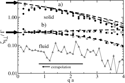
Figure 1: $\zeta_{||}(\vec{q})/\Gamma$ in a) and $\zeta_{\bot}(\vec{q})/\Gamma$ in b), as defined in eqs. (5,6). Each quantity is plotted for two different directions in $q$-space ($\Gamma\to M$ and $\Gamma\to K$ in the first Brillouin zone), and for three different values of the interaction-strength parameter $\Gamma$: $\Gamma=52$ in the fluid phase (open triangles), $\Gamma=75$ (open squares), and $\Gamma=125$ (filled circles) in the crystalline phase. Thick solid arrows for a $T=0$ prediction of the elastic moduli, dashed solid lines for the predictions of harmonic crystal theory. For $\Gamma=52$ just one band is shown.

For the pair-potential $\sim\Gamma/r^{3}$ the elastic constants can be calculated in the limit $\Gamma\to\infty$ ($T=0$) using simple thermodynamical relations involving essentially lattice sums of the pair-potential. One finds $\overline{\lambda}+\overline{\mu}=3.46\>\Gamma$ and $\overline{\mu}=0.346\>\Gamma$ wille . For convenience, we divide in the following all moduli by $\Gamma$. Fig. (1) shows $(\lambda+2\mu)v_{0}/\Gamma kT$ and $\mu v_{0}/\Gamma kT$, obtained from this $T=0$ calculation, as thick solid arrows, and compares it to the expressions $\zeta_{||}(\vec{q})/\Gamma$ and $\zeta_{\bot}(\vec{q})/\Gamma$ from eqs. (5,6), as obtained from the measured trajectories for three different values of $\Gamma$. Let us first focus on the measurement for $\Gamma=75,125$ where the system is deep enough in the crystalline phase for the assumption $T=0$ to be valid. $\zeta_{||}(\vec{q})/\Gamma$ and $\zeta_{\bot}(\vec{q})/\Gamma$, indeed, tend to the predicted elastic constants in the limit $q\to 0$, in agreement with eqs. (5,6). For either of the two plotted quantities, we consider two different high-symmetry directions in $q$ space, which are $\vec{q}_{1}=q\vec{b}_{1}$ and $\vec{q}_{2}=q(\vec{b}_{1}+\vec{b}_{2})/\sqrt{2}$ where $\vec{b}_{1}=(1,0)a$ and $\vec{b}_{2}=(1,\sqrt{3})a/2$ are basis vectors of the (hexagonal) reciprocal lattice. At wavelengths larger than the lattice constant ($qa<1$), the results for both bands are identical, thus indicating an essentially isotropic $\vec{u}(\vec{q})$ at small $q$. $\zeta_{||}(\vec{q})$ and $\zeta_{\bot}(\vec{q})$ can also be associated with the $\vec{q}$-dependent normal-mode spring constants (elastic dispersion curves) of the discrete crystal, having longitudinal $\lambda_{long}(\vec{q})$ and transversal $\lambda_{trans}(\vec{q})$ branches. This can be (and have been keim04 ) compared to the band-structure predicted by harmonic lattice theory (thick dashed lines in Fig. (1), for details see keim04 ). In other words, what we do here is to derive elastic constants from the $q\to 0$ behavior of the elastic dispersions curves ($\lim_{q\to 0}\lambda_{long}(\vec{q})=(\lambda+2\mu)q^{2}v_{0}$, $\lim_{q\to 0}\lambda_{trans}(\vec{q})=\mu q^{2}v_{0}$).

While for all our measurements above $\Gamma_{m}=60$ the resulting bands lie on top of the dashed thick lines in Fig. (1), one finds a systematic shift to smaller values for $\Gamma<\Gamma_{m}$. Fig. (1) shows, as an example, one out of the four bands (belonging to $\zeta_{\bot}(\vec{q})/\Gamma$) of the measurement in the fluid phase ($\Gamma=52$). It lies an order of magnitude below the crystalline bands.

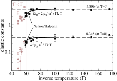
Figure 2: Elastic moduli of a 2D colloidal crystal as a function of the inverse temperature, obtained from extrapolating the bands in Fig. (1) down to $q=0$. The melting temperature is at $\Gamma_{m}=60$. Thick dashed lines for a $T=0$ prediction of the elastic moduli, $\overline{\lambda}+2\overline{\mu}=3.806\Gamma$ and $\overline{\mu}=0.346\Gamma$ wille ; thick solid line for the theoretical elastic constants, renormalized as described in nelson79 .

In order to infer functions $\mu_{R}(\Gamma)$ and $\lambda_{R}(\Gamma)$ from these bands, we need to take the limit $q\to 0$. Since at low $q$ we have to expect finite size effects, and at high $q$, near the edges of the first Brillouin zone, effects resulting from the band dispersion of the discrete lattice, we choose an intermediate $q$ regime ($0.8<qa<2.5$), indicated by the thick solid bar in Fig. (1), to extrapolate the bands to $q=0$, applying a linear regression scheme. The extrapolation procedure was optimized at high $\Gamma$ for which we have a precise idea what constants we should find. For each modulus, extrapolation of the two bands depicted in Fig. (1) were checked: while for $\zeta_{||}/\Gamma$, one finds for both bands the same modulus, the upper band of the two for $\zeta_{\bot}/\Gamma$ gave much better result and was henceforth taken. Also, different extrapolation schemes have been checked, but linear extrapolation turned out to produce a tolerably small error, much smaller than the main error of our measurement, estimated here from the standard error in the linear regression scheme.

Fig. (2) shows the resulting moduli, for all values of $\Gamma$ studied. Black symbols refer to systems in the crystalline state ($\Gamma>\Gamma_{m}$), grey data points to those in the fluid/hexatic phase. We postpone the discussion of the data points at $\Gamma<\Gamma_{m}$ and first concentrate on the crystalline regime where a renormalization of Lam$\acute{e}$ coefficients really makes sense. The thick dashed lines in Fig. (2) represent the $T=0$ calculation which holds down to $\Gamma$ values close to $\Gamma=75$. The thick solid line shows the theoretical curve for $\mu_{R}(\Gamma)$ and $\mu_{R}(\Gamma)+2\lambda_{R}(\Gamma)$, which we computed following the renormalization procedure outlined in the NH paper (Eq. (2.42),(2.43) and (2.45) in nelson79 with $K(\Gamma)=1.258\,\Gamma$ at $T=0$ and $\Gamma_{m}=60$ as input to set up the boundary conditions.) Theory and experiment agree well, considering that no fit parameter has been used. For $\Gamma>\Gamma_{m}$, all our results are converged, meaning that the computed moduli do not depend on the length of the trajectory. This is demonstrated by means of the $\Gamma=100$ measurement for which the moduli were computed taking only the first third of all configurations (open square symbol in Fig. (2)).

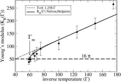
Figure 3: Young’s modulus, eq. (1), as a function of the inverse temperature, evaluated with the experimentally determined Lam$\acute{e}$ coefficients of Fig. (2) (symbols). The solid curve is $K_{R}(\Gamma)$ renormalized according to nelson79 , while the dashed curve is based on the T=0 prediction.

Fig. (3) now checks eq. (1), with $K_{R}(\Gamma)$ evaluated using the elastic moduli from Fig. (2). Using the theoretical values from the $T=0$ calculation, we obtain $K(\Gamma)=1.258\,\Gamma$, shown in Fig. (3) as dashed line. The thick solid line shows the theoretical curve for $K_{R}(\Gamma)$ which we computed with Lam$\acute{e}$ coefficients that were renormalized following the NH procedure explained above. The main result of this work is that the experimental data points closely follow the theoretical curve and indeed, they cross $16\pi$ at $\Gamma=\Gamma_{m}$ in excellent agreement with the predictions of NH. The length of the remaining error bars correlate with the total measurement time, and the $q$-range chosen in the extrapolation step.

The data points for $\Gamma<\Gamma_{m}$ in Fig. (1) and (2) should be treated with utmost caution. For the reasons given above, it is not clear to us whether or not eqs. (5,6) is at all meaningful outside the crystalline phase. But even if it were, we should be aware that the results will always depend on the measurement time. This is demonstrated for a system at $\Gamma=49$ for which the moduli were calculated taking again just a fraction of 1/3 of all configurations (open symbols in Fig. (2)). There is almost an order of magnitude difference to the data points based on all configurations, thus indicating the dependence of the moduli on the length of the analyzed trajectories. Physically, one could interpret this in terms of a frequency-dependent shear modulus which for non-zero $\omega\sim 1/t_{exp}$ is known to exist even in fluids.

To conclude, we have measured particle trajectories of a two-dimensional colloidal model system and computed elastic dispersion curves which at low $\vec{q}$ give access to the elastic constants. We thus measured $\mu_{R}$, $\lambda_{R}$ and Young’s modulus $K_{R}$ as a function of the inverse temperature $\Gamma$. All three quantities compare well with corresponding predictions of the KTNHY theory. Young’s modulus, in particular, tends to $16\pi$ when the crystal melts, as predicted in nelson79 .

We acknowledge stimulating discussions with Matthias Fuchs and David Nelson as well as financial support from the Deutsche Forschungsgemeinschaft (European Graduate College ’Soft Condensed Matter’ and Schwerpunktprogramm Ferrofluide, SPP 1104)

References

- (1) J. Kosterlitz and D. Thouless, J. Phys. C: Solid State Phys., 6, 1181 (1973).
- (2) N.D. Mermin, Phys. Rev. 176, 250, (1968); R..E. Peierls, Helv. Phys. 7, 81, (1923); L.D. Landau, Phys. Z. Sowjet, 11, 26, (1937).
- (3) B. Halperin and D. Nelson, Phys. Rev. Lett., 41, 121 (1978).
- (4) D.R. Nelson and B.I. Halperin, Phys. Rev. B, 19, 2457 (1979).
- (5) A. Young, Phys. Rev. B,19, 1855 (1979).
- (6) K. J. Strandburg, Rev. Mod. Phys., 60, 161 (1988).
- (7) M. Glaser and N. Clark, Adv. Chem. Phys., 83, 543 (1993).
- (8) C. Grimes and G. Adams, Phys. Rev. Lett., 42, 795 (1979).
- (9) R. Morf, Phys.Rev.Lett., 43, 931 (1979).
- (10) P. Pieranski,Phys. Rev. Lett., 45, 569 (1980).
- (11) C.A. Murray and D.H. Van Winkle, Phys. Rev. Lett., 58, 1200 (1987).
- (12) R. Kusner, J. Mann, J. Kerins, and A. Dahm, Phys. Rev. Lett. 73,3113 (1994).
- (13) A. Marcus and S. Rice, Phys. Rev. E, 55, 637 (1997).
- (14) K. Zahn, R. Lenke, and G. Maret, Phys. Rev. Lett. 82, 2721 (1999)
- (15) K. Chen, T. Kaplan, and M. Mostoller Phys. Rev. Lett., 74, 4019 (1995).
- (16) K. Bagchi and H. Andersen, Phys. Rev. Lett., 76, 255 (1996).
- (17) A. Jaster, Europhys. Lett., 42, 277 (1998).
- (18) D. Fisher, Phys. Rev. B, 26, 5009 (1982).
- (19) J. Morales, Phys. Rev. E 49, 5127 (1994).
- (20) S. Sengupta, P. Nielaba, M. Rao and K. Binder, Phys. Rev. E, 61, 1072 (2000);S. Sengupta, P. Nielaba and K. Binder Phys. Rev. E, 61, 6294 (2000).
- (21) K. Zahn, J.M.Mendez-Alcaraz and G. Maret, Phys. Rev. Lett 79, 175 (1997); K. Zahn, G. Maret, C. Ruß, and H.H. von Grünberg, Phys. Rev. Lett. 91, 115502 (2003); K. Zahn, A. Wille, G. Maret, S. Sengupta, and P. Nielaba, Phys. Rev. Lett. 90, 155506 (2003).
- (22) K. Zahn and G. Maret, Phys. Rev. Lett. 85, 3656 (2000).
- (23) P. Keim, G. Maret, U. Herz, and H.H. von Grünberg, Phys.Rev.Lett., 92,215504-1 (2004).
- (24) see footnote 37 of nelson79 .
- (25) A.Wille, Ph.D. thesis, University of Konstanz, Konstanz, Germany, (2001).