Lifetime of small systems controlled by autocatalytic reactions

Abstract

By using the point model of reaction kinetics we have studied the stochastic properties of the lifetime of small systems controlled by autocatalytic reaction $A+X\rightleftharpoons X+X,\;\;X\rightarrow B$. Assuming that a system is living only when the number of autocatalytic particles is larger than zero but smaller than a positive integer $N$, we have calculated the probability of the lifetime provided that the number of substrate particles $A$ is kept constant by a suitable reservoir, and the end-products $B$ do not take part in the reaction. We have shown that the density function of the lifetime is strongly asymmetric and in certain cases it has a well-defined minimum at the beginning of the process. It has been also proven that the extinction probability of systems of this type is exactly $1$.

I Introduction

Finding models for calculations of lifetime probability of systems evolving in accordance to well-defined rules seems to be a very attractive problem kendall50 ; bharucha53 ; eigen71 ; segre98 ; ferreira03 not only in physics but also in many other fields of sciences. The system evolution is usually controlled by stochastic transformations of components which are called in the sequel ”particles”. In the present model the transformation is realized by autocatalytic reactions which play important role in organization and coordination of systems having small spatial volume and containing few particles only.

In this paper we are dealing with small systems which are in living state when the number of autocatalytic particles remains within the interval $(0,N)$, where $N$ is a positive integer, while the number of substrate particles is kept constant by a suitable reservoir. One can say that both the absence and the large ”dose” of $X$ particles lead to the extinction of the system. We would like to determine the lifetime probability of such systems.

We choose from many possible autocatalytic reactions one of the simplest, namely $A+X\rightleftharpoons X+X,\;\;X\rightarrow B$, where $A$ denotes the substrate particles the number of which

Figure 1: Illustration of a reversible autocatalytic reaction by a simple graph.

is assumed to be constant, and $X$ symbolizes the autocatalytic particles. The end-product particles $B$ do not take part in the reaction. For the sake of descriptiveness the reaction $A+X\rightleftharpoons X+X$ is illustrated by a simple graph shown in FIG. 1, where the white circle corresponds to an autocatalytic while the black one to a substrate particle.

Figure 2: Illustration of a system transformation caused by autocatalytic reaction.

A system consisting of $N_{A}$ substrate and $N_{X}$ autocatalytic particles can be represented by a set of complete graphs $K_{N}$ on $V=N_{A}+N_{X}$ points, where $N_{A}$ is fixed and $\max N_{X}$ is denoted by $N$. A randomly chosen point of a graph may be either $A$ or $X$, the only requirement is that the total numbers of $A$ and $X$ points must be $N_{A}$ and $N_{X}$, respectively. Clearly, the number of complete graphs characterizing a given systems is given by $1/B(N_{A}+1,N_{X}+1)$, where $B(x,y)$ is the beta function. Since every two points adjacent, the possibility of the interaction between any two particles of the system is the same. Therefore, it is obvious that the point model of reaction kinetics introduced by lpal04 can be applied. As an example, FIG. 2 illustrates a transformation which brings about a system of $V=6$ particles from a system of $V=5$ particles and vice versa.

In Section II we derive equations determining the probability $p(t,n)$ of finding $n$ autocatalytic particles at the time moment $t$ in a system of volume $V$ provided that at $t=0$ the number of particles was $i$. In Section III we show that the extinction probability of the system is $1$, while in Section IV results of exact calculations for $N=3$ and $N=5$ are presented. The main conclusions are summarized in Section V.

II Systems with limited number of autocatalytic particles

Now, we formulate the basic equation. Let $\xi(t)$ be the number of autocatalytic particles $X$ at time instant $t\geq 0$ in a system open for substrate particles $A$. In the sequel, we would like to define a special system existing only when $\xi(t)$ remains within the interval $(0,N)$, where $N$ is a positive integer. We say the system is in the state ${\mathcal{S}}_{n}$, if $\xi(t)=n$. Obviously, a system will be annihilated when it enters into the state either ${\mathcal{S}}_{0}$ or ${\mathcal{S}}_{N}$. For the sake of simplicity we call a system of this type SL system.

In order to characterize the stochastic behavior of an SL system we define the transition probabilities 

$${\mathcal{P}}\{\xi(t)=n|\xi(0)=i\}=p_{i,n}(t)=p_{n}(t),\;\;\;\;\;\;n=0,1,2,\ldots,N,$$

which are determined by the following equations:

$$\frac{dp_{0}(t)}{dt}=\gamma p_{1}(t),$$ (1)

$$\frac{p_{n}(t)}{dt}=-n(N_{A}\alpha+n\beta-\beta+\gamma)p_{n}(t)+(n-1)N_{A}\alpha p_{n-1}(t)+(n+1)(n\beta+\gamma)p_{n+1}(t),$$ (2)

$$n=1,2,\ldots,N-2.$$

Since there is no way out from the state ${\mathcal{S}}_{N}$ the equation for $p_{N-1}(t)$ should have the form

$$\frac{p_{N-1}(t)}{dt}=-(N-1)(N_{A}\alpha+N\beta-2\beta+\gamma)p_{N-1}(t)+(N-2)N_{A}\alpha p_{N-2}(t),$$ (3)

and, finally the equation

$$\frac{p_{N}(t)}{dt}=(N-1)N_{A}\alpha p_{N-1}(t)$$ (4)

determines the probability of the transition ${\mathcal{S}}_{i}\rightarrow{\mathcal{S}}_{N}$ during the time $t\geq 0$. Introducing the vector

$$\vec{\bf p}(t,N-1)=\left(\begin{array}[]{c}p_{N-1}(t)\\ p_{2N-2}(t)\\ \vdots\\ p_{1}(t)\end{array}\right)$$

and the matrix

$${\bf A}_{N-1}=\begin{pmatrix}-D_{N-1}&B_{N-1}&0&0&\cdots&0&0&0\\ C_{N-2}&-D_{N-2}&B_{N-2}&0&\cdots&0&0&0\\ 0&C_{N-3}&-D_{N-3}&B_{N-3}&\cdots&0&0&0\\ \vdots&\vdots&\vdots&\vdots&\cdots&\vdots&\vdots&\vdots\\ 0&0&0&0&\cdots&C_{2}&-D_{2}&B_{2}\\ 0&0&0&0&\cdots&0&C_{1}&-D_{1}\end{pmatrix},$$ (5)

we can write Eqs. (2) and (3) in the following compact form:

$$\frac{d\vec{\bf p}(t,N-1)}{dt}=\beta{\bf A}_{N-1}\;\vec{\bf p}(t,N-1),$$ (6)

with initial conditions $p_{n}(0)=\delta_{n,i}\;\;\text{for}\;\;1\leq n\leq N-1$. The elements of the matrix $\mathbf{A}_{N-1}$ are given by

$$B_{n}=(n-1)a,\;\;\;\;\;\;D_{n}=n(a+b+n-1),\;\;\;\;\;\;\mbox{and}\;\;\;\;\;C_{n}=(n+1)(b+n),$$ (7)

$$1\leq n\leq N-1,$$

where

$$a=N_{A}\;\frac{\alpha}{\beta},\;\;\;\;\;\;\text{and}\;\;\;\;\;\;b=\frac{\gamma}{\beta}.$$ (8)

One has to note that for the complete description of the process we need also the equations (1) and (4). The matrix ${\bf A}_{N-1}$ is a normal Jacobi matrix. (See Ref. dean56 ; karlin58 ; bellman60 .) It can be proven that the eigenvalues of $\mathbf{A}_{N-1}$ are different, negative real numbers. The proof is given in Appendix A. Consequently we obtain

$$\lim_{t\rightarrow\infty}p_{n}(t)=0,\;\;\;\;\;\;\mbox{if}\;\;\;\;\;\;n=1,2,\ldots,N-1,$$

but

$$\lim_{t\rightarrow\infty}p_{0}(t)=w_{0},\;\;\;\;\;\;\lim_{t\rightarrow\infty}p_{N}(t)=w_{N}\;\;\;\;\;\;\mbox{and}\;\;\;\;\;\;w_{0}+w_{N}=1,$$ (9)

i.e. if $t\rightarrow\infty$, then an SL system can be found either in ${\mathcal{S}}_{0}$ or in ${\mathcal{S}}_{N}$ state.

III Lifetime probability

The random time $\theta_{i},\;1\leq i\leq N-1$ due to the transitions either ${\mathcal{S}}_{i}\rightarrow{\mathcal{S}}_{0}$ or ${\mathcal{S}}_{i}\rightarrow{\mathcal{S}}_{N}$ is called the lifetime of the SL system. In other words, the lifetime is a random time interval at the end of which the number of autocatalytic particles becomes either zero or $N$. Formulating more precisely we can write

$$\{\theta_{i}\leq t\}=\{\xi(t)=0|\xi(0)=i\}\cup\{\xi(t)=N|\xi(0)=i\}$$

and since $\{\xi(t)=0|\xi(0)=i\}\cap\{\xi(t)=N|\xi(0)=i\}=\emptyset$, we have

$${\mathcal{P}}\{\theta_{i}\leq t\}=H_{i}(t)=p_{i,0}(t)+p_{i,N}(t).$$ (10)

By using Eqs. (9) we see immediately that

$$\lim_{t\rightarrow\infty}H_{i}(t)=1,\;\;\;\;\;\;\forall\;1\leq i\leq N-1,$$ (11)

i.e. the probability that the lifetime of the system is finite is equal to $1$. 

IV Systems with small number of states

The mathematical properties of the equation (6) are well-known karlin57 . Here, we do not wish to make detailed analysis of Eq. (6) and do not derive its formal solution, but instead we try to study the basic properties of exact solutions in those cases when the maximal number of autocatalytic particles is $N=3$ and $N=5$, i.e. the number of states is four and six, respectively.

IV.1 Four states systems

In order to have an insight into the dynamics of the process producing random transitions between different states of the system we are dealing now with a very simple system having only four states, namely ${\mathcal{S}}_{0},\;{\mathcal{S}}_{1},\;{\mathcal{S}}_{2},$ and ${\mathcal{S}}_{3}$. In this case the equations to be solved are

$$\frac{dp_{0}(t)}{dt} = \gamma p_{1}(t),$$ (12)

$$\frac{dp_{1}(t)}{dt} = -(\alpha\;N_{A}+\gamma)\;p_{1}(t)+2\;(\beta+\gamma)\;p_{2}(t),$$ (13)

$$\frac{dp_{2}(t)}{dt} = \alpha\;N_{A}\;p_{1}(t)-2\;(\alpha\;N_{A}+\beta+\gamma)\;p_{2}(t),$$ (14)

$$\frac{dp_{3}(t)}{dt} = 2\;\alpha\;N_{A}\;p_{2}(t).$$ (15)

The initial conditions to be used are $p_{0}(0)=p_{2}(0)=p_{3}(0)=0$ and $p_{1}(0)=1$. Introducing the notations (8), after elementary calculations one obtains

$$p_{0}(t)=b\frac{d-a-b-2}{2d\;\omega_{1}}\;(1-\exp\{-\omega_{1}\beta t\})+b\frac{d+a+b+2}{2d\;\omega_{2}}\;(1-\exp\{-\omega_{2}\beta t\}),$$ (16)

$$p_{1}(t)=\frac{\exp\{-\omega_{2}\beta t\}+\exp\{-\omega_{1}\beta t\}}{2}+\frac{a+b+2}{2d}\;\left(\exp\{-\omega_{2}\beta t\}-\exp\{-\omega_{1}\beta t\}\right),$$ (17)

$$p_{2}(t)=\frac{a}{d}\left(\exp\{-\omega_{2}\beta t\}-\exp\{-\omega_{1}\beta t\}\right),$$ (18)

and

$$p_{3}(t)=2\;\frac{a^{2}}{d}\;\left(\frac{1-\exp\{-\omega_{2}\beta t\}}{\omega_{2}}-\frac{1-\exp\{-\omega_{1}\beta t\}}{\omega_{1}}\right),$$ (19)

where

$$d=\sqrt{a^{2}+(b+2)^{2}+2a(5b+6)},\;\;\;\;\;\;\omega_{1}=\frac{1}{2}(\lambda+d)\;\;\;\;\;\;\mbox{and}\;\;\;\;\;\;\omega_{2}=\frac{1}{2}(\lambda-d),$$ (20)

while

$$\lambda=2+3\;(a+b).$$ (21)

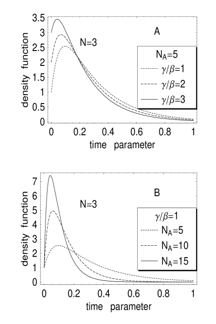
Figure 3: Probability density functions of the system lifetime $\theta_{1}$. Part A shows the density functions at different $\gamma/\beta$ values when $N_{A}=5$, while part B illustrates the effect of the variation of the number of $A$ particles at fixed $\gamma/\beta$ value. The ratio $\alpha/\beta=1$.

According to the theorem on eigenvalues nonnegative eigenvalue cannot be occurred, therefore $\lambda>d$. Naturally, this inequality can be simply proven for all positive $a$ and $b$ by using Eqs. (20) and (21). 

The probability density functions of the system lifetime $\theta_{1}$ are plotted on FIG. 3 at different values of the number of $A$ particles (part $B$ of the figure) and at different $\gamma/\beta$ ratios (part $A$ of the figure). It is remarkable that the density functions are strongly asymmetric, and the most probable lifetimes measured in $\beta^{-1}$ units are found near the zero of the time parameter.

As seen from Eqs. (12)-(15) we obtain the following limit probabilities:

$$\lim_{t\rightarrow\infty}p_{0}(t)=w_{0}=\frac{b\;(1+a+b)}{a^{2}+b\;(1+a+b)},\;\;\;\;\lim_{t\rightarrow\infty}p_{3}(t)=w_{3}=\frac{a^{2}}{a^{2}+b\;(1+a+b)},$$ (22)

and

$$\lim_{t\rightarrow\infty}p_{1}(t)=\lim_{t\rightarrow\infty}p_{2}(t)=0.$$

According to this, after elapsing sufficiently long (i.e. infinite) time, the system can be found almost surly in ”dead” state either with probability $w_{0}$ in the state ${\mathcal{S}}_{0}$ or with probability $w_{3}$ in the state ${\mathcal{S}}_{3}$. Obviously $w_{0}+w_{3}=1$.

IV.2 Six states systems

Now, we would like to see how the number of possible living states effects on the properties of the lifetime. If the number of states is six, i.e. $N=5$, then the system has four living and two dead states. According to the notation introduced earlier, the living states are ${\mathcal{S}}_{1},{\mathcal{S}}_{2},{\mathcal{S}}_{3},{\mathcal{S}}_{4}$, while the dead ones ${\mathcal{S}}_{0}$ and ${\mathcal{S}}_{5}$.

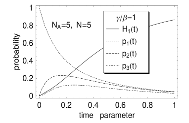
Figure 4: Dependence of probabilities $p_{1}(t),p_{2}(t),p_{3}(t)$ and the system lifetime distribution $H_{1}(t)$ on $t$ measured in $\beta^{-1}$ units. The ratio $\alpha/\beta=1$.

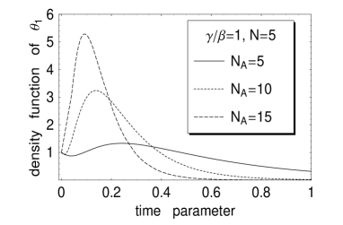
Figure 5: Density function of the system lifetime at different values of the number of $A$ particles at $\gamma/\beta=1$. The number of living states is equal to $4$. The time $t$ is measured in $\beta^{-1}$ units. The ratio $\alpha/\beta=1$.

By using numerical method for solving the equation system (1)-(4) in the case of $N=5$ we obtain the probabilities $p_{n}(t),\;n=0,1,\ldots,5$ vs. time parameter curves shown some of them in FIG. 4. What remarkable is the character of curves does not change with increasing number of possible states. It can be proven that the higher the number of possible states the larger is the probability that the system lifetime is longer than $t$.

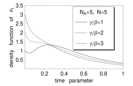
Figure 6: Density function of the system lifetime at different values of the ratio $\gamma/\beta$ and at the fixed number of $A$ particles. The number of living states is $4$ and the time $t$ is measured in $\beta^{-1}$ units. The ratio $\alpha/\beta=1$.

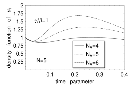
Figure 7: Density function of the system lifetime at the beginning of the process for three different values of the number of $A$ particles. The number of living states is $4$, the time $t$ is measured in $\beta^{-1}$ units and $\gamma/\beta=1$. The ratio $\alpha/\beta=1$.

Density functions of the system lifetime $\theta_{1}$ measured in $\beta^{-1}$ units are seen in FIG. 5 at values $N_{A}=5,10,15$. The calculations are performed at fixed $\gamma/\beta=1$ ratio. One can see the curves are strongly asymmetric and the most probable lifetime decreases with increasing $N_{A}$. The reason for this is clear: the speed of the reaction increases with the number of $A$ particles, and so if $N_{A}$ is large, then the state ${\mathcal{S}}_{N}$ can be reached in a time interval shorter than that is needed when $N_{A}$ is small. It is remarkable that we see in FIG. 6 showing the density function of $\theta_{1}$ at different $\gamma/\beta$ ratios. If the decay intensity $\gamma$ is approximately equal to the intensity $\beta$ of the reverse reaction $X+X\rightarrow X+A$, then a well-defined minimum appears in the density vs. lifetime curve at the very beginning of the process, because the autocatalytic production of $X$ particles cannot compensate the effect of the decay process. After elapsing some time the role of the autocatalytic process becomes perceptible and, if the ratio $\gamma/\beta$ is smaller than $3$, then the density function reaches a maximum which is followed by a monotonously decreasing part of the curve. The density function at the beginning of the process is shown in FIG. 7 for three $N_{A}$ values.

V Conclusions

Stochastic dynamics of small systema controlled by autocatalytic reaction $X+X\rightleftharpoons X+A,\;X\rightarrow B$ is studied. The dead state of systems is defined and the probability distribution of the lifetime are calculated by exact means. The density function of the lifetime is found to be strongly asymmetric (skewed right). The most probable lifetime (mode of the lifetime) decreases with increasing number of the substrate particles $A$. If the self-decay intensity of the autocatalytic particles is approximately equal to the intensity of the reverse reaction $X+X\rightarrow X+A$, then a well-defined minimum appears in the density function of the lifetime near the beginning of the process. It is remarkable that the basic character of the system’s dynamics does not vary significantly with increasing number of possible state.

Appendix A Eigenvalues

We would like to prove that the eigenvalues of the matrix $\mathbf{A}_{N-1}$ are different, negative real numbers. Let us introduce the matrix

$$\mathbf{J}_{n}=-\mathbf{A}_{n}=\begin{pmatrix}G_{n}&H_{n}&0&0&\cdots&0&0&0\\ F_{n-1}&G_{n-1}&H_{n-1}&0&\cdots&0&0&0\\ 0&F_{n-2}&G_{n-2}&H_{n-2}&\cdots&0&0&0\\ \vdots&\vdots&\vdots&\vdots&\cdots&\vdots&\vdots&\vdots\\ 0&0&0&0&\cdots&F_{2}&G_{2}&H_{2}\\ 0&0&0&0&\cdots&0&F_{1}&G_{1}\end{pmatrix},\;\;\;\;\;\;\text{where}\;\;\;\;\;\;n\in{\mathcal{Z}}_{+},$$ (23)

while

$$F_{j}=-(j+1)\;(b+j),\;\;\;\;\;\;G_{j}=j\;(a+b+j-1),\;\;\;\;\;\;H_{j}=-(j-1)\;a,$$ (24)

where $a$ and $b$ are positive real numbers given by Eq. (8). Since $F_{j}/H_{j-1}>0$ there is a diagonal matrix $\mathbf{S}_{n}$ such which transforms $\mathbf{J}_{n}$ into a symmetric matrix

$$\mathbf{R}_{n}=\mathbf{S}_{n}^{-1}\;\mathbf{J}_{n}\;\mathbf{S}_{n},$$ (25)

the eigenvalues of which are exactly the same as those of $\mathbf{J}_{n}$. The entries of $\mathbf{S}_{n}$ are

$$s_{i,j}=\delta_{i,j}\;s_{j},\;\;\;\;\;\;\text{where}\;\;\;\;\;\;s_{j}=\sqrt{\frac{F_{j}}{H_{j-1}}}\;s_{j-1},\;\;\;\;\;\;\text{and}\;\;\;\;\;\;s_{1}=1.$$

It is easy to show that

$$\mathbf{R}_{n}=\begin{pmatrix}G_{n}&\sqrt{H_{n}\;F_{n-1}}&0&0&\cdots&0&0&0\\ \sqrt{H_{n}\;F_{n-1}}&G_{n-1}&\sqrt{H_{n-1}\;F_{n-2}}&0&\cdots&0&0&0\\ 0&\sqrt{H_{n-1}\;F_{n-2}}&G_{n-2}&\sqrt{F_{n-3}\;H_{n-2}}&\cdots&0&0&0\\ \vdots&\vdots&\vdots&\vdots&\cdots&\vdots&\vdots&\vdots\\ 0&0&0&0&\cdots&\sqrt{F_{2}\;H_{3}}&G_{2}&\sqrt{F_{1}\;H_{2}}\\ 0&0&0&0&\cdots&0&\sqrt{F_{1}\;H_{2}}&G_{1}\end{pmatrix},$$ (26)

and clearly $\mathbf{R}_{n}$ is a symmetric Jacobi matrix. As known, if it is positive definite, then all of its eigenvalues are different, real and positive. A symmetric matrix is positive definite if the principal minors of the corresponding determinant are all positive. Let us denote by

$${\mathcal{D}}_{j}=\text{det}\;|\mathbf{R}_{j}|$$ (27)

the determinant due to the matrix $\mathbf{R}_{j}$. Taking into account that ${\mathcal{D}}_{0}=1$ by definition, we have to show that ${\mathcal{D}}_{j}>0,\;\;\forall\;j=1,2,\ldots,n$. After simple calculation we obtain

$${\mathcal{D}}_{j}=G_{j}\;{\mathcal{D}}_{j-1}-H_{j}\;F_{j-1}\;{\mathcal{D}}_{j-2},$$ (28)

and by induction we have

$${\mathcal{D}}_{j}=j!\sum_{i=0}^{j}\frac{\Gamma(b+i+1)}{\Gamma(b+1)}\;a^{j-i},$$ (29)

which clearly proves the statement. Finally, since the eigenvalues of $\mathbf{R}_{N-1}$ are real, positive and different, it follows that the eigenvalues of $\mathbf{A}_{N-1}$ are real, negative and different. Q.E.D.

References

- (1) D.G. Kendal, J. Roy. Statist. Soc., B 12, 278 (1950)
- (2) A.T. Bharucha-Reid, Biometrics, 9, 275 (1953)
- (3) M. Eigen, Naturwissenschaften, 58, 465 (1971)
- (4) D. Segré, Y. Pilpel, D. Lancet, Physica A, 249, 558 (1998)
- (5) A.S. Ferreira, M.A. da Silva, and J.C. Cressoni, Phys. Rev. Lett., 92, 219901-1 (2004)
- (6) L. Pál, arXiv:cond-mat/0404402
- (7) P. Dean, Proc. Cambridge Phil. Soc., 52, 752 (1956)
- (8) S. Karlin and J.L. McGregor, Techn. Rep., 9, Stanford University (1958)
- (9) R. Bellman, Introduction to matrix analysis, McGraw-Hill Book Company, INC. New York Toronto London (1960)
- (10) S. Karlin and J.L. McGregor, Trans. Amer. Math. Soc., 85, 489 (1957)