Spin systems with dimerized ground states

Abstract

In view of the numerous examples in the literature it is attempted to outline a theory of Heisenberg spin systems possessing dimerized ground states (“DGS systems") which comprises all known examples. Whereas classical DGS systems can be completely characterized, it was only possible to provide necessary or sufficient conditions for the quantum case. First, for all DGS systems the interaction between the dimers must be balanced in a certain sense. Moreover, one can identify four special classes of DGS systems: (i) Uniform pyramids, (ii) systems close to isolated dimer systems, (iii) classical DGS systems, and (iv), in the case of $s=1/2$, systems of two dimers satisfying four inequalities. Geometrically, the set of all DGS systems may be visualized as a convex cone in the linear space of all exchange constants. Hence one can generate new examples of DGS systems by positive linear combinations of examples from the above four classes.

1 Introduction

Spin systems with exact ground states are rare and hence have found considerable interest. A trivial case is a system of $N$ unconnected antiferromagnetic (AF) dimers which has the product $\Phi$ of the individual dimer ground states as its unique ground state. An interaction between the dimers would in general perturb the ground state, but, interestingly, for certain interactions $\Phi$ remains a ground state. In these cases the perturbational corrections of all orders will vanish; the interaction between the dimers is, so to speak, frozen for low temperatures.

Examples of these systems which minimize their energy for a product state $\Phi$ of dimer ground states (“DGS systems") have been constructed and studied in dozens of papers. Sometimes DGS systems are also referred to as “valence bond" (VB) systems, or, more generally, as “resonating valence bond" (RVB) systems if superpositions of VB states are involved. Here I can only mention a small selection of this literature. In the seminal papers of Majumdar and Ghosh [1][2] even $s=1/2$ rings are considered with constant NN and NNN interactions of relative strength $2:1$ which possess two different DGS according to the shift symmetry of the ring. More precisely, in the second of these papers [2] the authors proved as “an interesting by-product" that $\Phi$ is an eigenstate of the Hamiltonian and conjectured it being a ground state due to numerical studies up to 10 spins. One year later, Majumdar [3] mentions a proof of the DGS property for Majumdar-Ghosh rings given in a private communication by J. Pasupathy.

The generalization of these results to arbitrary spin quantum numbers $s$ is due to Shastry and Sutherland [4]. A different generalization of Majumdar-Ghosh rings has been given by Pimpinelli [5] and re-discovered by Kumar [6] who extended the coupling within the $s=1/2$ ring to $2n$-nearest neighbors with strengths $J_{1}=2n,J_{2}=2n-1,\ldots,J_{2n}=1$. Though it might not be adequate to call such a spin system still a “ring". Already the ring with NNN interaction could better be viewed as a “ladder". Ladders with DGS property have also been studied in [7] and [8]. Other one-dimensional models with DGS are certain dimer-plaquette chains, see [9] and [10].

Another family of two-dimensional DGS systems can be traced back to the work of Shastry and Sutherland [11] on square lattices with alternating diagonal bonds for every second square and arbitrary $s$. These authors also suggest to classify DGS states as a “spin liquids" due to their short range correlation. The S(hastry)S(utherland) model is physically realized in $SrCu_{2}(BO_{3})_{2}$, see [12] and [13].

Generalizations of the SS model are possible by introducing, additional to the nearest neighbor (NN) and diagonal (D) bonds, new types of interaction, namely next nearest neighbor (NNN), knight’s-move-distance-away (KM) and further-neighbor-diagonal (FND), see [14],[15] and [16]. The dimerized state $\Phi$ is then an eigenstate of the Hamiltonian if the five coupling constants involved satisfy

$$J_{1}:J_{2}:J_{3}:J_{4}:J_{5}=1:1:\frac{1}{2}:\frac{1}{2}:\frac{1}{4}\;.$$ (1)

If an inhomogeneous NN coupling is chosen, namely $J_{0}$ along the dimer bonds and $J_{1}$ for the remaining NN, the choice

$$J_{0}:J_{1}=7:1$$ (2)

yields a DGS for the generalized SS model, see [15].

Finally, I mention generalizations of the SS model to arbitrary dimensions [17] and by superpositions of uniform pyramids ($s=1/2$) constructed by Kumar [6] which will be reconsidered in section 3.1. For further related examples, see also [18].

In view of the abundance of examples of DGS systems in the literature I am not primarily interested in new examples but will try to characterize the class of all examples. Unfortunately, I have achieved a complete characterization only in the case of classical spin systems. This and the partial results for quantum systems are contained in sections 2 and 3. After the general definitions (subsection 2.1) a necessary condition is formulated (theorem 1 in subsection 2.2). It says that $\Phi$ will be an eigenstate of the spin Hamiltonian iff a certain balance condition for the four coupling constants between any two dimers is satisfied. For classical spin systems this balance condition can be strengthened to the condition of uniform coupling between any pair of dimers (theorem 2).

In section 3 I will give sufficient conditions for DGS systems and enumerate four special classes of examples. As mentioned above, systems of these classes can be superposed by positive linear combinations in order to form new DGS systems. Here we identify a spin system with its matrix ${\mathbb{J}}$ of exchange parameters and thus understand “addition" of systems as the addition of the corresponding matrices. Hence classical spin systems and quantum spin systems with any $s$ are not distinguished at the level of ${\mathbb{J}}$-matrices, but, of course, the definition of classical and quantum DGS systems is different.

Subsection 3.1 describes “uniform pyramids" which are systems of $N$ dimers with uniform coupling between all $2N$ spins (the base of the pyramid) plus an extra dimer one spin of which (the vertex of the pyramid) is uniformly coupled to the other $2N$ spins. These pyramids are DGS systems for arbitrary $s$ if the uniform coupling constants are suitably chosen. Another class of DGS systems is provided by small neighborhoods of unconnected dimer systems (subsection 3.2). The radius $r$ of the neighborhood decreases with $s$. Although $r$ is not the optimal value, there seems to be a trend that the class of DGS systems is shrinking if $s$ increases. This phenomenon can be illustrated by examples, see section 4, but has not yet been strictly proven.

For small $N$ and $s$ the class of DGS systems can, in principle, be explicitly determined. The method is sketched in subsection 3.3 and the result for $N=2,s=1/2$ is given in the form of four inequalities for polynomial functions of the involved four coupling constants. Recall that for a classical DGS system the coupling between any two pairs of dimers must be uniform. Hence it is possible to encode the structure of such a system by an $N\times N$ matrix ${\mathbb{G}}$ instead of the $2N\times 2N$ matrix ${\mathbb{J}}$. Then it can be shown that the system is a classical DGS system iff this matrix ${\mathbb{G}}$ is positive semi-definite, i. e. iff all its eigenvalues (or all its principal minors) are non-negative (theorem 3 in subsection 3.4). Moreover, if a coupling matrix ${\mathbb{J}}$ belongs to a classical DGS system, then it also belongs to a quantum DGS system for all values of $s$. Hence theorem 3 defines a forth class of special DGS systems.

In section 4 I will consider two examples. The first one (subsection 4.1) consists of two dimers which are weakly coupled in a balanced but not uniform way. If $\epsilon(s)$ is the maximal coupling strength such that the quantum system with spin quantum number $s$ is still DGS, then it follows that $\epsilon(s)\rightarrow 0$ for $s\rightarrow\infty$ since the classical system is not DGS for all $\epsilon>0$.

The second example (subsection 4.2) consists of three dimers and, due to symmetry assumptions, normalization and the balance condition, two independent coupling constants, say $J_{2}$ and $J_{4}$. It is still possible to exactly calculate the convex set of DGS systems in the $J_{2}-J_{4}-$plane and to illustrate the subsets defined in section 3 for this example.

For the sake of readability of the paper all proofs of the previously formulated theorems and propositions are deferred to section 5. In section 6 we investigate the geometric structure of the set ${\cal C}_{\Phi}$ of DGS systems, represented as the set of the corresponding ${\mathbb{J}}$-matrices. It is easily shown that ${\cal C}_{\Phi}$ is a proper, convex, generating cone in the linear space of all symmetric matrices satisfying the balance condition. Moreover, we will see that the interior points of ${\cal C}_{\Phi}$ are exactly those systems for which $\Phi$ is the unique ground state. Systems at the boundary of ${\cal C}_{\Phi}$ have degenerate ground states. In particular, the faces of ${\cal C}_{\Phi}$ consist of all DGS systems having the same eigenspace of ground states. We close with a summary (section 7).

2 Definitions and necessary conditions for DGS systems

2.1 Definitions

We consider systems of $2N$ spins with one and the same individual spin quantum number $s$ which are grouped into $N$ fixed pairs (“dimers"). To indicate this grouping the spins will be denoted by indices $\mu=(i,\delta)$ where $i=1,\ldots,N$ is the dimer index and $\delta=0,1$ distinguishes between the two spins belonging to the same dimer. Further we consider Heisenberg Hamiltonians

$$H({\mathbb{J}})=\sum_{\mu\nu}J_{\mu\nu}\bi{s}_{\mu}\cdot\bi{s}_{\nu}\;,$$ (3)

where $\bi{s}_{\mu}=(s_{\mu}^{(1)},s_{\mu}^{(2)},s_{\mu}^{(3)})$ denotes the $\mu$-th spin observable and ${\mathbb{J}}$ the $2N\times 2N$-matrix of real exchange parameters or coupling constants $J_{\mu\nu}$. All operators act on a $(2s+1)^{N}$-dimensional Hilbert space ${\cal H}=\bigotimes_{\mu=1}^{2N}{\cal H}_{\mu}$. If the spin quantum number $s$ is fixed, we may identify a spin system with its matrix ${\mathbb{J}}$.

Note that the exchange parameters $J_{\mu\nu}$ are not uniquely determined by the Hamiltonian $H({\mathbb{J}})$ via (3). Different choices of the $J_{\mu\nu}$ leading to the same $H({\mathbb{J}})$ will be referred to as different "gauges". We will adopt the following gauges: First, the antisymmetric part of ${\mathbb{J}}$ does not occur in the Hamiltonian (3). Hence we will follow common practice and choose $J_{\mu\nu}=J_{\nu\mu}$. Thus $\mathbb{J}$ is a real symmetric matrix . Second, since ${\bf s}_{\mu}\cdot{\bf s}_{\mu}=s(s+1)\;{\;\smash{\raisebox{-2.15277pt}{$\!\!\stackrel{{\scriptstyle\!\mbox{1}\rule[0.0pt]{0.18082pt}{4.82224pt}}}{{}}$}}}\;$ we may choose arbitrary diagonal elements $J_{\mu\mu}$ without changing $H({\mathbb{J}})$, as long as their sum vanishes, $\mbox{Tr}\;{\mathbb{J}}=0$. The usual gauge chosen throughout the literature is $J_{\mu\mu}=0,\;\mu=1,\ldots,N,$ which will be called the “zero gauge". In this article, however, we will choose the “homogeneous gauge", which is defined by the condition that the row sums will be independent of $\mu$, see also [19]:

$$j\equiv J_{\mu}\equiv\sum_{\nu}J_{\mu\nu}$$ (4)

Note that the eigenvalues of ${\mathbb{J}}$ may non–trivially depend on the gauge.

For any dimer with index $i$ let $[i0,i1]$ denote the ground state of the AF dimer $\bi{s}_{i0}\cdot\bi{s}_{i1}$ which is unique up to a phase and can be written in the form

$$[i0,i1]=\frac{1}{\sqrt{2s+1}}\sum_{m=-s}^{s}(-1)^{s-m}|m,-m\rangle\;,$$ (5)

using the eigenbasis $|m\rangle,\;m=-s,\ldots,s$ of $\bi{s}_{\mu}^{(3)}$. The ground state of a system of $N$ unconnected AF dimers is the product state

$$\Phi^{s}\equiv\bigotimes_{i=1}^{N}[i0,i1]\;,$$ (6)

called the dimerized state; it has the total spin quantum number $S=0$. A system ${\mathbb{J}}$ is said to admit dimerized ground states (DGS), or to have the DGS property, iff $\Phi^{s}$ is a ground state of $H({\mathbb{J}})$, i. e. iff

$$\langle\Phi^{s}|H({\mathbb{J}})\Phi^{s}\rangle\leq\langle\Psi|H({\mathbb{J}})\Psi\rangle$$ (7)

for all $\Psi\in{\cal H}$ with $||\Psi||=1$. Let ${\cal C}_{\Phi}^{s}$ denote the set of all spin systems ${\mathbb{J}}$ with the DGS property. If the quantum number $s$ is understood, we suppress it and write simply $\Phi$ and ${\cal C}_{\Phi}$.

Analogous definitions hold for the classical case: Here the spin observables $\bi{s}_{\mu}^{\small{cl}}$ are unit vectors, $H({\mathbb{J}})^{\small{cl}}$ is the Hamiltonian function, defined on the $2N$-fold Cartesian product of unit spheres

$${\cal P}\equiv{\begin{array}[]{c}{\scriptstyle N}\\ {\mbox{\Large\sf X}}\\ {}^{\scriptstyle\mu=1}\end{array}}{\cal S}_{(\mu)}^{2}\;,$$ (8)

and $\Phi^{\small{cl}}\subset{\cal P}$ is the set of all spin configurations satisfying

$$\bi{s}_{i0}+\bi{s}_{i1}=\bi{0}\;\mbox{ for all }i=1,\ldots,N\;.$$ (9)

Note that $\Phi^{\small{cl}}$ as well as $\Phi^{\small{s}}$ are invariant under rotations. ${\mathbb{J}}$ is said to have the classical DGS property iff the minimum of $H({\mathbb{J}})$ is assumed for all $\bi{s}\in\Phi^{\small{cl}}$. In this case we write ${\mathbb{J}}\in{\cal C}_{\Phi}^{\small{cl}}={\cal C}_{\Phi}^{\infty}$.

2.2 Necessary conditions for DGS systems

Whereas a complete characterization of ${\cal C}_{\Phi}^{s}$ seems to be possible only for small $N$ and $s$ or for the classical case $s=\infty$, one can prove a number of partial results, either necessary or sufficient conditions for ${\mathbb{J}}\in{\cal C}_{\Phi}^{s}$.

Necessary conditions of a rather trivial kind can be obtained whenever one finds a state $\Psi\in{\cal H}$ such that the r. h. s. of (7) can be explicitely calculated. Less trivial is the following

Theorem 1

$\Phi$ is an eigenstate of $H({\mathbb{J}})$ iff

$$J_{i0,j0}+J_{i1,j1}=J_{i0,j1}+J_{i1,j0}$$ (10)

for all $i<j=2,\ldots,N$.

This theorem says that for a DGS system the interaction between any pair of dimers has to be balanced in a certain sense: The strength of the inter-dimer parallel bonds must equal the strength of the diagonal bonds, but the strength of the dimer bonds may be arbitrary. For example, a spin square is never DGS because there are no diagonal bonds at all.
To give another example, is easy to derive from theorem 1 the condition (1) for $\Phi$ being an eigenstate of the generalized SS model by superposing five suitable dimer pairs of the square lattice, see figure 1.

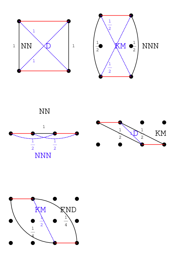
Figure 1: Decomposition of the generalized SS model [14] [15] [16] into pairs of dimers satisfying (10). The types of interaction are explained in the Introduction

If $\Phi$ is an eigenstate of $H({\mathbb{J}})$, it is straight forward to calculate the corresponding eigenvalue, since $\langle\Phi|\bi{s}_{i\delta}\cdot\bi{s}_{j\epsilon}|\Phi\rangle=0$ for $i\neq j$, see section .

Corollary 1

If $\Phi$ is an eigenstate of $H({\mathbb{J}})$, then

$$H({\mathbb{J}})\Phi=-2s(s+1)\sum_{i=1}^{N}J_{i0,i1}\;\Phi\;.$$ (11)

Because (10) is a linear equation, the set of all real, symmetric, traceless $2N\times 2N$-matrices ${\mathbb{J}}$ satisfying (4) and (10) will be a linear space of dimension $\frac{1}{2}N(3N-1)$, denoted by ${\cal J}_{\Phi}$. Further note that the ground state condition (7) is conserved under positive linear combinations of ${\mathbb{J}}$’s. Hence the set ${\cal C}_{\Phi}$ of DGS systems will form a convex cone embedded in the linear space ${\cal J}_{\Phi}$. Further geometrical properties of ${\cal C}_{\Phi}$ will be discussed in section 6.

Another necessary condition for the DGS property is the following:

Proposition 1

If ${\mathbb{J}}\in{\cal C}_{\Phi}$ then $J_{i0,i1}\geq 0$ for all $i=1,\ldots,N$.

Note, however, that the coupling between the dimers can be negative and nevertheless the system may have a DGS. For example, this may happen for systems close to unconnected dimer systems, see proposition 3.

In the classical case we have similar but stronger results: The balance condition (10) can be strengthened to a uniform coupling condition:

Theorem 2

If ${\mathbb{J}}\in{\cal C}_{\Phi}^{\small{cl}}$ then

$$J_{i0,j0}=J_{i0,j1}=J_{i1,j0}=J_{i1,j1}\equiv\epsilon_{ij}$$ (12)

and

$$J_{i0,i1}\geq 0$$ (13)

for all $i<j=2,\ldots,N$.

Consequently, we will denote by ${\cal J}_{\Phi}^{\infty}\equiv{\cal J}_{\Phi}^{\small{cl}}$ the linear space of all real, symmetric, traceless $2N\times 2N$-matrices ${\mathbb{J}}$ satisfying (4) and (12).

3 Sufficient conditions for DGS systems

We consider four classes of DGS systems which will hopefully cover all examples known from the literature by means of positive linear combinations of ${\mathbb{J}}$-matrices. Note that also DGS systems with a different number of dimers can be superposed in this sense.

3.1 Uniform pyramids

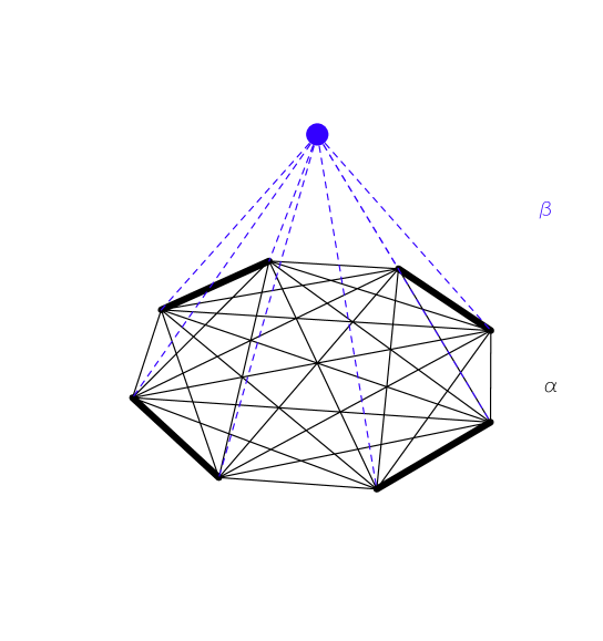
Figure 2: The uniform pyramid is a DGS system if $\alpha,\beta$ satisfy (16).

A uniform pyramid consists of $N$ dimers with uniform coupling between all $2N$ spins plus another uniform coupling with one extra spin, see figure 2. This extra spin with indices $(N+1,0)$ is considered as a part of another $N+1$-th dimer, in order to make it possible to define the dimerized state $\Phi$. More precisely, we require

$$J_{i\delta,j\epsilon} = \alpha>0\mbox{ for all }i,j=1,\ldots,N\mbox{ and }\delta,\epsilon\in\{0,1\}$$

$$\mbox{ except for }(i,\delta)=(j,\epsilon)\;,$$

$$J_{i\delta,N+1\;0} = \beta>0\mbox{ for all }i=1,\ldots,N\mbox{ and }\delta\in\{0,1\}$$ (15)

Then the following holds:

Proposition 2

Let ${\mathbb{J}}$ be a uniform pyramid such that

$$\frac{\beta}{\alpha}\leq\left\{\begin{array}[]{cll}\frac{1}{s+1}&\mbox{if}&s>\frac{1}{2}\\ 1&\mbox{if}&s=\frac{1}{2}\;.\end{array}\right.$$ (16)

Then ${\mathbb{J}}\in{\cal C}_{\Phi}$ .

DGS systems generated by uniform pyramids for $s=1/2$ have been considered by Kumar [K]. The $s=1/2$ Majumdar-Ghosh ring [2] can be viewed as a superposition of $N$ uniform triangles, similarly the SS model [11].

A superposition of uniform pyramids always yields DGS systems with $J_{\mu\nu}\geq 0$. But this condition is not necessary, as can be seen by the next class of DGS systems.

3.2 Neighborhoods of unconnected dimer systems

For matrices ${\mathbb{J}}\in{\cal C}_{\Phi}$ we define its spin modulus

$${\cal x}({\mathbb{J}})\equiv|j_{\small{min}}|$$ (17)

as the absolute value of the lowest eigenvalue $j_{\small{min}}$ of ${\mathbb{J}}$. It has similar properties as a matrix norm. For example, $j_{\small{min}}=0$ implies that all eigenvalues of ${\mathbb{J}}$ vanish, since $\mbox{Tr }{\mathbb{J}}=0$, and hence ${\mathbb{J}}=0$. But since, in general, ${\cal x}(-{\mathbb{J}})\neq{\cal x}({\mathbb{J}})$, the spin modulus will not be a norm. Nevertheless it can be used to define neighborhoods of matrices ${\mathbb{J}}\in{\cal C}_{\Phi}$ because it can easily be shown that

$$\frac{1}{2N-1}\|{\mathbb{J}}\|\leq{\cal x}({\mathbb{J}})\leq\|{\mathbb{J}}\|$$ (18)

holds, where $\|{\mathbb{J}}\|\equiv\max\{\;\|{\mathbb{J}}x\|\;|\;\|x\|=1\;\}$ denotes the so-called spectral norm, see [Lancaster69].

Let $\stackrel{{\scriptstyle\circ}}{{\mathbb{J}}}$ denote the matrix of an unconnected AF dimer system, i. e. $\stackrel{{\scriptstyle\circ}}{{J}}_{i0,i1}>0$ for all $i=1,\ldots,N$ and all other non-diagonal matrix elements vanish. Of course, $\stackrel{{\scriptstyle\circ}}{{\mathbb{J}}}\in{\cal C}_{\Phi}$. But also a small neighborhood of $\stackrel{{\scriptstyle\circ}}{{\mathbb{J}}}$ still consists of DGS systems. More precisely:

Proposition 3

Let $\stackrel{{\scriptstyle\circ}}{{\mathbb{J}}}$ be an unconnected dimer system and $\lambda=\min\{J_{i0,i1}|i=1\ldots N\}$. Further let ${\mathbb{J}}=\stackrel{{\scriptstyle\circ}}{{\mathbb{J}}}+\Delta,\;\Delta\in{\cal J}_{\Phi}$ such that

$${\cal x}(\Delta)\leq\frac{\lambda}{Ns(s+1)}\;.$$ (19)

Then ${\mathbb{J}}\in{\cal C}_{\Phi}$.

This proposition implies that the cone ${\cal C}_{\Phi}$ generates ${\cal J}_{\Phi}$, i. e. ${\cal J}_{\Phi}={\cal C}_{\Phi}-{\cal C}_{\Phi}$. Hence it is not possible to find a smaller subspace of ${\cal J}_{\Phi}$ which already contains all DGS systems. This stands in contrast to the classical case, see theorem 2. Moreover, the $s$-dependence of the bound in (19) supports the conjecture that the cones ${\cal C}_{\Phi}^{s}$ shrink with increasing $s$.

3.3 The case $s=1/2$

In principle, the cone ${\cal C}_{\Phi}$ could be exactly determined as follows: Calculate the characteristic polynomial $p(\lambda)=\det(H({\mathbb{J}})-\lambda\;\;\smash{\raisebox{-2.15277pt}{$\!\!\stackrel{{\scriptstyle\!\mbox{1}\rule[0.0pt]{0.18082pt}{4.82224pt}}}{{}}$}})$ of $H({\mathbb{J}}),\;{\mathbb{J}}\in{\cal J}_{\Phi}$. Its roots are the real eigenvalues $E_{\nu}$ of $H({\mathbb{J}})$; one of them, say $E_{0}$, will be the eigenvalue of $H({\mathbb{J}})$ w. r. t. $\Phi$. Factor $p(\lambda)=q(\lambda)(\lambda-E_{0})$. Then ${\mathbb{J}}\in{\cal C}_{\Phi}$ is equivalent to the condition that $E_{0}\leq$ any root of $q(\lambda)$. One can easily find criteria for this inequality which do not assume that the roots of $q(\lambda)$ are known. Consider, for example, the simple case of $q$ being quadratic, say $q(\lambda)=(\lambda-a)(\lambda-b),\;a<b$. Then obviously $E_{0}\leq a$ iff $q(E_{0})\geq 0$ and $q^{\prime}(E_{0})\leq 0$. More generally, one can prove the following:

Lemma 1

Let $q(\lambda)=\sum_{\ell=0}^{K}a_{\ell}\lambda^{\ell},\;a_{K}>0,$ have only real roots. Then $E_{0}\leq$ any root of $q(\lambda)$ iff

$$(-1)^{K+n}q^{(n)}(E_{0})\geq 0\mbox{ for all }n=0,\ldots,K-1\;.$$ (20)

Thus it is possible to explicitely determine ${\cal C}_{\Phi}$ by $K=(2s+1)^{2N}-1$ inequalities without calculating the $E_{\nu}$. Unfortunately, it is practically impossible to calculate $p(\lambda)$ for general ${\mathbb{J}}$, even by using computer algebra software, except for small values of $N$ and $s$.

I have determined ${\cal C}_{\Phi}$ by this method for the simplest case of $N=2$ dimers and $s=1/2$. The result is the following:

Proposition 4

Let $N=2$ and $s=1/2$ and ${\mathbb{J}}\in{\cal J}_{\Phi}$. Rewrite the dimer indices as
$(1,0)\equiv 0,\;(1,1)\equiv 1,\;(2,0)\equiv 2,\;(2,1)\equiv 3\;$.
Then ${\mathbb{J}}\in{\cal C}_{\Phi}$ iff the following four inequalities hold:

$$J_{01}+J_{23}-J_{02}-J_{13} \geq 0\;,$$ (21)

$$2(J_{01}+J_{23})+J_{02}+J_{13} \geq 0\;,$$ (22)

$$2J_{01}^{2}J_{23}-(J_{12}-J_{13})^{2}J_{23}-$$

$$J_{01}((J_{02}-J_{12})^{2}+(J_{02}+J_{13})J_{23}-2J_{23}^{2}) \geq 0\;,$$ (23)

$$2(J_{01}^{2}+J_{12}(J_{02}+J_{13})+J_{23}^{2})$$

$$-J_{02}^{2}-2J_{12}^{2}-J_{13}^{2}-J_{01}(J_{02}+J_{13}+6J_{23})-(J_{02}+J_{13})J_{23} \geq 0\;.$$ (24)

We note that the inequalities in proposition 4 can be written in a hierarchical order which makes it more convenient to produce examples of DGS systems. To this end we define

Definition 1

$$p_{1} \equiv J_{01}+J_{23}$$ (25)

$$p_{2} \equiv J_{02}+J_{13}$$ (26)

$$p_{3} \equiv J_{12}-\frac{p_{2}}{2}$$ (27)

$$p_{4} \equiv J_{02}-\frac{p_{2}}{2}$$ (28)

$$p_{5} \equiv J_{01}$$ (29)

Then the inequalities (21) to (24) are equivalent to the following:

$$0\leq p_{1}$$ (30)

$$-2p_{1}\leq p_{2}\leq p_{1}$$ (31)

$$-\frac{1}{2}\sqrt{p_{1}(2p_{1}-p_{2})}\leq p_{3},p_{4}\leq\frac{1}{2}\sqrt{p_{1}(2p_{1}-p_{2})}$$ (32)

$$\frac{p_{1}}{2}+\frac{1}{2p_{1}-p_{2}}\left(2p_{3}p_{4}-\frac{1}{2}\sqrt{(2p_{1}^{2}-p_{1}p_{2}-4p_{3}^{2})(2p_{1}^{2}-p_{1}p_{2}-4p_{4}^{2})}\right) \leq p_{5}\leq$$

$$\frac{p_{1}}{2}+\frac{1}{2p_{1}-p_{2}}\left(2p_{3}p_{4}+\frac{1}{2}\sqrt{(2p_{1}^{2}-p_{1}p_{2}-4p_{3}^{2})(2p_{1}^{2}-p_{1}p_{2}-4p_{4}^{2})}\right)$$ (33)

Again, it follows by the convex cone property of ${\cal C}_{\Phi}$ that a system of $N$ dimers with $s=1/2$ has the DGS property if ${\mathbb{J}}$ can be written as a sum of $4\times 4$-submatrices satisfying the above inequalities.
For another application of the direct method to a homogeneous ring of $3$ dimers see example 4.2.

3.4 The classical case

In the classical case it is possible to completely characterize all DGS systems. Recall that $\epsilon_{ij}=\epsilon_{ji}$ denotes the uniform interaction strength between two dimers according to (12). For any ${\mathbb{J}}\in{\cal J}_{\Phi}^{\small{cl}}$ define an $N\times N$-matrix ${\mathbb{G}}({\mathbb{J}})$ with entries

$$G_{ii} = J_{i0,i1}\mbox{ for all }i=1,\ldots,N\;,$$ (34)

$$G_{i,j} = \epsilon_{ij}\mbox{ for all }i\neq j=1,\ldots,N\;.$$ (35)

Then we have the following result:

Theorem 3

Let ${\mathbb{J}}\in{\cal J}_{\Phi}^{\small{cl}}$, then ${\mathbb{J}}\in{\cal C}_{\Phi}^{\small{cl}}$ iff ${\mathbb{G}}({\mathbb{J}})$ is positive semi-definite.

Recall that ${\mathbb{G}}({\mathbb{J}})\geq 0$ iff the $N$ principal minors $\det(G_{ij})_{i,j=1,\ldots,n}\geq 0$ for $n=1,\ldots,N$. Hence for classical spin systems the DGS property can be checked by testing $N$ inequalities.

This result is also relevant for quantum spin systems since we have the following:

Proposition 5

${\cal C}_{\Phi}^{\small{cl}}\subset{\cal C}_{\Phi}^{s}$ for all $s=\frac{1}{2},1,\frac{3}{2},\ldots$.

4 Examples

4.1

One of the simplest potential DGS systems ${\mathbb{J}}(\epsilon)$, see figure 3, shows an interesting effect: For given $s$ and sufficiently small $\epsilon$ it is a DGS system by virtue of proposition 3. But if $\epsilon>0$ is fixed and $s$ increases, it eventually looses the DGS property. Otherwise we would get a contradiction since ${\mathbb{J}}(\epsilon)\notin{\cal C}_{\Phi}^{\small{cl}}$ by theorem 2 and the (normalized) ground state energy must converge for $s\rightarrow\infty$ towards its classical value as a consequence of the Berezin/Lieb inequality [20][21].

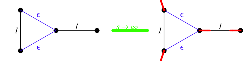
Figure 3: The system at the l. h. s. cannot be a DGS system for fixed $\epsilon>0$ and arbitrary $s$, since its classical limit at the r. h. s. is not DGS. The classical ground state is indicated by small arrows.

4.2

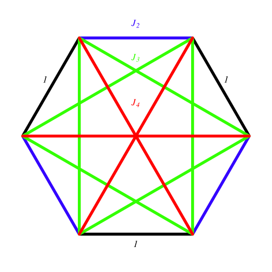
Figure 4: A system of $3$ dimers with special coupling constants $J_{1}=1,J_{2},J_{4}$ and $J_{3}=\frac{1}{2}(J_{2}+J_{4})$.

Another $s=1/2$ system for which ${\cal C}_{\Phi}$ can be directly calculated by the method sketched in section 3.3 consists of $3$ dimers with equal coupling strength $J_{1}$ and three further coupling constants $J_{2},J_{3},J_{4}$, see figure 4. According to theorem 1 we must have $J_{3}=\frac{1}{2}(J_{2}+J_{4})$ if this system has a DGS. Hence only three independent variables, say, $J_{1},J_{2}$ and $J_{4}$ are left. These define a $3$-dimensional subspace of ${\cal J}_{\Phi}$ and a corresponding sub-cone ${\cal C}^{\prime}_{\Phi}$ of ${\cal C}_{\Phi}$. ${\cal C}^{\prime}_{\Phi}$ can be represented by a convex subset ${\cal K}_{\Phi}$ of the $J_{2}-J_{4}-$plane which is the intersection of the cone ${\cal C}^{\prime}_{\Phi}$ and the hyperplane $J_{1}=1$. The permutation $(12)(34)(56)$ swaps $J_{2}$ and $J_{4}$ leaving ${\cal C}^{\prime}_{\Phi}$ invariant. Hence ${\cal K}_{\Phi}$ is symmetric w. r. t. reflections at the axis $J_{2}=J_{4}$.

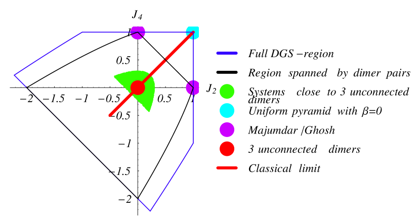
Figure 5: The set ${\cal K}_{\Phi}$ of points with coordinates $(J_{2},J_{4})$ such that the system shown in figure 4 is a DGS system. Certain prominent subsets and points are displayed which re explained in section 4.2.

${\cal K}_{\Phi}$ is bounded by the lines $J_{4}=1$, $J_{2}=1$ and $J_{4}+J_{2}=-2$ and by two curves with small but finite curvature which lie symmetric to the axis $J_{2}=J_{4}$, see figure 5. Prominent points of ${\cal K}_{\Phi}$ are

• $(1,1)\;:$ Uniform pyramid with $\beta=0$,

• $(1.0)$ and $(0,1)\;:$ Majumdar/Ghosh rings,

• $(0,0)\;:$ Three unconnected dimers.

The small neighborhood of $(0,0)$ which belongs to ${\cal K}_{\Phi}$ according to proposition 3 is also shown. We see that the bound in (19) is far from being optimal in this case. Further we have displayed the convex subset ${\cal L}_{\Phi}\subset{\cal K}_{\Phi}$ generated by three dimer pairs according to proposition 4
For larger $s>\frac{1}{2}$ the figures ${\cal K}_{\Phi}^{s}$ would shrink towards their classical limit which turns out to be the line segment

$$-\frac{1}{2}\leq J_{2}=J_{4}\leq 1\;.$$ (36)

As mentioned before, the boundary of ${\cal K}_{\Phi}$ corresponds to a degeneracy of the ground state. It is easy to identify the “rival" ground states for the straight parts of the boundary: If $J_{2}=1$ the second Majumdar/Ghosh dimerized state becomes a rival ground state, analogously for $J_{4}=1$. If the system approaches the line $J_{2}+J_{4}=-2$ the ferromagnetic ground state $|\uparrow\uparrow\uparrow\uparrow\uparrow\uparrow\rangle$ becomes the rival ground state. The curved parts of the boundary of ${\cal K}_{\Phi}$ correspond to continuously varying families of rival ground states.

5 Proofs

5.1 Proof of theorem 1

We rewrite the Hamiltonian (3) in the form

$$H({\mathbb{J}}) = \sum_{\mu\neq\nu}J_{\mu\nu}\>\bi{s}_{\mu}\cdot\bi{s}_{\mu}$$ (37)

$$= \sum_{i\neq j}\sum_{\epsilon,\delta=0}^{1}J_{i\epsilon,j\delta}\>\bi{s}_{i\epsilon}\cdot\bi{s}_{j\delta}+2\sum_{i=1}^{N}J_{i0,i1}\bi{s}_{i0}\cdot\bi{s}_{i1}$$ (38)

$$\equiv \sum_{i<j}\overline{H}_{ij}\;,$$ (39)

where the distribution of the terms of the second sum in (38) to the terms $\overline{H}_{ij}$ is arbitrary. We have $\overline{H}_{ij}=H_{ij}\otimes\;\smash{\raisebox{-2.15277pt}{$\!\!\stackrel{{\scriptstyle\!\mbox{1}\rule[0.0pt]{0.18082pt}{4.82224pt}}}{{}}$}}^{(ij)}$ such that $H_{ij}$ acts on ${\cal H}_{ij}={\cal H}_{i}\otimes{\cal H}_{j}$ and $\;\smash{\raisebox{-2.15277pt}{$\!\!\stackrel{{\scriptstyle\!\mbox{1}\rule[0.0pt]{0.18082pt}{4.82224pt}}}{{}}$}}^{(ij)}$ on the remaining factors. Recall that the dimerized state has the form

$$\Phi=\bigotimes_{i=1}^{N}[i0,i1]\;,$$ (40)

where $[i0,i1]$ denotes the AF dimer ground state (5) in ${\cal H}_{i}={\cal H}_{i0}\otimes{\cal H}_{i1}$.

Lemma 2

$\Phi$ is an eigenstate of $H({\mathbb{J}})$ iff $[i0,i1]\otimes[j0,j1]$ is an eigenstate of $H_{ij}$ for all $i<j=2,\ldots N$.

Proof: The if-part is obvious. To prove the only-if-part we consider an orthonormal basis $(e_{\lambda}^{(i)})_{\lambda=0,\ldots,L}$ in ${\cal H}_{i}$ such that $e_{0}^{(i)}=[i0,i1]$ where $L=(2s+1)^{2}-1$. The action of $H_{ij}$ on $[i0,i1]\otimes[j0,j1]$ may be written as

$$H_{ij}(e_{0}^{(i)}\otimes e_{0}^{(j)})=\sum_{\lambda,\mu=0}^{L}h_{\lambda\mu}^{(ij)}e_{\lambda}^{(i)}\otimes e_{\mu}^{(j)}\;.$$ (41)

Let $(e_{\lambda}^{(i)}\otimes e_{\mu}^{(j)})_{\Phi}\equiv e_{0}^{(1)}\otimes e_{0}^{(2)}\otimes\ldots e_{\lambda}^{(i)}\otimes\ldots e_{\mu}^{(j)}\otimes\ldots\otimes e_{0}^{(N)}$. Then

$$H({\mathbb{J}})\Phi = \sum_{i<j}\overline{H}_{ij}(e_{0}^{(i)}\otimes e_{0}^{(j)})_{\Phi}$$ (42)

$$= \sum_{i<j}\sum_{\lambda\mu}h_{\lambda\mu}^{(ij)}(e_{\lambda}^{(i)}\otimes e_{\mu}^{(j)})_{\Phi}=E\Phi=E\sum_{i<j}(e_{0}^{(i)}\otimes e_{0}^{(j)})_{\Phi}\;.$$ (43)

The terms at the l. h. s. of (43) proportional to $(e_{\lambda}^{(i)}\otimes e_{\mu}^{(j)})_{\Phi}$ with $\lambda,\mu=1,\ldots,L$ cannot cancel since they occur only once in the sum $\sum_{i<j}$. But they don’t occur at the r. h. s. of (43), hence $h_{\lambda\mu}^{(ij)}=0$ for all $\lambda,\mu=1,\ldots,L$. $H_{ij}$ maps the subspace of ${\cal H}_{ij}$ with total spin quantum number $S_{ij}=0$ onto itself, hence $h_{0\mu}^{(ij)}=h_{\lambda 0}^{(ij)}=0$ for all $\mu,\lambda=1,\ldots,L$. Thus only $h_{00}^{(ij)}$ may be non-zero, which means that $e_{0}^{(i)}\otimes e_{0}^{(j)}$ is an eigenstate of $H_{ij}$.  

In view of lemma 2 we only need to consider the case of $N=2$ dimers with indices $i<j$ in the remaining part of the proof. We set $\Phi=[i0,i1]\otimes[j0,j1]$ and rewrite the indices according to

$$(i0)\equiv 0,\>(i1)\equiv 1,\>(j0)\equiv 2,\>(j1)\equiv 3\;,$$ (44)

Consider a modified Hamiltonian of the form

$$H^{\prime}=\sum_{(\mu\nu)\in\{02,03,12,13\}}J_{\mu\nu}\bi{s}_{\mu}\cdot\bi{s}_{\nu}\;.$$ (45)

Obviously, $\Phi$ is an eigenvector of $H_{ij}$ iff it is an eigenvector of $H^{\prime}$, since the difference between $H_{ij}$ and $H^{\prime}$ consists of two dimer Hamiltonians. We note that for fixed $\mu\in\{0,1,2,3\}$ the three operators $\bi{s}_{\mu}^{(i)},i=1,2,3$ form an “irreducible tensor operator", i. e. they span a $3$-dimensional irreducible subspace with quantum number $S=1$. Here and henceforward “irreducible" will always be understood as “irreducible w. r. t. the product representation of $SU(2)$ in ${\cal H}_{ij}$ (or similar spaces)". In order to apply the Wigner-Eckhardt theorem (WE), see for example [22], we consider states of the form

$$\psi=\psi_{01}\otimes\psi_{23}\;,$$ (46)

such that $\psi_{01}\in{\cal H}_{01}$ (resp. $\psi_{23}\in{\cal H}_{23}$) belong to irreducible subspaces of ${\cal H}_{01}$ (resp. ${\cal H}_{23}$) characterized by their dimension $2S_{01}+1$ (resp. $2S_{23}+1$). Recall that WE yields “selection rules" of the following kind: The matrix element of a component of a tensor operator with representation $D$ between two states belonging to irreducible representations $D_{1}$ and $D_{2}$ is nonzero only if $D$ is contained in the product representation of $D_{1}$ and $D_{2}$. In the case of irreducible $SU(2)$ representations which are characterized by quantum numbers, say, $S$, $S_{1}$ and $S_{2}$, the above condition simply reads: $|S_{1}-S_{2}|\leq S\leq S_{1}+S_{2}$. The dimer ground states $[01]$ and $[23]$ of course span $S_{2}=0$ representations. Then WE yields:

Lemma 3

$\langle\psi|H^{\prime}|\Phi\rangle\neq 0$ only if $S_{01}=S_{23}=1$.

Proof: It will suffice to consider only one term of $H^{\prime}$, for example $J_{02}\bi{s}_{0}^{(i)}\otimes\bi{s}_{2}^{(i)}$, since analogous arguments apply for the other terms. We skip the factor $J_{02}$ and write

$$\langle\psi|\bi{s}_{0}^{(i)}\otimes\bi{s}_{2}^{(i)}|\Phi\rangle = \langle\psi_{01}\otimes\psi_{23}|\bi{s}_{0}^{(i)}\otimes\bi{s}_{2}^{(i)}|[01]\otimes[23]\rangle$$ (47)

$$= \langle\psi_{01}|\bi{s}_{0}^{(i)}|[01]\rangle\langle\psi_{23}|\bi{s}_{2}^{(i)}|[23]\rangle\;.$$ (48)

The first factor vanishes by WE if $S_{01}\neq 1$, the second one if $S_{23}\neq 1$.  
Especially, $\langle\Phi|H^{\prime}|\Phi\rangle=0$ and hence, if $\Phi$ is an eigenvector of $H^{\prime}$ the corresponding eigenvalue can only be zero.
It is well-known that the irreducible subspaces of ${\cal H}_{01}$ are eigenspaces of the permutation $\pi_{01}$ with eigenvalues $(-1)^{S_{01}+2s}$, analogously for $\pi_{23}$. For example, if $s=1/2$, the $S_{01}=0$ singlet subspace of ${\cal H}_{01}$ is spanned by the antisymmetric state $\frac{1}{\sqrt{2}}(\uparrow\downarrow-\downarrow\uparrow)$, whereas the $S_{01}=1$ triplet subspace is symmetric. The terms $\bi{s}_{\mu}\cdot\bi{s}_{\nu}$ occurring in $H^{\prime}$ can be generated from $\bi{s}_{0}\cdot\bi{s}_{2}$ by applying suitable permutations $\pi_{01}$ and $\pi_{23}$. Hence, using lemma 3 and the above-mentioned symmetry of $\psi$ under permutations, we obtain

$$\langle\psi|H^{\prime}|\Phi\rangle = \sum_{(\mu\nu)\in\{02,03,12,13\}}J_{\mu\nu}\langle\psi|\bi{s}_{\mu}\cdot\bi{s}_{\nu}|\Phi\rangle$$ (49)

$$= (J_{02}+J_{13}-J_{03}-J_{12})\langle\psi|\bi{s}_{0}\cdot\bi{s}_{2}|\Phi\rangle\;.$$ (50)

Since $\langle\psi|\bi{s}_{0}\cdot\bi{s}_{2}|\Phi\rangle\neq 0$ for a suitable $\psi$ we conclude that $J_{02}+J_{13}-J_{03}-J_{12}=0$ iff $H^{\prime}\Phi=0$ iff $\Phi$ is an eigenvector of $H^{\prime}$. Together with lemma 2 this concludes the proof of theorem 1.

5.2 Proof of proposition 1

Using the same notation as in section 5.1 we conclude by WE that

$$\langle[01]\otimes\psi_{23}\left|\bi{s}_{\mu}^{(i)}\otimes\bi{s}_{\nu}^{(i)}\right|[01]\otimes\psi_{23}\rangle = \langle[01]\left|\bi{s}_{\mu}^{(i)}\right|[01]\rangle\langle\psi_{23}\left|\bi{s}_{\nu}^{(i)}\right|\psi_{23}\rangle=0$$ (51)

for all $(\mu\nu)\in\{02,03,12,13\}$. For fixed $j\in\{1,\ldots,N\}$ let

$$\Phi^{\prime}=\bigotimes_{\stackrel{{\scriptstyle\scriptstyle i=1}}{{(i\neq j)}}}^{N}[i0,i1]\otimes|s,s\rangle\;,$$ (52)

where $|s,s\rangle$ is the ferromagnetic ground state in ${\cal H}_{j}$. By (51) and analogous equations for permuted indices the expectation value $\langle\Phi^{\prime}\left|H({\mathbb{J}})\right|\Phi^{\prime}\rangle$ contains no interaction terms between dimers and thus

$$\langle\Phi^{\prime}\left|H({\mathbb{J}})\right|\Phi^{\prime}\rangle = 2\left[-\sum_{\stackrel{{\scriptstyle\scriptstyle i=1}}{{(i\neq j)}}}^{N}J_{i0,i1}s(s+1)+J_{j0,j1}s^{2}\right]$$ (54)

$$\geq\langle\Phi\left|H({\mathbb{J}})\right|\Phi\rangle=2\left[-\sum_{i=1}^{N}J_{i0,i1}s(s+1)\right]\;.$$

In (54) we used the assumption of proposition 1 that $\Phi$ is a ground state of $H({\mathbb{J}})$. It follows that $J_{j0,j1}s^{2}\geq-J_{j0,j1}s(s+1)$ and hence $J_{j0,j1}\geq 0$, which concludes the proof.

5.3 Proof of theorem 2

First we want to show that (10) also holds for classical DGS systems.

Lemma 4

Let ${\mathbb{J}}\in{\cal C}_{\Phi}^{\small{cl}}$. Then

$$\widetilde{J}_{ij}\equiv J_{i0,j0}+J_{i1,j1}-J_{i0,j0}-J_{i1,j0}=0$$ (55)

for all $i<j=2,\ldots,N$.

Proof: By assumption, any classical state $\bi{s}$ satisfying

$$\bi{s}_{i0}+\bi{s}_{i1}=\bi{0}\mbox{ for all }i=1,\ldots,N$$ (56)

minimizes the energy $H({\mathbb{J}},\bi{s})$. For such states we may write

$$H({\mathbb{J}},\bi{s}) = \sum_{\mu\neq\nu}J_{\mu\nu}\bi{s}_{\mu}\cdot\bi{s}_{\nu}$$ (57)

$$= 2\sum_{1\leq i<j\leq N}\sum_{\epsilon,\delta=0}^{1}J_{i\epsilon,j\delta}\;\bi{s}_{i\epsilon}\cdot\bi{s}_{j\delta}-2\sum_{i=1}^{N}J_{i0,i1}$$ (59)

$$= 2\sum_{1\leq i<j\leq N}\left(J_{i0,j0}+J_{i1,j1}-J_{i0,j1}-J_{i1,j0}\right)\bi{s}_{i0}\cdot\bi{s}_{j0}$$

$$-2\sum_{i=1}^{N}J_{i0,i1}\;.$$

The function $\bi{s}\mapsto H({\mathbb{J}},\bi{s})$ is constant for all $\bi{s}\in{\cal P}$ satisfying (56). The above equations show that also the function $(\bi{s}_{i})_{i=1,\ldots,N}\mapsto\widetilde{H}(\bi{s})\equiv\sum_{1\leq i<j\leq N}\widetilde{J}_{ij}\bi{s}_{i}\cdot\bi{s}_{j}$ is constant. We write

$$\widetilde{H}(\bi{s})=\bi{s}_{1}\cdot\sum_{2\leq j\leq N}\widetilde{J}_{1j}\bi{s}_{j}+\sum_{2\leq i<j\leq N}\widetilde{J}_{ij}\bi{s}_{i}\cdot\bi{s}_{j}\;.$$ (60)

Since $\widetilde{H}(\bi{s})$ is independent of $\bi{s}_{1}$, the second factor in the first scalar product in (60) must vanish: $\sum_{2\leq j\leq N}\widetilde{J}_{1j}\bi{s}_{j}=0$. By choosing $\bi{s}_{j}\perp\bi{s}_{2}$ for all $j>2$ we conclude $\widetilde{J}_{12}=0$. This concludes the proof of the proposition since the numbering of the dimers is arbitrary.  
Next we want to show (12):

Lemma 5

If ${\mathbb{J}}\in{\cal C}_{\Phi}^{\small{cl}}$ then

$$J_{i0,j0}=J_{i0,j1}=J_{i1,j0}=J_{i1,j1}\equiv\epsilon_{ij}$$ (61)

Proof: It will suffice to show $J_{i0,j1}=J_{i1,j0}$, since $J_{i0,j0}=J_{i1,j1}$ follows by applying the permutation $(01)$ and the remaining identity $J_{i0,j1}=J_{i0,j0}$ by (55).
Consider the state $\bi{s}(\alpha)$ defined by

$$\bi{s}_{i0} = {\left(\begin{array}[]{r}1\\ 0\\ 0\end{array}\right)},\bi{s}_{i1}={\left(\begin{array}[]{r}-\cos\alpha\\ \sin\alpha\\ 0\end{array}\right)},\bi{s}_{j0}={\left(\begin{array}[]{r}0\\ 1\\ 0\end{array}\right)},\;\bi{s}_{j1}={\left(\begin{array}[]{r}-\sin\alpha\\ -\cos\alpha\\ 0\end{array}\right)}$$ (74)

and

$$\bi{s}_{k0} = -\bi{s}_{k1}={\left(\begin{array}[]{r}0\\ 0\\ 1\end{array}\right)}\mbox{ for all }k\neq i,j.$$ (78)

Here $\alpha$ is an arbitrary angle $0\leq\alpha<\pi$ to be fixed later. Let $E(\alpha)$ denote the energy of this state. We conclude

$$\frac{1}{2}E(\alpha) = J_{i0,i1}\bi{s}_{i0}\cdot\bi{s}_{i1}+J_{j0,j1}\bi{s}_{j0}\cdot\bi{s}_{j1}+J_{i0,j0}\bi{s}_{i0}\cdot\bi{s}_{j0}+J_{i1,j1}\bi{s}_{i1}\cdot\bi{s}_{j1}$$ (79)

$$+J_{i0,j1}\bi{s}_{i0}\cdot\bi{s}_{j1}+J_{i1,j0}\bi{s}_{i1}\cdot\bi{s}_{j0}-\sum_{\stackrel{{\scriptstyle\scriptstyle k=1}}{{(k\neq i,j)}}}J_{k0,k1}$$

$$= -\left(J_{i0,i1}+J_{j0,j1}\right)\cos\alpha+\left(J_{i1,j0}-J_{i0,j1}\right)\sin\alpha-\sum_{\stackrel{{\scriptstyle\scriptstyle k=1}}{{(k\neq i,j)}}}J_{k0,k1}$$ (80)

$$= \left(J_{i0,i1}+J_{j0,j1}\right)(1-\cos\alpha)+\left(J_{i1,j0}-J_{i0,j1}\right)\sin\alpha+\frac{1}{2}E(0)\;.$$ (81)

It is obvious that the state $\bi{s}(\alpha)$ defined by (74) and (78) is a classical DGS for $\alpha=0$, hence $E(0)$ is the ground state energy. If $J_{i0,i1}+J_{j0,j1}\leq 0$ and $J_{i1,j0}-J_{i0,j1}\neq 0$ we may choose the sign of $\alpha$ such that $E(\alpha)<E(0)$ which is impossible due to the last statement. Thus we may assume $J_{i0,i1}+J_{j0,j1}>0$. Hence the expression (81) has its minimum at a value $\alpha=\alpha_{0}$ defined by

$$\tan\alpha_{0}=-\frac{J_{i1,j0}-J_{i0,j1}}{J_{i0,i1}+J_{j0,j1}}\;.$$ (82)

After some algebra we obtain for the corresponding energy

$$\frac{1}{2}E(\alpha_{0})=(J_{i0,i1}+J_{j0,j1})\left(1-\sqrt{1+\left(\frac{J_{i1,j0}-J_{i0,j1}}{J_{i0,i1}+J_{j0,j1}}\right)^{2}}\right)+\frac{1}{2}E(0)\;,$$ (83)

which is less than $\frac{1}{2}E(0)$ if not $J_{i1,j0}-J_{i0,j1}=0$.  
It remains to show (13):

Lemma 6

If ${\mathbb{J}}\in{\cal C}_{\Phi}^{\small{cl}}$ then

$$J_{i0,i1}\geq 0$$ (84)

for all $i=1,\ldots,N$.

Proof: We rewrite $H({\mathbb{J}},\bi{s})$ using (61), $\mu_{i}\equiv J_{i0,i1}$ and $\bi{S}_{i}\equiv\bi{s}_{i0}+\bi{s}_{i1}$, $\bi{S}_{ij}\equiv\bi{S}_{i}+\bi{S}_{j}$ for $i<j=2,\ldots,N$:

$$H({\mathbb{J}},\bi{s}) = 2\sum_{i=1}^{N}\mu_{i}\bi{s}_{i0}\cdot\bi{s}_{i1}$$ (85)

$$+ 2\sum_{1\leq i<j\leq N}\epsilon_{ij}(\bi{s}_{i0}\cdot\bi{s}_{j0}+\bi{s}_{i1}\cdot\bi{s}_{j0}+\bi{s}_{i0}\cdot\bi{s}_{j1}+\bi{s}_{i1}\cdot\bi{s}_{j1})$$

$$= \sum_{i=1}^{N}\mu_{i}(\bi{S}_{i}^{2}-2)+\sum_{1\leq i\neq j\leq N}\epsilon_{ij}\bi{S}_{i}\cdot\bi{S}_{j}\;.$$ (86)

The energy of the DGS will be $E_{0}=-2\sum_{i=1}^{N}\mu_{i}$. Assume that for some $i\in\{1,\ldots,N\}$ we have $\mu_{i}<0$ and consider a state $\bi{s}$ such that $\bi{S}_{j}=\bi{0}$ for all $j\neq i$ and $|\bi{S}_{i}|=2$. For this state we obtain $H({\mathbb{J}},\bi{s})=4\mu_{i}+E_{0}$ which contradicts the assumption that the system has a DGS.  
This completes the proof of theorem 2.

5.4 Proof of theorem 3

In order to prove theorem 3 we stick to the notation of the last section and rewrite the energy of a classical DGS system (86) in the form

$$E(\vec{S})=\langle\vec{S}|{\mathbb{M}}|\vec{S}\rangle-2\sum_{i=1}^{N}\mu_{i}\;.$$ (87)

Here $\vec{S}$ denotes a $3N$-dimensional vector with components

$$\vec{S}=(S_{1}^{(1)},S_{1}^{(2)},S_{1}^{(3)},\ldots,S_{N}^{(1)},S_{N}^{(2)},S_{N}^{(3)})\;,$$ (88)

and ${\mathbb{M}}\equiv{\mathbb{G}}\otimes\;\smash{\raisebox{-2.15277pt}{$\!\!\stackrel{{\scriptstyle\!\mbox{1}\rule[0.0pt]{0.18082pt}{4.82224pt}}}{{}}$}}_{\>{}_{3}}$, where $\;\smash{\raisebox{-2.15277pt}{$\!\!\stackrel{{\scriptstyle\!\mbox{1}\rule[0.0pt]{0.18082pt}{4.82224pt}}}{{}}$}}_{\>3}$ is the $3\times 3$ unit matrix and ${\mathbb{G}}$ has the components

$$G_{ii} = \mu_{i},\;i=1,\ldots,N$$ (89)

$$G_{ij} = \epsilon_{ij},\;1\leq i\neq j\leq N\;.$$ (90)

We have to show that the system is DGS iff ${\mathbb{M}}$, or, equivalently, ${\mathbb{G}}$ is positive semi-definite. This follows immediately from ${\mathbb{M}}\geq 0$ iff $E(\vec{S})\geq-2\sum_{i=1}^{N}\mu_{i}=E_{0}$ for all $\vec{S}$ such that $|\bi{S}_{i}|\leq 2$ for all $i=1,\ldots,N$.

5.5 Proof of proposition 2

Due to (3.1) and (15) the Hamiltonian of a uniform pyramid can be written as

$$H({\mathbb{J}})=(\alpha-\beta)(\bi{S}_{N}^{2}-2Ns(s+1))+\beta\left[(\bi{S}_{N}+\bi{s}_{N+1,0})^{2}-(2N+1)s(s+1)\right],$$ (91)

where

$$\bi{S}_{N}\equiv\sum_{i=1}^{N}\sum_{\delta=0}^{1}\bi{s}_{i\delta}\;.$$ (92)

The eigenvalues of $\bi{S}_{N}^{2}$ are of the form $S(S+1)$, where $S=0,1,\ldots,2Ns$. Obviously, the choice $S=0$ minimizes (91) if $\beta$ is small enough. In this case $\Phi$ is a ground state since it has $S=0$. If $\beta$ increases, it will eventually reach a certain value $\beta_{0}$ where $S=1$ states have the same energy as $\Phi$. The other values $S>1$ can be excluded. For $\beta=\beta_{0}$ and $s>1/2$ the coincidence of the energies implies

$$(\alpha-\beta_{0})(-2Ns(s+1)) + \beta_{0}(s(s+1)-(2N+1)s(s+1))$$

$$=(\alpha-\beta_{0})(1\cdot 2-2Ns(s+1)) + \beta_{0}((s-1)s)-(2N+1)s(s+1)\;,$$ (93)

hence

$$\beta_{0}=\frac{\alpha}{1+s}$$ (94)

and the system has a DGS for $\beta\leq\beta_{0}$. The value $\beta_{0}=\alpha$ in the case $s=1/2$ follows analogously. The only difference is that in this case the minimal eigenvalue of $(\bi{S}_{N}+\bi{s}_{N+1,0})^{2}$ will be $s(s+1)=3/4$ and not $(s-1)s$ as in the case $s>1/2$.

5.6 Proof of proposition 3

We consider the matrix $\stackrel{{\scriptstyle\circ}}{{\mathbb{J}}}$ of a system of $N$ uncoupled AF dimers, i. e.

$$\lambda_{i}\equiv\stackrel{{\scriptstyle\circ}}{{J}}_{i0,i1}>0\mbox{ for all }i=1,\ldots,N\mbox{ and }\stackrel{{\scriptstyle\circ}}{{J}}_{\mu\nu}=0\mbox{ else.}$$ (95)

Without loss of generality we may assume

$$\lambda_{1}=\lambda\equiv\min\{\lambda_{i}|i=1\ldots N\}\;.$$ (96)

The other assumptions are as in proposition 3. Let $\delta_{\small{min}}$ denote the lowest eigenvalue of $\Delta$, hence ${\cal x}(\Delta)=|\delta_{\small{min}}|$. Consider any $\Psi\in{\cal H}$ such that $\|\Psi\|=1$ and $\Psi\perp\Phi$. The two lowest eigenvalues of $H(\stackrel{{\scriptstyle\circ}}{{\mathbb{J}}})$ are

$$E_{0} = -2s(s+1)\sum_{i=1}^{N}\lambda_{i}\quad\mbox{and}$$ (97)

$$E_{1} = -2s(s+1)\sum_{i=2}^{N}\lambda_{i}+\lambda_{1}(2-2s(s+1))$$ (98)

$$= E_{0}+2\lambda_{1}\;.$$ (99)

$E_{0}$ belongs to the non-degenerate eigenvector $\Phi$, hence

$$E_{1}\leq\langle\Psi|H(\stackrel{{\scriptstyle\circ}}{{\mathbb{J}}})|\Psi\rangle\;.$$ (100)

The expectation value of the Hamiltonian $H(\Delta)$ can be estimated as follows

$$\langle\Psi|H(\Delta)|\Psi\rangle = \sum_{\mu\nu}\Delta_{\mu\nu}\langle\Psi|\bi{s}_{\mu}\cdot\bi{s}_{\nu}|\Psi\rangle$$ (101)

$$\geq \delta_{\small{min}}\sum_{\mu}\langle\Psi|\bi{s}_{\mu}^{2}|\Psi\rangle=\delta_{\small{min}}Ns(s+1)$$ (102)

$$\geq -2\lambda_{1}\;,$$ (103)

using (19) and $\delta_{\small{min}}<0$ since $\Tr(\Delta)=0$. Thus

$$\langle\Psi|H({\mathbb{J}})|\Psi\rangle = \langle\Psi|H(\stackrel{{\scriptstyle\circ}}{{\mathbb{J}}})|\Psi\rangle+\langle\Psi|H(\Delta)|\Psi\rangle$$ (104)

$$\geq E_{1}-2\lambda_{1}=E_{0}\;,$$ (105)

using (100), (103) and (99). This proves that $\Phi$ is a ground state of $H({\mathbb{J}})$.

5.7 Proof of proposition 5

Let ${\mathbb{J}}\in{\cal C}_{\Phi}^{\small{cl}}$ and $\Psi\in{\cal H},\;\|\Psi\|=1$. Then

$$\langle\Psi|H({\mathbb{J}})|\Psi\rangle = \sum_{i=1}^{N}G_{ii}(\langle\Psi|\bi{S}_{i}^{2}|\Psi\rangle-2)+\sum_{1\leq i\neq j\leq N}G_{ij}(\langle\Psi|\bi{S}_{i}\cdot\bi{S}_{j}|\Psi\rangle$$ (106)

$$= \Tr{\mathbb{G}}{\mathbb{W}}+E_{0}\;,$$ (107)

where ${\mathbb{W}}$ is an $N\times N$- matrix with elements

$$W_{ij}=\langle\Psi|\bi{S}_{i}\cdot\bi{S}_{j}|\Psi\rangle\mbox{ and }E_{0}=\langle\Phi|H({\mathbb{J}})|\Phi\rangle\;.$$ (108)

It can be easily shown that ${\mathbb{W}}\geq 0$. Since also ${\mathbb{G}}\geq 0$ by theorem 3 we may conclude that $\Tr({\mathbb{G}}{\mathbb{W}})\geq 0,\;\langle\Psi|H({\mathbb{J}})|\Psi\rangle\geq E_{0}$ and hence ${\mathbb{J}}\in{\cal C}_{\Phi}^{s}$ for all $s=1/2,1,3/2,\ldots$.

6 Geometrical structure of ${\cal C}_{\Phi}$

The defining inequalities of ${\mathbb{J}}\in{\cal C}_{\Phi}$ are

$$\langle\Phi|H({\mathbb{J}})|\Phi\rangle\leq\langle\psi|H({\mathbb{J}})|\psi\rangle\mbox{ for all }\psi\in{\cal H},\;\|\psi\|=1\;.$$ (109)

For fixed $\psi,\;\psi\neq\Phi,$ (109) defines a closed half space of the real linear space ${\cal J}_{\Phi}$. Thus ${\cal C}_{\Phi}$ is an intersection of closed half spaces and hence a closed convex cone. For the notion of a cone and related notions, see, for example, [23].
Moreover, ${\cal C}_{\Phi}$ is a proper cone, i. e. ${\mathbb{J}},-{\mathbb{J}}\in{\cal C}_{\Phi}$ implies ${\mathbb{J}}=0$. Indeed, ${\mathbb{J}},-{\mathbb{J}}\in{\cal C}_{\Phi}$ means that $\langle\Phi|H({\mathbb{J}})|\Phi\rangle$ is simultaneously the lowest and the highest eigenvalue of $H({\mathbb{J}})$, which, due to $\Tr H({\mathbb{J}})=0$, implies $H({\mathbb{J}})=0$ and ${\mathbb{J}}=0$.
The set of differences ${\cal C}_{\Phi}-{\cal C}_{\Phi}$ is a linear subspace of ${\cal J}_{\Phi}$; by virtue of proposition 3 ${\cal C}_{\Phi}$ contains interior points and hence ${\cal C}_{\Phi}-{\cal C}_{\Phi}={\cal J}_{\Phi}$. In other words, ${\cal J}_{\Phi}$ is a generating cone.

A face $F$ is a convex subset of a convex set ${\cal C}$ such that $\lambda c_{1}+(1-\lambda)c_{2}\in F,\;c_{1},c_{2}\in{\cal C},\;0<\lambda<1$ implies $c_{1}\in F$ and $c_{2}\in F$. In words: If a point of $F$ lies in the interior of a segment contained in ${\cal C}$, then the endpoints of that segment will also lie in $F$. A proper face is a face different from $\emptyset$ and ${\cal C}$. Special faces are the singletons $F=\{f\}$, such that $f$ never lies in the interior of a segment contained in ${\cal C}$; such $f$ are called extremal points of ${\cal C}$. The dimension $d$ of a face $F$ is defined as the dimension of the affine subspace generated by $F$. Hence extremal points can be viewed as $0$-dimensional faces. The above definitions follow, for example, [24]; other authors reserve the notion of a “face" to the intersection of ${\cal C}$ with a supporting hyperplane. By virtue of theorem 4 both notions coincide for the faces of ${\cal C}_{\Phi}$. The boundary of a closed convex set ${\cal C}$ in a finite-dimensional linear space is the union of its faces $F$, excluding $F={\cal C}$. The set of all faces of ${\cal C}$ will form a lattice w. r. t. the set-theoretic inclusion of faces, such that $F_{1}\wedge F_{2}=F_{1}\cap F_{2}$, but $F_{1}\vee F_{2}$ will be the smallest face containing $F_{1}$ and $F_{2}$, which in general larger than $F_{1}\cup F_{2}$.

It is possible to more closely characterize the faces of ${\cal C}_{\Phi}$. To this end we note that the definition (109) of ${\cal C}_{\Phi}$ does not make use of the special form of $\Phi$ as a product of dimer ground states. Hence ${\cal C}_{\phi}$ may defined for arbitrary normalized states $\phi\in{\cal H}$. We will, however, always restrict this definition to ${\mathbb{J}}\in{\cal J}_{\Phi}$ such that ${\cal C}_{\phi}$ will be a closed proper convex cone in ${\cal J}_{\Phi}$ also for the general case.

Theorem 4

All faces $F$ of ${\cal C}_{\Phi}$ are of the form

$$F=\bigcap_{i=0}^{k}{\cal C}_{\phi_{i}}\;,$$ (110)

where $\phi_{0}=\Phi,\;\phi_{i}\in{\cal H},$ and $\langle\phi_{i},\phi_{j}\rangle=\delta_{ij}$ for all $i,j=0,\ldots,k$.
Conversely, any intersection of the form (110) will be a, possibly empty, face of ${\cal C}_{\Phi}$.

The special case $F={\cal C}_{\Phi}$ is included in (110) with $k=0$. If ${\mathbb{J}}$ lies at the boundary of ${\cal C}_{\Phi}$, it is contained in a proper face of ${\cal C}_{\Phi}$ and hence there will be at least one further ground state different from $\Phi$. Hence we have the following:

Corollary 2

${\mathbb{J}}$ is an interior point of ${\cal C}_{\Phi}$ iff $\Phi$ is a non-degenerate ground state of $H({\mathbb{J}})$.

Proof of theorem 4:

1. Let $F=\bigcap_{i=0}^{k}{\cal C}_{\phi_{i}}$ be given with the properties stated in the theorem. We want to show that $F$ is a face. Clearly, $F$ is a convex subset of ${\cal C}_{\Phi}$. Assume ${\mathbb{J}}=\lambda{\mathbb{J}}_{1}+(1-\lambda){\mathbb{J}}_{2}\in F,\;{\mathbb{J}}_{i}\in{\cal C}_{\Phi},\;0<\lambda<1$. If $k=0$ we are done, hence we may assume $k>0$. Let $E_{i}\equiv\langle\Phi|H({\mathbb{J}}_{i})|\Phi\rangle$ denote the ground state energies and $E^{\prime}_{i}\equiv\langle\phi_{1}|H({\mathbb{J}}_{i})|\phi_{1}\rangle$. By assumption,

   $$\lambda E^{\prime}_{1}+(1-\lambda)E^{\prime}_{2}=\langle\phi_{1}|H({\mathbb{J}})|\phi_{1}\rangle = \langle\Phi|H({\mathbb{J}})|\Phi\rangle$$ (111)

   $$= \lambda E_{1}+(1-\lambda)E_{2},$$ (112)

   hence

   $$\lambda(E^{\prime}_{1}-E_{1})+(1-\lambda)(E^{\prime}_{2}-E_{2}) = 0\;.$$ (113)

   In (113) both terms are non-negative since $E_{1}$ and $E_{2}$ are ground state energies. Hence $E^{\prime}_{1}=E_{1}$ and $\phi_{1}$ is a ground state of $H({\mathbb{J}}_{1})$. The same holds for all $\phi_{i},\;i=2,\ldots,k$. This means that ${\mathbb{J}}_{1}\in F$, analogously ${\mathbb{J}}_{2}\in F$, and thus $F$ is a face of ${\cal C}_{\Phi}$. During this proof we will call faces of this kind standard faces.

2. We will prove the following:

   Lemma 7

   Each boundary point of a standard face of ${\cal C}_{\Phi}$ is contained in a smaller standard face.

   Proof: Let $F$ be a standard face of the form (110) and $L$ a line in ${\cal J}_{\Phi}$ such that

   $$F\cap L=\{\lambda{\mathbb{J}}_{1}+(1-\lambda){\mathbb{J}}_{2}|0\leq\lambda\leq 1\},\;{\mathbb{J}}_{1}\neq{\mathbb{J}}_{2}\;.$$ (114)

   Obviously, ${\mathbb{J}}_{1}$ and ${\mathbb{J}}_{2}$ are boundary points, and every boundary point of $F$ can be obtained in this way. We consider the $1$-parameter analytic family of Hamiltonians $H(\lambda)=H(\lambda{\mathbb{J}}_{1}+(1-\lambda){\mathbb{J}}_{2})$. There exists a complete set of eigenvectors $\psi_{j}(\lambda)$ of $H(\lambda)$ such that the corresponding eigenvalues $E_{j}(\lambda)$ are analytical functions in some neighborhood of $\lambda=0$, see, for example, [25] theorem 7.10.1. We may arrange the indices such that the first $k+1$ eigenfunctions $\psi_{0}(\lambda),\ldots,\psi_{k}(\lambda)$ are degenerate and span the same eigenspace of $H(\lambda)$ as the $\phi_{i},\;i=0,\ldots,k$ for all $\lambda\in[0,1]$. According to the cited theorem they must also be degenerate for $\lambda\in(-\epsilon,0)$ for some small $\epsilon>0$ since an analytical function is constant on its total domain of definition if it is locally constant. But for $\lambda\in(-\epsilon,0)$ the ground states of $H(\lambda)$ must be other eigenvectors, say $\psi_{k+1}(\lambda),\ldots,\psi_{\ell}(\lambda)$, since $\lambda{\mathbb{J}}_{1}+(1-\lambda){\mathbb{J}}_{2}\notin F$. By continuity, $\psi_{k+1}(0),\ldots,\psi_{\ell}(0)$ are still ground states of $H(0)$. We thus conclude ${\mathbb{J}}_{2}\in\bigcap_{i=0}^{\ell}{\cal C}_{\phi_{i}}$ if $\phi_{k+1}\equiv\psi_{k+1}(0),\ldots,\phi_{\ell}\equiv\psi_{\ell}(0)$. This proves lemma 7.

3. It remains to show that each face $F$ of ${\cal C}_{\Phi}$ is a standard face. First consider the case where $F$ does not consist of a single extremal point. Let ${\mathbb{J}}\in F$ be an interior point of $F$ and $(\phi_{i})_{i=0,\ldots,k}$ an orthonormal basis of the eigenspace of $H({\mathbb{J}})$ corresponding to its lowest eigenvalue $E_{0}$. We may set $\phi_{0}=\Phi$. Let ${\mathbb{J}}_{1}\in F$ be arbitrary, but ${\mathbb{J}}_{1}\neq{\mathbb{J}}$ and consider $H(\lambda)=H(\lambda{\mathbb{J}}+(1-\lambda){\mathbb{J}}_{1}),\;\lambda\in{\mathbb{R}},\;$ as well as the affine functions $\lambda\mapsto\langle\phi_{i}|H(\lambda)|\phi_{i}\rangle,\;i=0,\ldots,k$. They coincide at $\lambda=1$ since $\langle\phi_{i}|H(1)|\phi_{i}\rangle=\langle\phi_{i}|H({\mathbb{J}})|\phi_{i}\rangle=E_{0}$. For some neighborhood of $\lambda=1$, $\lambda{\mathbb{J}}+(1-\lambda){\mathbb{J}}_{1}\in{\cal C}_{\Phi}$, since ${\mathbb{J}}$ is an interior point of $F$. Hence $\Phi$ is a ground state of of $H(\lambda)$ and $\langle\Phi|H(\lambda)|\Phi\rangle$ is the minimum of the functions $\lambda\mapsto\langle\phi_{i}|H(\lambda)|\phi_{i}\rangle,\;i=0,\ldots,k$. This is impossible unless these functions coincide for all $\lambda\in{\mathbb{R}}$. It follows that ${\mathbb{J}}_{1}\in\bigcap_{i=0}^{k}{\cal C}_{\phi_{i}}\equiv K$. Hence $F$ is contained in the standard face $K$. This holds also in the case of $F$ consisting of a single extremal point.
   If $F$ is not equal to $K$ it must be part of its boundary since $F$ is a face. If ${\mathbb{J}}$ is an interior point of $F$, as before, it must lie at the boundary of $K$ and, by lemma 7, must be contained in a smaller standard face $K^{\prime}=\bigcap_{i=0}^{\ell}{\cal C}_{\phi_{i}},\;\ell>k$. This is a contradiction since the ground states of $H({\mathbb{J}})$ are $\phi_{0},\ldots,\phi_{k}$, see above.
   Thus $F=K$, i. e. every face of ${\cal C}_{\Phi}$ is a standard face and the proof of theorem 4 is complete.

 
It will often be convenient to represent the cone ${\cal C}_{\Phi}$ by its intersection ${\cal K}_{\Phi}={\cal C}_{\Phi}\cap P$ with a suitable hyperplane $P$, see e. g. the example in section 4.2. It follows that the faces of ${\cal C}_{\Phi}$ are in $1:1$ correspondence with the faces of the closed convex set ${\cal K}_{\Phi}$, except for the vertex ${\mathbb{J}}=0$ of the cone ${\cal C}_{\Phi}$. The boundary of ${\cal K}_{\Phi}$ is partly flat, consisting of faces with dimension $d\geq 1$, partly curved, consisting of extremal points ${\mathbb{J}}$ of ${\cal K}_{\Phi}$ not contained in larger faces except ${\cal K}_{\Phi}$ itself. For these extremal points ${\mathbb{J}}$ the ground state of $H({\mathbb{J}})$ is two-fold degenerate: $\{{\mathbb{J}}\}=\bigcap_{i=0}^{1}{\cal C}_{\phi_{i}}$. It is already maximally degenerate in the sense that any smaller face $\bigcap_{i=0}^{2}{\cal C}_{\phi_{i}}$ will be empty.
Finally we note that throughout this section we never used the special structure of $\Phi$ as a product of AF dimer ground states. Hence our analysis will also apply to the cones ${\cal C}_{\phi}$ defined by other ground states $\phi$, but probably the dimerized ground state cone ${\cal C}_{\Phi}$ will show the richest structure compared with other cones ${\cal C}_{\phi}$.

7 Summary

In this article the classes ${\cal C}_{\Phi}^{s}$ of DGS systems have been investigated and completely characterized in the classical case $s=\infty$. In the quantum case we calculated the linear space ${\cal J}_{\Phi}$ generated by ${\cal C}_{\Phi}^{s}$, but ${\cal C}_{\Phi}^{s}$ itself could only be explicitely determined for small $N$ and $s$. In the general case, a “lower bound" ${\cal C}^{\prime}\subset{\cal C}_{\Phi}^{s}$ was constructed as the convex hull of three (resp. four) special subsets of ${\cal C}_{\Phi}^{s}$ for arbitrary $s$ (resp. $s=1/2$). The facial structure of the convex cone ${\cal C}_{\Phi}^{s}$ turned out to be anti-isomorphic to the lattice of eigenspaces of ground states of $H({\mathbb{J}}),\;{\mathbb{J}}\in{\cal C}_{\Phi}^{s}$.
These results could be used for different purposes: They could help to identify concrete spin systems as systems possessing dimerized ground states or to better understand known examples of DGS systems. A considerable improvement of the given lower bound ${\cal C}^{\prime}\subset{\cal C}_{\Phi}^{s}$ seems to be difficult. On the other hand, this article contains elements of a “geometry of multi-dimensional level crossing" which could also be interesting in the broader context of quantum phase transitions. It seems worth while and possible to extend the results on the geometrical structure of ${\cal C}_{\Phi}^{s}$. For example, it remains an open problem to prove or disprove the conjecture ${\cal C}_{\Phi}^{s}\subset{\cal C}_{\Phi}^{s^{\prime}}$ if $s>s^{\prime}$.

References

References

- [1] C. K. Majumdar and D. K. Ghosh, J. Math. Phys. 10, 1388 (1969a).
- [2] C. K. Majumdar and D. K. Ghosh, J. Math. Phys. 10, 1399 (1969b).
- [3] C. K. Majumdar, J Phys Pt C Solid State Phys 3, 911 (1970).
- [4] B. S. Shastry and B. Sutherland, Phys. Rev. Lett. 47,964 (1981).
- [5] A. Pimpinelli, J. Appl. Phys. 69, 5813 (1991).
- [6] B. Kumar, Phys. Rev. B 66, 024406 (2002).
- [7] I. Bose and S. Gayen, Phys. Rev. B 48, 10653 (1993).
- [8] I. Bose and E. Chattopadhyay, Phys. Rev. A 66, 062329 (2002).
- [9] N. B. Ivanov and J. Richter, Phys. Lett. A 232, 308 (1997).
- [10] J. Richter, N. B. Ivanov, and J. Schulenburg, J. Phys.-Cond. Matter 10, 3635 (1998).
- [11] B. S. Shastry and B. Sutherland, Physica 108B,1069 (1981).
- [12] H. Kageyama, K. Yoshimura, R. Stern, N. Mushnikov, K. Onizuka, M. Kato, K. Kosuge, C. P. Slichter, T. Goto, and Y. Ueda, Phys. Rev. Lett. 82, 3168 (1999).
- [13] S. Miyahara and K. Ueda, Phys. Rev. Lett. 82, 3701 (1999).
- [14] I. Bose and P. Mitra, Phys. Rev. B 44, 443 (1991).
- [15] U. Bhaumik and I. Bose, Phys. Rev. B 52, 12489 (1995).
- [16] I. Bose, Phys. Rev. B 45, 13072 (1992).
- [17] N. Surendran and R. Shankar, Phys. Rev. B 66, 024415 (2002).
- [18] I. Bose, arXiv:cond-mat /0208039 (2002).
- [19] H.-J. Schmidt, J. Phys. A 35, 6545 (2002).
- [20] F.A. Berezin, Commun. Math. Phys. 40, 153 (1975).
- [21] E.H. Lieb, Commun. Math. Phys. 31, 327 (1973).
- [22] L.C. Biedenharnand L.D. Lauck, Angular momentum in quantum physics, Encyclopedia of mathematics and its applications, vol. 8 (Addison-Wesley, 1981).
- [23] H.H. Schaefer, Topological vector spaces (Springer, 1971).
- [24] L. Narici and E. Beckenstein, Topological vector spaces (M. Dekker, 1985).
- [25] P. Lancaster, Theory of matrices (Academic Press, 1969).